Single Cell PBMC Example: Shared intercept explains difference with univariate enrichment tests
karltayeb
2022-04-03
Last updated: 2022-04-07
Checks: 7 0
Knit directory: logistic-susie-gsea/
This reproducible R Markdown analysis was created with workflowr (version 1.7.0). The Checks tab describes the reproducibility checks that were applied when the results were created. The Past versions tab lists the development history.
Great! Since the R Markdown file has been committed to the Git repository, you know the exact version of the code that produced these results.
Great job! The global environment was empty. Objects defined in the global environment can affect the analysis in your R Markdown file in unknown ways. For reproduciblity it’s best to always run the code in an empty environment.
The command set.seed(20220105) was run prior to running the code in the R Markdown file. Setting a seed ensures that any results that rely on randomness, e.g. subsampling or permutations, are reproducible.
Great job! Recording the operating system, R version, and package versions is critical for reproducibility.
Nice! There were no cached chunks for this analysis, so you can be confident that you successfully produced the results during this run.
Great job! Using relative paths to the files within your workflowr project makes it easier to run your code on other machines.
Great! You are using Git for version control. Tracking code development and connecting the code version to the results is critical for reproducibility.
The results in this page were generated with repository version 2efbcd9. See the Past versions tab to see a history of the changes made to the R Markdown and HTML files.
Note that you need to be careful to ensure that all relevant files for the analysis have been committed to Git prior to generating the results (you can use wflow_publish or wflow_git_commit). workflowr only checks the R Markdown file, but you know if there are other scripts or data files that it depends on. Below is the status of the Git repository when the results were generated:
Ignored files:
    Ignored:    .DS_Store
    Ignored:    .RData
    Ignored:    .Rhistory
    Ignored:    .Rproj.user/
    Ignored:    library/
    Ignored:    renv/library/
    Ignored:    renv/staging/
    Ignored:    staging/

Untracked files:
    Untracked:  .ipynb_checkpoints/
    Untracked:  Untitled.ipynb
    Untracked:  _targets.R
    Untracked:  _targets.html
    Untracked:  _targets.md
    Untracked:  _targets/
    Untracked:  _targets_r/
    Untracked:  analysis/deng_example.Rmd
    Untracked:  analysis/fetal_reference_cellid_gsea.Rmd
    Untracked:  analysis/fixed_intercept.Rmd
    Untracked:  analysis/iDEA_examples.Rmd
    Untracked:  analysis/latent_gene_list.Rmd
    Untracked:  analysis/latent_logistic_susie.Rmd
    Untracked:  analysis/libra_setup.Rmd
    Untracked:  analysis/linear_method_failure_modes.Rmd
    Untracked:  analysis/linear_regression_failure_regime.Rmd
    Untracked:  analysis/logistic_susie_veb_boost_vs_vb.Rmd
    Untracked:  analysis/logistic_susie_vis.Rmd
    Untracked:  analysis/references.bib
    Untracked:  analysis/simulations.Rmd
    Untracked:  analysis/test.Rmd
    Untracked:  analysis/wenhe_baboon_example.Rmd
    Untracked:  baboon_diet_cache/
    Untracked:  build_site.R
    Untracked:  cache/
    Untracked:  code/latent_logistic_susie.R
    Untracked:  code/logistic_susie_data_driver.R
    Untracked:  code/marginal_sumstat_gsea_collapsed.R
    Untracked:  code/sumstat_gsea.py
    Untracked:  data/adipose_2yr_topsnp.txt
    Untracked:  data/deng/
    Untracked:  data/fetal_reference_cellid_gene_sets.RData
    Untracked:  data/pbmc-purified/
    Untracked:  data/wenhe_baboon_diet/
    Untracked:  docs.zip
    Untracked:  index.md
    Untracked:  latent_logistic_susie_cache/
    Untracked:  simulation_targets/
    Untracked:  single_cell_pbmc_cache/
    Untracked:  single_cell_pbmc_l1_cache/
    Untracked:  summary_stat_gsea_exploration_cache/
    Untracked:  summary_stat_gsea_sim_cache/

Unstaged changes:
    Modified:   _simulation_targets.R
    Modified:   _targets.Rmd
    Modified:   analysis/baboon_diet.Rmd
    Modified:   analysis/gseabenchmark_tcga.Rmd
    Modified:   analysis/single_cell_pbmc.Rmd
    Deleted:    analysis/summary_stat_gsea_univariate_simulations.Rmd
    Modified:   code/fit_baselines.R
    Modified:   code/fit_logistic_susie.R
    Modified:   code/fit_mr_ash.R
    Modified:   code/fit_susie.R
    Modified:   code/load_gene_sets.R
    Modified:   code/simulate_gene_lists.R
    Modified:   code/utils.R
    Modified:   target_components/factories.R
    Modified:   target_components/methods.R
Note that any generated files, e.g. HTML, png, CSS, etc., are not included in this status report because it is ok for generated content to have uncommitted changes.
These are the previous versions of the repository in which changes were made to the R Markdown (analysis/single_cell_pbmc_l1.Rmd) and HTML (docs/single_cell_pbmc_l1.html) files. If you’ve configured a remote Git repository (see ?wflow_git_remote), click on the hyperlinks in the table below to view the files as they were in that past version.
| File | Version | Author | Date | Message |
|---|---|---|---|---|
| Rmd | 2efbcd9 | karltayeb | 2022-04-07 | wflow_publish(“analysis/single_cell_pbmc_l1.Rmd”) |
| html | c5c6f9a | karltayeb | 2022-04-07 | Build site. |
| Rmd | 6cd8628 | karltayeb | 2022-04-07 | wflow_publish(“analysis/single_cell_pbmc_l1.Rmd”) |
| html | 53ac4cb | karltayeb | 2022-04-07 | Build site. |
| Rmd | 9e9ced5 | karltayeb | 2022-04-07 | wflow_publish(“analysis/single_cell_pbmc_l1.Rmd”) |
Summary
When we fit logistic SuSiE, with \(L=1\) (SER) or \(L=10\) we often see that the gene sets selected in the credible sets are not the gene sets with the highest marginal significance (by hypergeometric test p-value and univariate logistic regression p-value from glm)
We explore if this is driven by (1) shrinkage of the effects or (2) the shared intercept term in the SER. If you go back and fit the univariate logistic regression with the intercept fixed to the SER estimate, we find that SER and univariate logistic regression agree.
We can also see that there are differences between the hypergeometric p-values and the logistic regression p-values. But these are explained by negative effect sizes (depletion) in the logistic regression and small, highly observed gene sets (which are an edge case for the hypergeometric test, I suppose).
Finally, we can’t rule out the variational approximation causing some differences, but we don’t need to blame the approximation in this case.
library(GSEABenchmarkeR)
library(EnrichmentBrowser)
library(tidyverse)
library(susieR)
library(DT)
library(kableExtra)

source('code/load_gene_sets.R')
source('code/utils.R')
source('code/logistic_susie_vb.R')
source('code/logistic_susie_veb_boost.R')
source('code/latent_logistic_susie.R')
gs_list <- WebGestaltR::listGeneSet()
gobp <- loadGeneSetX('geneontology_Biological_Process', min.size=50) # just huge number of gene sets
gobp_nr <- loadGeneSetX('geneontology_Biological_Process_noRedundant', min.size=1)
gomf <- loadGeneSetX('geneontology_Molecular_Function', min.size=1)
kegg <- loadGeneSetX('pathway_KEGG', min.size=1)
reactome <- loadGeneSetX('pathway_Reactome', min.size=1)
wikipathway_cancer <- loadGeneSetX('pathway_Wikipathway_cancer', min.size=1)
wikipathway <- loadGeneSetX('pathway_Wikipathway', min.size=1)
genesets <- list(
gobp=gobp,
gobp_nr=gobp_nr,
gomf=gomf,
kegg=kegg,
reactome=reactome,
wikipathway_cancer=wikipathway_cancer,
wikipathway=wikipathway
)load('data/pbmc-purified/deseq2-pbmc-purified.RData')convert_labels <- function(y, from='SYMBOL', to='ENTREZID'){
hs <- org.Hs.eg.db::org.Hs.eg.db
gene_symbols <- names(y)
symbol2entrez <- AnnotationDbi::select(
hs, keys=gene_symbols, columns=c(to, from), keytype = from)
symbol2entrez <- symbol2entrez[!duplicated(symbol2entrez[[from]]),]
symbol2entrez <- symbol2entrez[!is.na(symbol2entrez[[to]]),]
symbol2entrez <- symbol2entrez[!is.na(symbol2entrez[[from]]),]
rownames(symbol2entrez) <- symbol2entrez[[from]]
ysub <- y[names(y) %in% symbol2entrez[[from]]]
names(ysub) <- symbol2entrez[names(ysub),][[to]]
return(ysub)
}
convert_labels = partial(convert_labels, from='ENSEMBL')
#' take gene level results and put them in a standard format
#' a named list with ENTREZID names and gene level stats
#' target_col is the column to extract
#' from is the source gene label to convert to ENTREZID
clean_gene_list = function(data, target_col){
target_col = sym(target_col)
data %>%
as.data.frame %>%
rownames_to_column('gene') %>%
dplyr::select(gene, !!target_col) %>%
filter(!is.na(!!target_col)) %>%
mutate(y = !!target_col) %>%
select(gene, y) %>%
tibble2namedlist %>%
convert_labels()
}
clean_gene_list = partial(clean_gene_list, target_col='padj')
#' makes a binary list from table like data
get_y = function(data, thresh=1e-4){
data %>%
clean_gene_list() %>%
{
y <- as.integer(. < thresh)
names(y) <- names(.)
y
}
}
get_y(deseq$`CD19+ B`, 1e-40) %>% mean()Loading required package: DESeq2'select()' returned 1:many mapping between keys and columns[1] 0.1473949#' fit logistic regression to each gene set individually
do_marginal_logistic_regression = function(db,
celltype,
thresh,
glm.args = list(family='binomial')){
gs <- genesets[[db]]
data <- deseq[[celltype]]
y <- get_y(data, thresh)
u <- process_input(gs$X, y) # subset to common genes
n <- dim(u$X)[1] # number of genes
p <- dim(u$X)[2] # number of gene sets
f <- exec(partial, glm, !!!glm.args)
library(tictoc)
tic()
marginal.fit <- purrr::map(1:p, ~ f(u$y ~ u$X[,.x]))
toc()
names(marginal.fit) <- colnames(u$X)[1:p]
return(list(
fit = marginal.fit,
db = db, celltype = celltype, thresh = thresh))
}
#' fit logistic susie, and hypergeometric test
do_logistic_susie = function(db, celltype, thresh, susie.args=NULL){
gs <- genesets[[db]]
data <- deseq[[celltype]]
y <- get_y(data, thresh)
u <- process_input(gs$X, y) # subset to common genes
if(is.null(susie.args)){
susie.args = list(
L=10, init.intercept=0, verbose=1, maxit=100, standardize=TRUE)
}
vb.fit <- exec(logistic.susie, u$X, u$y, !!!susie.args)
#' hypergeometric test
ora <- tibble(
geneSet = colnames(u$X),
geneListSize = sum(u$y),
geneSetSize = colSums(u$X),
overlap = (u$y %*% u$X)[1,],
nGenes = length(u$y),
propInList = overlap / geneListSize,
propInSet = overlap / geneSetSize,
oddsRatio = (overlap / (geneListSize - overlap)) / (
(geneSetSize - overlap) / (nGenes - geneSetSize + overlap)),
pValueHypergeometric = phyper(
overlap-1, geneListSize, nGenes - geneListSize, geneSetSize, lower.tail= FALSE),
nl10p = -log10(pValueHypergeometric),
db = db,
celltype = celltype,
thresh = thresh
) %>%
left_join(gs$geneSet$geneSetDes)
return(list(
fit = vb.fit,
ora = ora,
db = db, celltype = celltype, thresh = thresh))
}
get_credible_set_summary = function(res){
gs <- genesets[[res$db]]
data <- deseq[[res$celltype]]
#' report top 50 elements in cs
credible.set.summary <- t(res$fit$alpha) %>%
data.frame() %>%
rownames_to_column(var='geneSet') %>%
rename_with(~str_replace(., 'X', 'L')) %>%
rename(L1 = 2) %>% # rename deals with L=1 case
pivot_longer(starts_with('L'), names_to='component', values_to = 'alpha') %>%
arrange(component, desc(alpha)) %>%
dplyr::group_by(component) %>%
filter(row_number() < 50) %>%
mutate(alpha_rank = row_number(), cumalpha = c(0, head(cumsum(alpha), -1))) %>%
mutate(in_cs = cumalpha < 0.95) %>%
mutate(active_cs = component %in% names(res$fit$sets$cs)) %>%
left_join(res$ora) %>%
left_join(gs$geneSet$geneSetDes)
return(credible.set.summary)
}
get_gene_set_summary = function(res){
gs <- genesets[[res$db]]
#' map each gene set to the component with top alpha
#' report pip
res$fit$pip %>%
as_tibble(rownames='geneSet') %>%
rename(pip=value) %>%
mutate(beta=colSums(res$fit$alpha * res$fit$mu)) %>%
left_join(res$ora) %>%
left_join(gs$geneSet$geneSetDes)
}do.or.plot = function(res,
ct=NULL,
g=NULL,
x='oddsRatio',
s='geneSetSize',
c='in_cs'){
col_sym = sym(x)
gene.set.order <- res$geneset.summary %>%
filter(if(!is.null(ct)) celltype == ct else TRUE) %>%
filter(if(!is.null(g)) db == g else TRUE) %>%
arrange(db, !!col_sym) %>%
.$geneSet %>%
unique()
size_sym = sym(s)
color_sym = sym(c)
plot <- res$cs.summary %>%
filter(if(!is.null(ct)) celltype == ct else TRUE) %>%
filter(if(!is.null(g)) db == g else TRUE) %>%
filter(active_cs, alpha_rank <= 10) %>%
mutate(geneSet=factor(geneSet, levels=gene.set.order)) %>%
ggplot(aes(x=!!col_sym, y=geneSet, color=!!color_sym, size=!!size_sym)) +
geom_point() +
facet_wrap(vars(component), scale='free')
return(plot)
}#' fit logistic regression to each gene set individually
summarize_fit = function(glm.fitted){
coef = summary(glm.fitted)$coefficients
return(list(
logistic.intercept = coef[1, 1],
logistic.intercept.se = coef[1,2],
logistic.effect = coef[2,1],
logistic.effect.se = coef[2,2],
logistic.p.value = coef[2,4],
logistic.regression.nl10p = -log10(coef[2,4] + 1e-20),
logistic.aic = glm.fitted$aic
))
}
do_marginal_logistic_regression = function(db,
celltype,
thresh,
glm.args = list(family='binomial')){
gs <- genesets[[db]]
data <- deseq[[celltype]]
y <- get_y(data, thresh)
u <- process_input(gs$X, y) # subset to common genes
n <- dim(u$X)[1] # number of genes
p <- dim(u$X)[2] # number of gene sets
f <- exec(partial, glm, !!!glm.args)
library(tictoc)
tic()
marginal.fit <- purrr::map(1:p, ~ possibly(summarize_fit, NULL)(f(u$y ~ u$X[,.x])))
names(marginal.fit) <- colnames(u$X)[1:p]
toc()
marginal <- tibble(
geneSet = names(marginal.fit),
fit = marginal.fit) %>%
unnest_wider(fit) %>%
mutate(
db = db,
celltype = celltype,
thresh = thresh
)
return(marginal)
}
marginal_tbl <- xfun::cache_rds({
do_marginal_logistic_regression('gomf', 'CD19+ B', 1e-4)},
dir = 'cache/single_cell_pbmc_l1/',
file='fit.logistic.regression',
rerun=TRUE)'select()' returned 1:many mapping between keys and columns137.199 sec elapsed# L =10
susie.args = list(L=10, standardize=F, verbose=T)
susie.l10 = do_logistic_susie('gomf', 'CD19+ B', 1e-4, susie.args)'select()' returned 1:many mapping between keys and columns
convergedJoining, by = "geneSet"res.l10 = list(
cs.summary = get_credible_set_summary(susie.l10),
geneset.summary = get_gene_set_summary(susie.l10)
)Joining, by = "geneSet"
Joining, by = c("geneSet", "description")
Joining, by = "geneSet"
Joining, by = c("geneSet", "description")# L =1
susie.args <- list(L=1, standardize=F, verbose=T)
susie.l1 <- do_logistic_susie('gomf', 'CD19+ B', 1e-4, susie.args)'select()' returned 1:many mapping between keys and columns
converged
Joining, by = "geneSet"res.l1 <- list(
cs.summary = get_credible_set_summary(susie.l1),
geneset.summary = get_gene_set_summary(susie.l1)
)Joining, by = "geneSet"
Joining, by = c("geneSet", "description")
Joining, by = "geneSet"
Joining, by = c("geneSet", "description")# L =1 "flat" prior
susie.args <- list(L=1, estimate_prior_variance = F, V= 1000, standardize=F, verbose=T)
susie.l1.flat <- do_logistic_susie('gomf', 'CD19+ B', 1e-4, susie.args)'select()' returned 1:many mapping between keys and columns
converged
Joining, by = "geneSet"res.l1.flat <- list(
cs.summary = get_credible_set_summary(susie.l1.flat),
geneset.summary = get_gene_set_summary(susie.l1.flat)
)Joining, by = "geneSet"
Joining, by = c("geneSet", "description")
Joining, by = "geneSet"
Joining, by = c("geneSet", "description")#' fit logistic regression to each gene set individually
#' calls glm.fit for more flexibility
do_marginal_logistic_regression2= function(db,
celltype,
thresh,
glm.args = list(family='binomial')){
gs <- genesets[[db]]
data <- deseq[[celltype]]
y <- get_y(data, thresh)
u <- process_input(gs$X, y) # subset to common genes
n <- dim(u$X)[1] # number of genes
p <- dim(u$X)[2] # number of gene sets
f <- exec(partial, glm.fit, !!!glm.args)
tic()
sf = function(fit){
return(list(
effect = fit$coefficients,
aic = fit$aic))
}
marginal.fit <- purrr::map(1:p, ~ possibly(sf, NULL)(f(u$X[,.x], u$y)))
names(marginal.fit) <- colnames(u$X)[1:p]
toc()
marginal <- tibble(
geneSet = names(marginal.fit),
fit = marginal.fit) %>%
unnest_wider(fit) %>%
mutate(
db = db,
celltype = celltype,
thresh = thresh
)
return(marginal)
}
# fixed intercept model
intercept <- susie.l1$fit$intercept
n <- susie.l1$fit$dat$y %>% length()
marginal.fixed.intercept <- xfun::cache_rds({
glm.args <- list(family=binomial(), intercept=F, offset=rep(intercept, n))
do_marginal_logistic_regression2(
'gomf', 'CD19+ B', 1e-4, glm.args = glm.args)},
dir = 'cache/single_cell_pbmc_l1/',
file='fit.logistic.regression.fixed.intercept')res.l10$cs.summary <-
res.l10$cs.summary %>%
left_join(marginal_tbl) %>%
mutate(
loglik = -(logistic.aic -4)/2,
minor.gene.frequency = geneSetSize / nGenes,
minor.gene.frequency = pmin(1 - minor.gene.frequency, minor.gene.frequency)
)Joining, by = c("geneSet", "db", "celltype", "thresh")res.l10$geneset.summary <-
res.l10$geneset.summary %>%
left_join(marginal_tbl) %>%
mutate(
loglik = -(logistic.aic -4)/2,
minor.gene.frequency = geneSetSize / nGenes,
minor.gene.frequency = pmin(1 - minor.gene.frequency, minor.gene.frequency)
)Joining, by = c("geneSet", "db", "celltype", "thresh")res.l1$cs.summary <-
res.l1$cs.summary %>%
left_join(marginal_tbl) %>%
mutate(
loglik = -(logistic.aic -4)/2,
minor.gene.frequency = geneSetSize / nGenes,
minor.gene.frequency = pmin(1 - minor.gene.frequency, minor.gene.frequency)
)Joining, by = c("geneSet", "db", "celltype", "thresh")res.l1$geneset.summary <-
res.l1$geneset.summary %>%
left_join(marginal_tbl) %>%
mutate(
loglik = -(logistic.aic -4)/2,
minor.gene.frequency = geneSetSize / nGenes,
minor.gene.frequency = pmin(1 - minor.gene.frequency, minor.gene.frequency)
)Joining, by = c("geneSet", "db", "celltype", "thresh")res.l1.flat$cs.summary <-
res.l1.flat$cs.summary %>%
left_join(marginal_tbl) %>%
mutate(
loglik = -(logistic.aic -4)/2,
minor.gene.frequency = geneSetSize / nGenes,
minor.gene.frequency = pmin(1 - minor.gene.frequency, minor.gene.frequency)
)Joining, by = c("geneSet", "db", "celltype", "thresh")res.l1.flat$geneset.summary <-
res.l1.flat$geneset.summary %>%
left_join(marginal_tbl) %>%
mutate(
loglik = -(logistic.aic -4)/2,
minor.gene.frequency = geneSetSize / nGenes,
minor.gene.frequency = pmin(1 - minor.gene.frequency, minor.gene.frequency)
)Joining, by = c("geneSet", "db", "celltype", "thresh")\(L=10\)
The gene set selected by logistic susie with \(L=10\) are not the gene sets with the highest likelihood (fitting each gene set seperately), and they’re not the gene set with the smallest pvalue from a (one-sided) hypergeometric test.
do.or.plot(res.l10, x='nl10p', s='minor.gene.frequency')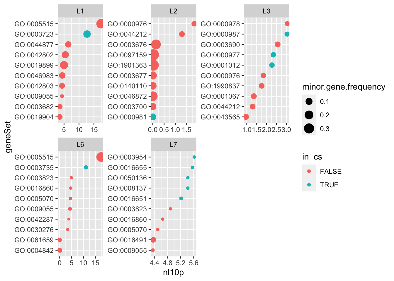
| Version | Author | Date |
|---|---|---|
| 53ac4cb | karltayeb | 2022-04-07 |
do.or.plot(res.l10, x='loglik', s='minor.gene.frequency')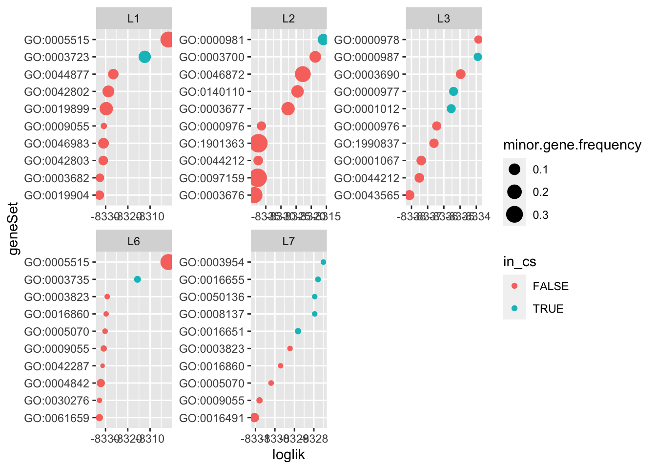
| Version | Author | Date |
|---|---|---|
| 53ac4cb | karltayeb | 2022-04-07 |
That could be because the multivariate regression is competing gene sets against eachother.
\(L=1\)
For the single effect regression (SER) \(L=1\) I would expect that ranking the effects by increasing PIP in the SER would give the same results as ranking the marginal univariate regressions by increasing likelihood. But that’s not the case…
p1 <- do.or.plot(res.l1, x='nl10p', s='minor.gene.frequency')
p2 <-do.or.plot(res.l1, x='loglik', s='minor.gene.frequency')
cowplot::plot_grid(p1, p2, nrow = 1)
| Version | Author | Date |
|---|---|---|
| 53ac4cb | karltayeb | 2022-04-07 |
Two reasons this could be happening are (1) shrinkage of the effect sizes in the SER or (2) the SER estimates a shared intercept for all the gene sets.
So next we look at the SER but we fix the effect size variance to a large value so the prior is flat.
Flat prior on effect sizes
p1 <- do.or.plot(res.l1.flat, x='nl10p', s='minor.gene.frequency')
p2 <- do.or.plot(res.l1.flat, x='loglik', s='minor.gene.frequency')
cowplot::plot_grid(p1, p2, nrow = 1)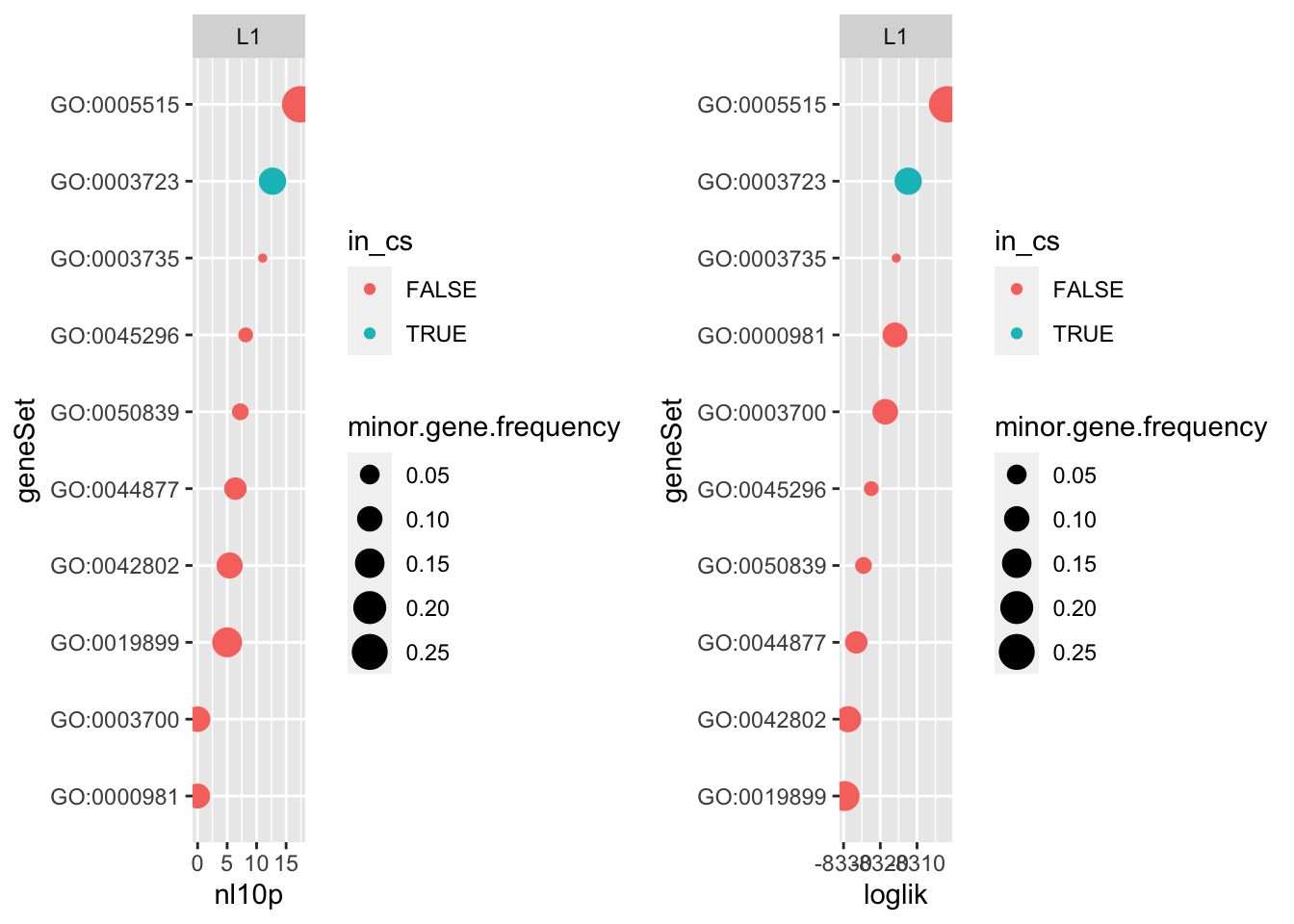
| Version | Author | Date |
|---|---|---|
| 53ac4cb | karltayeb | 2022-04-07 |
The results for “flat” SER are suspiciously similar to what we just showed. But if we look at mu for both fits they’re different. We see the expected shrinkage (although that’s a pretty funky shape– it looks like smaller gene sets experience stronger shrinkage which makes sense)
sizes <- colSums(genesets$gomf$X[, colnames(susie.l1$fit$mu)])
tbl <- tibble(
  flat.mu=susie.l1.flat$fit$mu[1,],
  mu=susie.l1$fit$mu[1,],
  size = sizes)

tbl %>%
  ggplot(aes(y=mu, x=flat.mu, color=log(size))) +
  geom_point()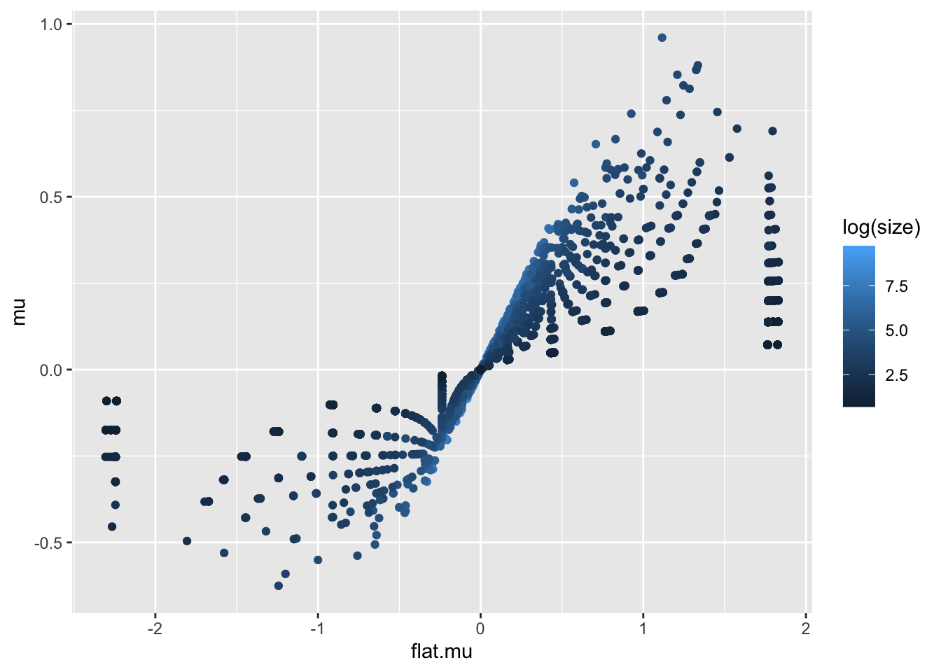
| Version | Author | Date |
|---|---|---|
| 53ac4cb | karltayeb | 2022-04-07 |
Fixed intercept in marginal regression
So could it be the intercept? I took the intercept estimated from SER and refit the univariate logistic regressions with a fixed intercept. For this example, it resolves the discrepancy.
marginal.fixed.intercept <-
  marginal.fixed.intercept %>%
  mutate(fixed.loglik = -(aic - 4)/2)

tmpa <-
  marginal_tbl %>%
  mutate(loglik = -(logistic.aic - 4)/2)

tmpb <- marginal.fixed.intercept %>%
  mutate(fixed.loglik = -(aic - 4)/2) %>%
  select(geneSet, fixed.loglik)

tmpc <- res.l1.flat
tmpc$geneset.summary <- tmpc$geneset.summary %>%
  left_join(tmpb)
Joining, by = "geneSet"tmpc$cs.summary <- tmpc$cs.summary %>%
left_join(tmpb)Joining, by = "geneSet"p1 <- do.or.plot(tmpc, x='loglik', s='minor.gene.frequency')
p2 <- do.or.plot(tmpc, x='fixed.loglik', s='minor.gene.frequency')
cowplot::plot_grid(p1, p2, nrow = 1)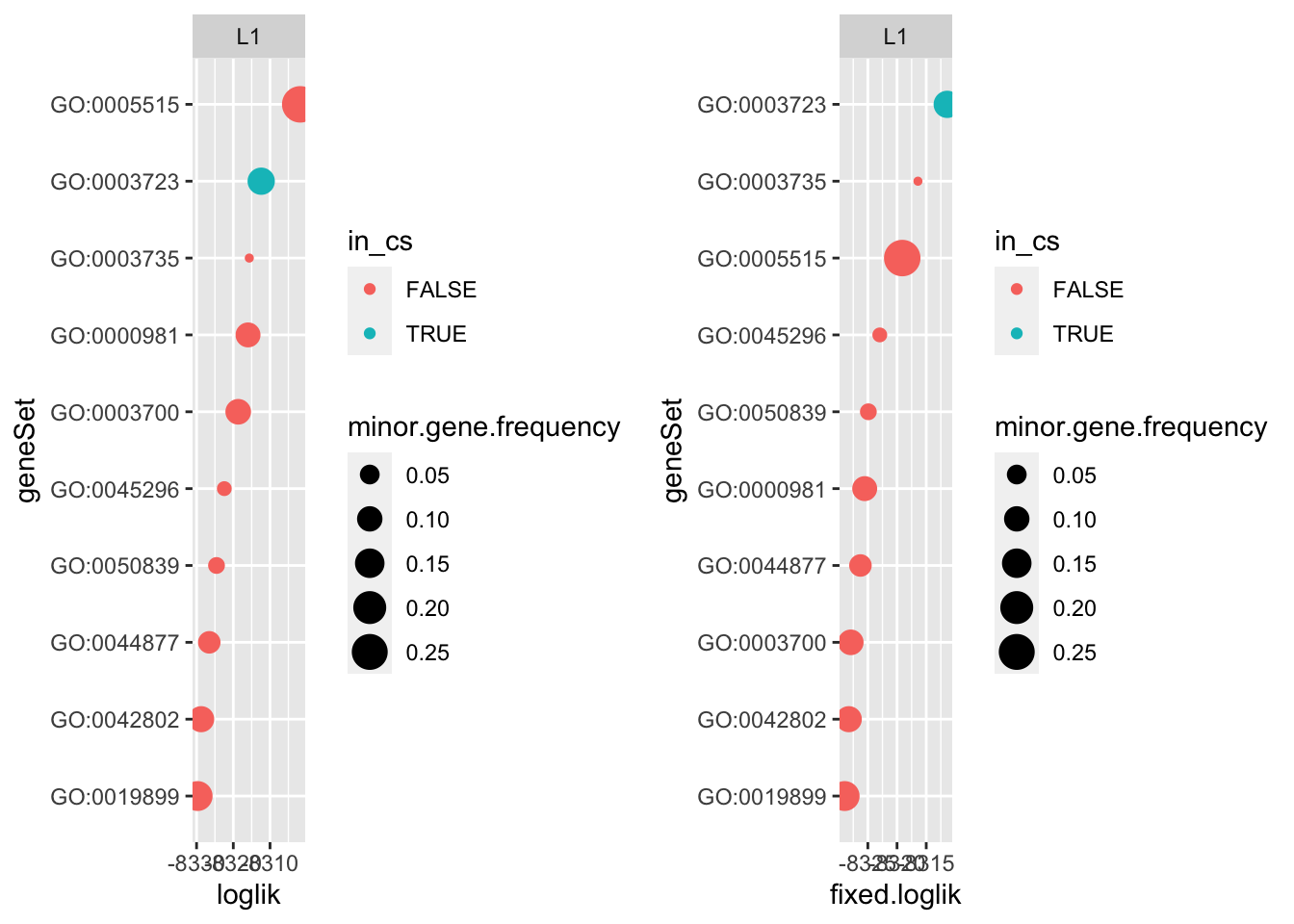
| Version | Author | Date |
|---|---|---|
| 53ac4cb | karltayeb | 2022-04-07 |
So once you fix the intercept the likelihoods track with the log(PIPs)…
p1 <- tmpc$geneset.summary %>%
  left_join(tmpb)%>%
  ggplot(aes(x=log(pip), y=loglik)) + geom_point()
Joining, by = c("geneSet", "fixed.loglik")p2 <- tmpc$geneset.summary %>%
left_join(tmpb)%>%
ggplot(aes(x=log(pip), y=fixed.loglik)) + geom_point()Joining, by = c("geneSet", "fixed.loglik")cowplot::plot_grid(p1, p2, nrow = 1)Warning: Removed 100 rows containing missing values (geom_point).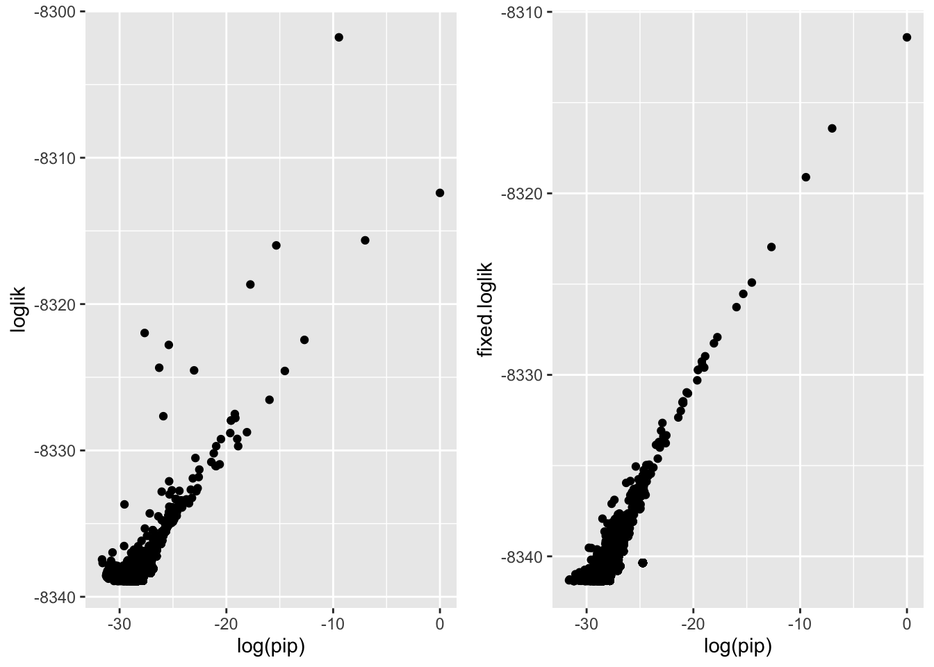
And here you can look at the likelihood of each univariate model with the fixed vs not fixed intercept…
tmpa %>%
  left_join(tmpb)%>%
  ggplot(aes(x=loglik, y=fixed.loglik)) + geom_point()
Joining, by = "geneSet"Warning: Removed 100 rows containing missing values (geom_point).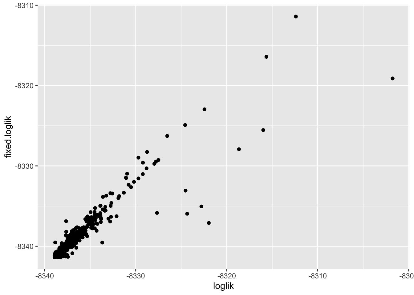
| Version | Author | Date |
|---|---|---|
| 53ac4cb | karltayeb | 2022-04-07 |
knitr::knit_exit()