Siblings analysis
2024-04-28
Last updated: 2024-06-26
Checks: 6 1
Knit directory: PODFRIDGE/
This reproducible R Markdown analysis was created with workflowr (version 1.7.1). The Checks tab describes the reproducibility checks that were applied when the results were created. The Past versions tab lists the development history.
Great! Since the R Markdown file has been committed to the Git repository, you know the exact version of the code that produced these results.
Great job! The global environment was empty. Objects defined in the global environment can affect the analysis in your R Markdown file in unknown ways. For reproduciblity it’s best to always run the code in an empty environment.
The command set.seed(20230302) was run prior to running
the code in the R Markdown file. Setting a seed ensures that any results
that rely on randomness, e.g. subsampling or permutations, are
reproducible.
Great job! Recording the operating system, R version, and package versions is critical for reproducibility.
Nice! There were no cached chunks for this analysis, so you can be confident that you successfully produced the results during this run.
Using absolute paths to the files within your workflowr project makes it difficult for you and others to run your code on a different machine. Change the absolute path(s) below to the suggested relative path(s) to make your code more reproducible.
| absolute | relative |
|---|---|
| /Users/linmatch/Documents/GitHub/PODFRIDGE | . |
Great! You are using Git for version control. Tracking code development and connecting the code version to the results is critical for reproducibility.
The results in this page were generated with repository version cdc3bd0. See the Past versions tab to see a history of the changes made to the R Markdown and HTML files.
Note that you need to be careful to ensure that all relevant files for
the analysis have been committed to Git prior to generating the results
(you can use wflow_publish or
wflow_git_commit). workflowr only checks the R Markdown
file, but you know if there are other scripts or data files that it
depends on. Below is the status of the Git repository when the results
were generated:
Ignored files:
    Ignored:    .DS_Store
    Ignored:    .Rhistory
    Ignored:    .Rproj.user/

Unstaged changes:
    Modified:   data/data_proportions.csv
Note that any generated files, e.g. HTML, png, CSS, etc., are not included in this status report because it is ok for generated content to have uncommitted changes.
These are the previous versions of the repository in which changes were
made to the R Markdown (analysis/siblings_analysis.Rmd) and
HTML (docs/siblings_analysis.html) files. If you’ve
configured a remote Git repository (see ?wflow_git_remote),
click on the hyperlinks in the table below to view the files as they
were in that past version.
| File | Version | Author | Date | Message |
|---|---|---|---|---|
| Rmd | cdc3bd0 | linmatch | 2024-06-26 | fer_dis |
| Rmd | 326ad11 | linmatch | 2024-06-26 | fert distribution |
| Rmd | 892720f | linmatch | 2024-06-23 | fert dis3 |
| Rmd | c865baa | linmatch | 2024-06-23 | fertility dis2 |
| Rmd | f2c131d | linmatch | 2024-06-23 | fertility distribution |
| html | bce5e2e | hcvw | 2024-05-27 | Build site. |
| Rmd | 332d5a2 | hcvw | 2024-05-27 | wflow_publish(c("analysis/CODIS_DB_composition.Rmd", "analysis/final_equation.Rmd", |
# load necessary libraryes
library(readr)
library(tidyverse)
library(tidyr)
library(ggplot2)
library(viridis)
library(dplyr)
library(knitr)

setwd("/Users/linmatch/Documents/GitHub/PODFRIDGE")

children_data = read.csv("./data/proportions_table_by_race_year.csv")
mother_data = read.csv("./data/data_filtered_recoded.csv")
ggplot(data = children_data,aes(x=chborn_num,y=proportion)) +
geom_col(position = position_dodge()) +
facet_grid(RACE~YEAR) + theme_classic()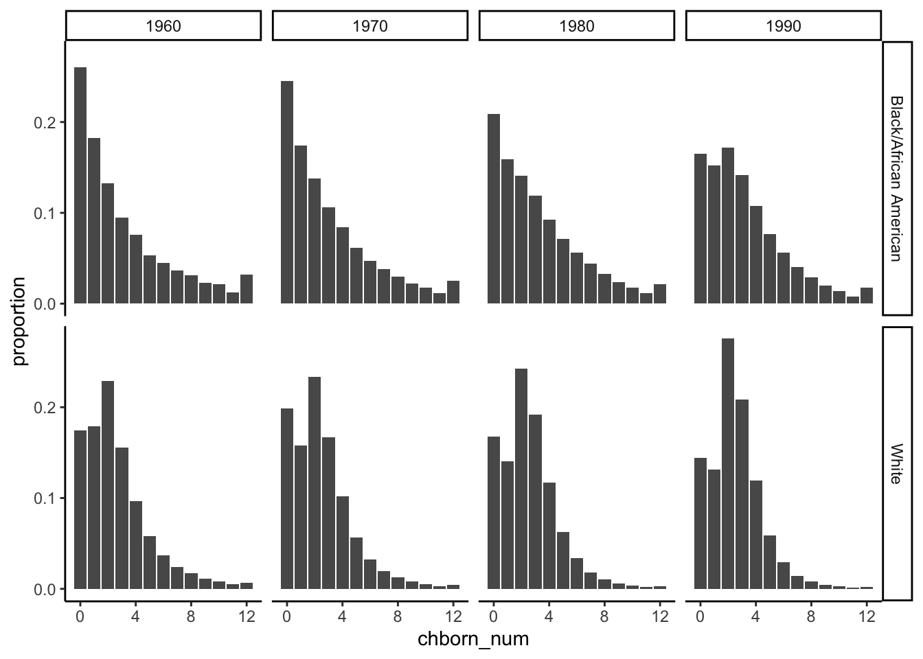
| Version | Author | Date |
|---|---|---|
| bce5e2e | hcvw | 2024-05-27 |
mother_data <- mother_data %>% mutate(id = row_number())
child_df = as.data.frame(rep(mother_data$id,mother_data$chborn_num))
colnames(child_df) = "id"
child_df = merge(child_df,mother_data,by="id")
child_df$nsib = child_df$chborn_num - 1

child_df_gb = child_df %>%
  group_by(RACE,nsib) %>%
  summarise(count = n())
`summarise()` has grouped output by 'RACE'. You can override using the
`.groups` argument.child_df_gb$prob = ifelse(child_df_gb$RACE == "White",child_df_gb$count/4380009, child_df_gb$count/547692)
ggplot(data = child_df_gb, aes(x = nsib, y = prob)) +
geom_col(position = position_dodge()) +
facet_wrap(~RACE) + theme_classic()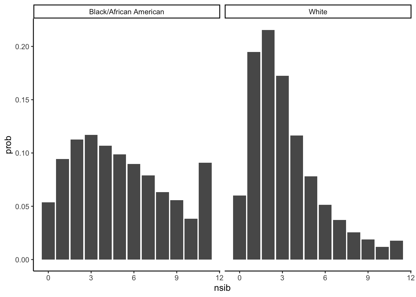
| Version | Author | Date |
|---|---|---|
| bce5e2e | hcvw | 2024-05-27 |
Probability of a person of each race having each number of siblings
colnames(child_df_gb) = c("Race","Number of Siblings","Count",'Probability')
kable(child_df_gb[,c(1,2,4)])| Race | Number of Siblings | Probability |
|---|---|---|
| Black/African American | 0 | 0.0536835 |
| Black/African American | 1 | 0.0944034 |
| Black/African American | 2 | 0.1126400 |
| Black/African American | 3 | 0.1169489 |
| Black/African American | 4 | 0.1069123 |
| Black/African American | 5 | 0.0987928 |
| Black/African American | 6 | 0.0895686 |
| Black/African American | 7 | 0.0788034 |
| Black/African American | 8 | 0.0633805 |
| Black/African American | 9 | 0.0556882 |
| Black/African American | 10 | 0.0383610 |
| Black/African American | 11 | 0.0908175 |
| White | 0 | 0.0599540 |
| White | 1 | 0.1948590 |
| White | 2 | 0.2154482 |
| White | 3 | 0.1725750 |
| White | 4 | 0.1163034 |
| White | 5 | 0.0780464 |
| White | 6 | 0.0513892 |
| White | 7 | 0.0372693 |
| White | 8 | 0.0256068 |
| White | 9 | 0.0188150 |
| White | 10 | 0.0119091 |
| White | 11 | 0.0178246 |
Here, we are trying to create a frequency table to show the number of children born, the number of mother who has “chborn_num” children, the number of sibling, and the number of individuals who has “n_sib” siblings. - n_sib = chborn_num - 1 - freq_n_sib = freq_mother * chborn_num eg.Suppose 10 mothers (generation 0) has 7 children, then there will be 70 children (generation 1) in total who has 6 siblings.
blue_colors <- c("#0000FF", "#0000E5", "#0000CC", "#0000B2", "#000099", "#00007F", "#000066",
                 "#00004C", "#000033", "#000019", "#3333FF", "#6666FF", "#9999FF")

unique_chborn_num <- sort(unique(mother_data$chborn_num))
color_mapping <- setNames(blue_colors, unique_chborn_num)
fert_df <- mother_data %>%
count(RACE, YEAR, chborn_num) %>%
arrange(RACE, YEAR, chborn_num) %>%
mutate(n_sib = chborn_num -1, freq_n_sib = n * chborn_num,
color = color_mapping[as.character(chborn_num)]) %>%
rename(freq_mother = n)
print(fert_df) RACE YEAR chborn_num freq_mother n_sib freq_n_sib color
1 Black/African American 1960 0 6697 -1 0 #0000FF
2 Black/African American 1960 1 4698 0 4698 #0000E5
3 Black/African American 1960 2 3411 1 6822 #0000CC
4 Black/African American 1960 3 2445 2 7335 #0000B2
5 Black/African American 1960 4 1949 3 7796 #000099
6 Black/African American 1960 5 1361 4 6805 #00007F
7 Black/African American 1960 6 1162 5 6972 #000066
8 Black/African American 1960 7 932 6 6524 #00004C
9 Black/African American 1960 8 810 7 6480 #000033
10 Black/African American 1960 9 588 8 5292 #000019
11 Black/African American 1960 10 549 9 5490 #3333FF
12 Black/African American 1960 11 326 10 3586 #6666FF
13 Black/African American 1960 12 821 11 9852 #9999FF
14 Black/African American 1970 0 16490 -1 0 #0000FF
15 Black/African American 1970 1 11686 0 11686 #0000E5
16 Black/African American 1970 2 9275 1 18550 #0000CC
17 Black/African American 1970 3 7161 2 21483 #0000B2
18 Black/African American 1970 4 5659 3 22636 #000099
19 Black/African American 1970 5 4147 4 20735 #00007F
20 Black/African American 1970 6 3147 5 18882 #000066
21 Black/African American 1970 7 2542 6 17794 #00004C
22 Black/African American 1970 8 2012 7 16096 #000033
23 Black/African American 1970 9 1473 8 13257 #000019
24 Black/African American 1970 10 1194 9 11940 #3333FF
25 Black/African American 1970 11 784 10 8624 #6666FF
26 Black/African American 1970 12 1682 11 20184 #9999FF
27 Black/African American 1980 0 8417 -1 0 #0000FF
28 Black/African American 1980 1 6383 0 6383 #0000E5
29 Black/African American 1980 2 5681 1 11362 #0000CC
30 Black/African American 1980 3 4797 2 14391 #0000B2
31 Black/African American 1980 4 3732 3 14928 #000099
32 Black/African American 1980 5 2870 4 14350 #00007F
33 Black/African American 1980 6 2264 5 13584 #000066
34 Black/African American 1980 7 1782 6 12474 #00004C
35 Black/African American 1980 8 1310 7 10480 #000033
36 Black/African American 1980 9 943 8 8487 #000019
37 Black/African American 1980 10 717 9 7170 #3333FF
38 Black/African American 1980 11 452 10 4972 #6666FF
39 Black/African American 1980 12 870 11 10440 #9999FF
40 Black/African American 1990 0 7193 -1 0 #0000FF
41 Black/African American 1990 1 6635 0 6635 #0000E5
42 Black/African American 1990 2 7485 1 14970 #0000CC
43 Black/African American 1990 3 6161 2 18483 #0000B2
44 Black/African American 1990 4 4673 3 18692 #000099
45 Black/African American 1990 5 3333 4 16665 #00007F
46 Black/African American 1990 6 2445 5 14670 #000066
47 Black/African American 1990 7 1752 6 12264 #00004C
48 Black/African American 1990 8 1263 7 10104 #000033
49 Black/African American 1990 9 853 8 7677 #000019
50 Black/African American 1990 10 590 9 5900 #3333FF
51 Black/African American 1990 11 348 10 3828 #6666FF
52 Black/African American 1990 12 772 11 9264 #9999FF
53 White 1960 0 46202 -1 0 #0000FF
54 White 1960 1 47433 0 47433 #0000E5
55 White 1960 2 60732 1 121464 #0000CC
56 White 1960 3 41272 2 123816 #0000B2
57 White 1960 4 25666 3 102664 #000099
58 White 1960 5 15327 4 76635 #00007F
59 White 1960 6 9697 5 58182 #000066
60 White 1960 7 6347 6 44429 #00004C
61 White 1960 8 4518 7 36144 #000033
62 White 1960 9 2990 8 26910 #000019
63 White 1960 10 2148 9 21480 #3333FF
64 White 1960 11 1280 10 14080 #6666FF
65 White 1960 12 1747 11 20964 #9999FF
66 White 1970 0 133940 -1 0 #0000FF
67 White 1970 1 106663 0 106663 #0000E5
68 White 1970 2 157405 1 314810 #0000CC
69 White 1970 3 112397 2 337191 #0000B2
70 White 1970 4 68603 3 274412 #000099
71 White 1970 5 38000 4 190000 #00007F
72 White 1970 6 22023 5 132138 #000066
73 White 1970 7 12927 6 90489 #00004C
74 White 1970 8 8534 7 68272 #000033
75 White 1970 9 5342 8 48078 #000019
76 White 1970 10 3593 9 35930 #3333FF
77 White 1970 11 2082 10 22902 #6666FF
78 White 1970 12 2858 11 34296 #9999FF
79 White 1980 0 61909 -1 0 #0000FF
80 White 1980 1 51856 0 51856 #0000E5
81 White 1980 2 89551 1 179102 #0000CC
82 White 1980 3 70716 2 212148 #0000B2
83 White 1980 4 43190 3 172760 #000099
84 White 1980 5 23170 4 115850 #00007F
85 White 1980 6 12556 5 75336 #000066
86 White 1980 7 6589 6 46123 #00004C
87 White 1980 8 3874 7 30992 #000033
88 White 1980 9 2254 8 20286 #000019
89 White 1980 10 1368 9 13680 #3333FF
90 White 1980 11 757 10 8327 #6666FF
91 White 1980 12 1073 11 12876 #9999FF
92 White 1990 0 62471 -1 0 #0000FF
93 White 1990 1 56647 0 56647 #0000E5
94 White 1990 2 119054 1 238108 #0000CC
95 White 1990 3 90170 2 270510 #0000B2
96 White 1990 4 51511 3 206044 #000099
97 White 1990 5 25385 4 126925 #00007F
98 White 1990 6 12698 5 76188 #000066
99 White 1990 7 6292 6 44044 #00004C
100 White 1990 8 3479 7 27832 #000033
101 White 1990 9 1876 8 16884 #000019
102 White 1990 10 1132 9 11320 #3333FF
103 White 1990 11 623 10 6853 #6666FF
104 White 1990 12 828 11 9936 #9999FFfert_df_black <- fert_df %>% filter(RACE == "Black/African American")
fert_df_white <- fert_df %>% filter(RACE == "White")
df_long1 <- fert_df_black %>%
pivot_longer(cols = c(freq_mother, freq_n_sib),
names_to = "frequency_type",
values_to = "frequency") %>%
mutate(x_axis = ifelse(frequency_type == "freq_mother", chborn_num, n_sib))ggplot(df_long1, aes(x = x_axis, y = frequency, fill = as.factor(x_axis))) +
geom_col() +
facet_grid(frequency_type ~ YEAR, scales = "free",
labeller = labeller(frequency_type = c("freq_mother" = "Number of Children Born",
"freq_n_sib" = "Number of Siblings"),
YEAR = function(x) paste("Year", x))) +
scale_fill_viridis_d(option = "plasma", name = "Number of Children/Siblings") +
labs(title = "Distribution of Number of Children/Siblings by Census Year",
x = "Number of Children/Siblings",
y = "Frequency") +
theme_minimal() +
theme(axis.text.x = element_text(angle = 45, hjust = 1),
legend.position = "right")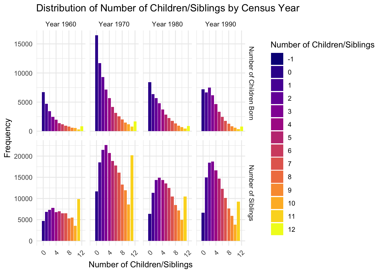
sessionInfo()R version 4.3.2 (2023-10-31)
Platform: x86_64-apple-darwin20 (64-bit)
Running under: macOS Monterey 12.7.4
Matrix products: default
BLAS: /Library/Frameworks/R.framework/Versions/4.3-x86_64/Resources/lib/libRblas.0.dylib
LAPACK: /Library/Frameworks/R.framework/Versions/4.3-x86_64/Resources/lib/libRlapack.dylib; LAPACK version 3.11.0
locale:
[1] en_US.UTF-8/en_US.UTF-8/en_US.UTF-8/C/en_US.UTF-8/en_US.UTF-8
time zone: America/New_York
tzcode source: internal
attached base packages:
[1] stats graphics grDevices utils datasets methods base
other attached packages:
[1] knitr_1.45 viridis_0.6.5 viridisLite_0.4.2 lubridate_1.9.3
[5] forcats_1.0.0 stringr_1.5.1 dplyr_1.1.4 purrr_1.0.2
[9] tidyr_1.3.1 tibble_3.2.1 ggplot2_3.4.4 tidyverse_2.0.0
[13] readr_2.1.5 workflowr_1.7.1
loaded via a namespace (and not attached):
[1] sass_0.4.8 utf8_1.2.4 generics_0.1.3 stringi_1.8.3
[5] hms_1.1.3 digest_0.6.34 magrittr_2.0.3 timechange_0.3.0
[9] evaluate_0.23 grid_4.3.2 fastmap_1.1.1 rprojroot_2.0.4
[13] jsonlite_1.8.8 processx_3.8.3 whisker_0.4.1 gridExtra_2.3
[17] ps_1.7.6 promises_1.2.1 httr_1.4.7 fansi_1.0.6
[21] scales_1.3.0 jquerylib_0.1.4 cli_3.6.2 rlang_1.1.3
[25] munsell_0.5.0 withr_3.0.0 cachem_1.0.8 yaml_2.3.8
[29] tools_4.3.2 tzdb_0.4.0 colorspace_2.1-0 httpuv_1.6.14
[33] vctrs_0.6.5 R6_2.5.1 lifecycle_1.0.4 git2r_0.33.0
[37] fs_1.6.3 pkgconfig_2.0.3 callr_3.7.3 pillar_1.9.0
[41] bslib_0.6.1 later_1.3.2 gtable_0.3.4 glue_1.7.0
[45] Rcpp_1.0.12 xfun_0.41 tidyselect_1.2.1 highr_0.10
[49] rstudioapi_0.15.0 farver_2.1.1 htmltools_0.5.7 labeling_0.4.3
[53] rmarkdown_2.25 compiler_4.3.2 getPass_0.2-4