Regression to predict CODIS database proportions
2024-04-28
Last updated: 2024-06-25
Checks: 7 0
Knit directory: PODFRIDGE/
This reproducible R Markdown analysis was created with workflowr (version 1.7.1). The Checks tab describes the reproducibility checks that were applied when the results were created. The Past versions tab lists the development history.
Great! Since the R Markdown file has been committed to the Git repository, you know the exact version of the code that produced these results.
Great job! The global environment was empty. Objects defined in the global environment can affect the analysis in your R Markdown file in unknown ways. For reproduciblity it’s best to always run the code in an empty environment.
The command set.seed(20230302) was run prior to running the code in the R Markdown file. Setting a seed ensures that any results that rely on randomness, e.g. subsampling or permutations, are reproducible.
Great job! Recording the operating system, R version, and package versions is critical for reproducibility.
Nice! There were no cached chunks for this analysis, so you can be confident that you successfully produced the results during this run.
Great job! Using relative paths to the files within your workflowr project makes it easier to run your code on other machines.
Great! You are using Git for version control. Tracking code development and connecting the code version to the results is critical for reproducibility.
The results in this page were generated with repository version 1eb6d2c. See the Past versions tab to see a history of the changes made to the R Markdown and HTML files.
Note that you need to be careful to ensure that all relevant files for the analysis have been committed to Git prior to generating the results (you can use wflow_publish or wflow_git_commit). workflowr only checks the R Markdown file, but you know if there are other scripts or data files that it depends on. Below is the status of the Git repository when the results were generated:
Untracked files:
    Untracked:  PODFRIDGE/
    Untracked:  Rplots.pdf

Unstaged changes:
    Modified:   analysis/final_equation.Rmd
Note that any generated files, e.g. HTML, png, CSS, etc., are not included in this status report because it is ok for generated content to have uncommitted changes.
These are the previous versions of the repository in which changes were made to the R Markdown (analysis/regression.Rmd) and HTML (docs/regression.html) files. If you’ve configured a remote Git repository (see ?wflow_git_remote), click on the hyperlinks in the table below to view the files as they were in that past version.
| File | Version | Author | Date | Message |
|---|---|---|---|---|
| html | 1eb6d2c | hcvw | 2024-06-25 | Build site. |
| Rmd | 96b197a | hcvw | 2024-06-25 | wflow_publish(c(“analysis/regression.Rmd”)) |
# Load necessary libraries
library(readr)
library(tidycensus)
library(tidyverse)
library(knitr)
library(jtools)
library(sandwich)

# Load prison data
prison_data = read.csv("./data/populations_states.csv")

# Load CODIS data
codis_data = read.csv("./data/CODIS_data.csv")

# Create a data frame for Murphy and Tong profiles
murphy.tong = data.frame(
  state = c("California", "Florida", "Indiana", "Maine", "Nevada", "South Dakota", "Texas"),
  total = c(2768269, 1350667, 307714, 32847, 167726, 67600, 960985,2768269, 1350667, 307714, 32847, 167726, 67600, 960985),
  mt.percent = c(0.296, 0.614, 0.7, 0.928, 0.694, 0.668, 0.373,0.171, 0.352, 0.26, 0.039, 0.256, 0.06, 0.291),
  race = c("White","White","White","White","White","White","White","Black","Black","Black","Black","Black","Black","Black")
)
# Load necessary libraries
# Calculate the number of White and Black profiles in Murphy and Tong data
murphy.tong$n = murphy.tong$total * murphy.tong$mt.percent
# Extract year from the date and filter data for 2022
prison_data$year = substring(prison_data$date, 1, 4)
prison_data_2022 = prison_data[which(prison_data$year == "2022"),]
prison_data_2022 = prison_data_2022[!duplicated(prison_data_2022[, 'state']),]
# Load census data for each state
# P1_002N is the total population, P1_003N is the total White population, and P1_004N is the total Black population
us_state_density <- get_decennial(
geography = "state",
variables = c(all = "P1_002N", white = "P1_003N", black = "P1_004N"),
year = 2020,
geometry = TRUE,
keep_geo_vars = TRUE
)
# Spread the data into a wider format
us_state_density = spread(us_state_density, variable, value)
# Calculate the proportion of Black and White populations
us_state_density$census.percent.black = us_state_density$black / us_state_density$all
us_state_density$census.percent.white = us_state_density$white / us_state_density$all
# Rename column for merging
us_state_density$state = us_state_density$NAME.x
# Merge census data with prison data
us_state_density = merge(us_state_density, prison_data_2022, by = "state")
# Calculate the proportion of Black and White incarcerated individuals
us_state_density$percent.black.incarc = us_state_density$incarcerated_black / us_state_density$incarcerated_total
us_state_density$percent.white.incarc = us_state_density$incarcerated_white / us_state_density$incarcerated_total
# Merge with CODIS data
us_state_density = merge(us_state_density, codis_data, by = "state")
# Calculate the number of Black and White profiles in CODIS
us_state_density$black_profiles = us_state_density$percent.black.incarc * (us_state_density$offender_profiles)
us_state_density$white_profiles = us_state_density$percent.white.incarc * (us_state_density$offender_profiles)
us_state_density_black = as.data.frame(us_state_density[,c("state","all","black","census.percent.black","incarcerated_total",
"incarcerated_black","percent.black.incarc","arrestee_profiles","offender_profiles","black_profiles")])
us_state_density_black$race = "Black"
colnames(us_state_density_black) = c("state","all","population","census.percent","incarcerated_total",
"incarcerated_race","percent.incar","arrestee_profiles","offender_profiles","geometry","race_profiles","race")
us_state_density_white = as.data.frame(us_state_density[,c("state","all","white","census.percent.white","incarcerated_total",
"incarcerated_white","percent.white.incarc", "arrestee_profiles","offender_profiles","white_profiles")])
us_state_density_white$race = "White"
colnames(us_state_density_white) = c("state","all","population","census.percent","incarcerated_total",
"incarcerated_race","percent.incar","arrestee_profiles","offender_profiles","geometry","race_profiles","race")
inferred_data = rbind(us_state_density_black, us_state_density_white)
# Combine Murphy and Tong data with the merged dataset
combined = merge(murphy.tong, inferred_data, by = c("state","race"), all.x = TRUE)
combined$race_bin = ifelse(combined$race == "White",0,1)# Fit linear models for Black and White population proportions
model.all <- lm(
mt.percent ~ # Outcome: Murphy & Tong numbers for 7 states
census.percent + # Main effect of census proportion on CODIS proportion
percent.incar + # Main effect of prison proportion on CODIS proportion
race_bin+ # Main effect of race. This will estimate the change in CODIS proportion for different races relative to a baseline race.
race_bin:census.percent + # Interaction between race and census proportion.
# This checks if the effect of census proportion on CODIS proportion varies by race.
race_bin:percent.incar, # Interaction between race and prison proportion.
# This checks if the effect of prison proportion on CODIS proportion varies by race.
data = combined # The data set containing the variables
)
summary(model.all)
plot_summs(model.all, robust = TRUE)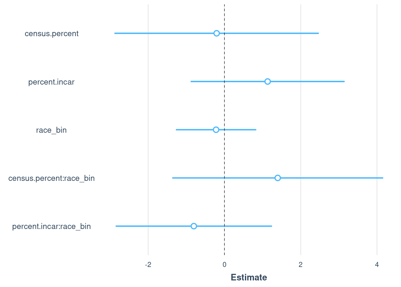
| Version | Author | Date |
|---|---|---|
| 1eb6d2c | hcvw | 2024-06-25 |
# Run regression model for different combinations of the following predictors:
# race, census proportion of race, estimated population from Klein data
formula_a = "census.percent + percent.incar + race_bin" # no interactions
formula_b = "percent.incar + race_bin + race_bin:percent.incar" # no census
formula_c = "percent.incar + race_bin"  # no census or interaction
formula_d = "census.percent + percent.incar" # no race

formulas = c(formula_a, formula_b, formula_c, formula_d)

model_df = as.data.frame(matrix(0,nrow = 4, ncol = 3))
colnames(model_df) = c("model","R^2","Anova")
for(i in 1:4){
  form = formulas[[i]]
  model <- lm(paste0('mt.percent ~', form), data = combined)
  p.val = round(anova(model, model.all)[[6]][2],2)
  model_df[i,] = c(form, round(summary(model)$adj.r.squared,2),p.val)
}
kable(model_df)

# generate predictions based on the model with all coefficients
combined$prediction = predict(model.all, combined)
# Plot the results with linear regression lines
ggplot(data = combined) +
geom_point(aes(x = prediction, y = mt.percent,fill=state,shape = race),size=5,col="black") +
scale_shape_manual(name="Race",labels = c("Black","White"),values = c(21,24)) +
geom_abline(intercept = 0, slope = 1,col ="grey30", linetype = "dashed",size=1.5) +
theme_classic() + xlab("Estimated CODIS profiles") + ylab("Murphy & Tong profiles (FOIA)") +
annotate("text", x=0.2, y=0.75, size = 6, label= paste0(as.expression("R² = "), round(summary(model)$adj.r.squared,2))) +
annotate("text", x=0.6, y=0.56, size = 4, label= "Perfect prediction line",angle = 46) +
guides(fill=guide_legend(override.aes=list(shape=21))) +
theme(axis.text.x = element_text(color = "black", size = 16, angle = 0, hjust = .5, vjust = .5, face = "plain"),
axis.text.y = element_text(color = "black", size = 16, angle = 0, hjust = 1, vjust = 0, face = "plain"),
axis.title.x = element_text(color = "black", size = 16, angle = 0, hjust = .5, vjust = 0, face = "plain"),
axis.title.y = element_text(color = "black", size = 16, angle = 90, hjust = .5, vjust = .5, face = "plain"),
aspect.ratio=1) 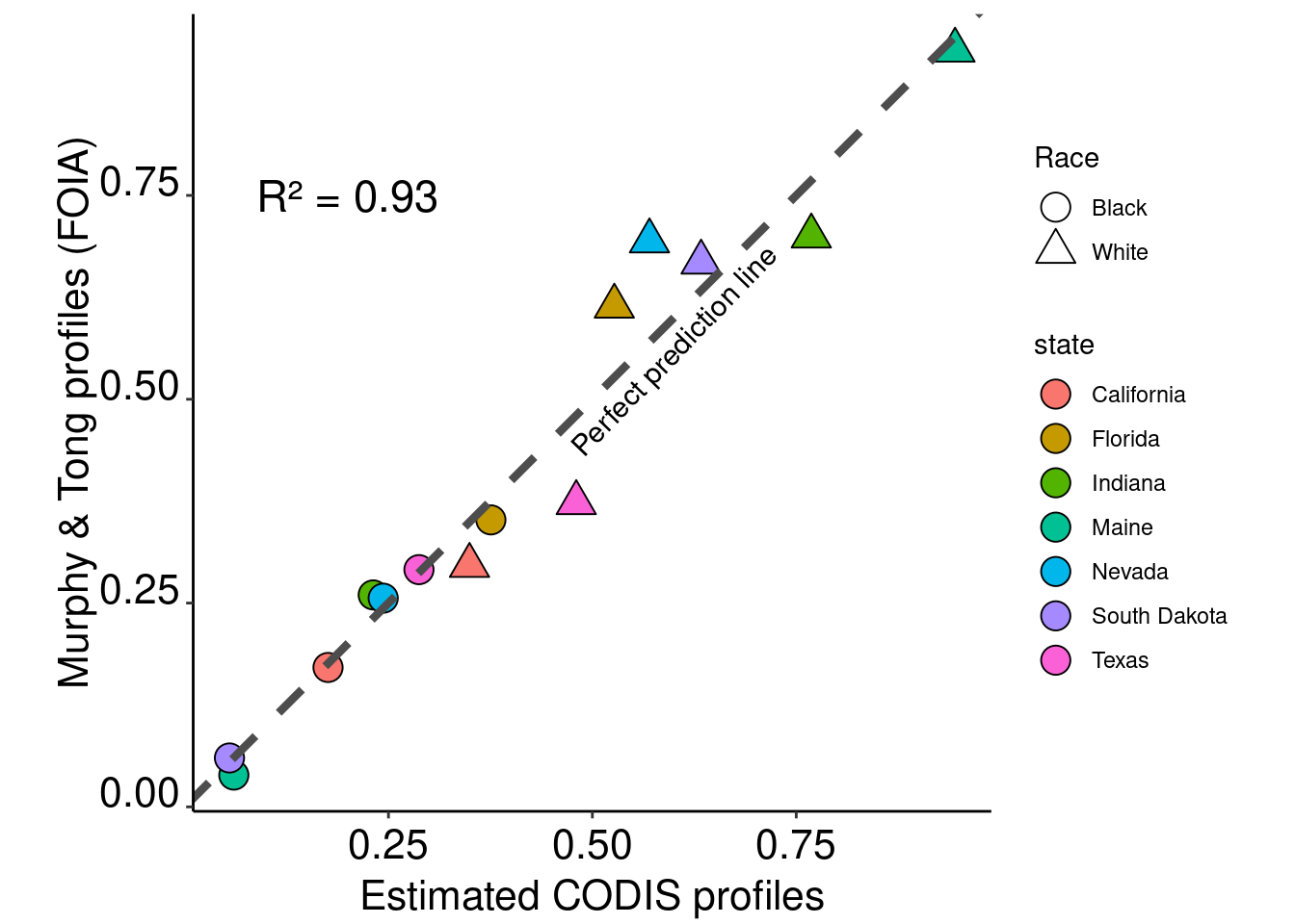
| Version | Author | Date |
|---|---|---|
| 1eb6d2c | hcvw | 2024-06-25 |
combined$Dif <- combined$prediction - combined$mt.percent
combined$Avg <- (combined$prediction + combined$mt.percent) / 2

ggplot(combined, aes(x = Avg, y = Dif)) +
  geom_point(aes(shape = race,fill=state),size=4,col="black") +
  scale_fill_discrete(name = "State") +
  guides(fill=guide_legend(override.aes=list(shape=21))) +
  scale_shape_manual(name="Race",labels = c("Black","White"),values = c(21,24)) +
  geom_hline(yintercept = mean(combined$Dif), colour = "black", size = 1) +
  geom_hline(yintercept = mean(combined$Dif) - (1.96 * sd(combined$Dif)), colour = "grey30", size = 0.5) +
  geom_hline(yintercept = mean(combined$Dif) + (1.96 * sd(combined$Dif)), colour = "grey30", size = 0.5) +
  ylab("Difference Between Measures") +
  xlab("Average Measure") + theme_light() +
  theme(axis.text.x = element_text(color = "black", size = 16, angle = 0, hjust = .5, vjust = .5, face = "plain"),
        axis.text.y = element_text(color = "black", size = 16, angle = 0, hjust = 1, vjust = 0, face = "plain"),
        axis.title.x = element_text(color = "black", size = 16, angle = 0, hjust = .5, vjust = 0, face = "plain"),
        axis.title.y = element_text(color = "black", size = 16, angle = 90, hjust = .5, vjust = .5, face = "plain"),
aspect.ratio=1) 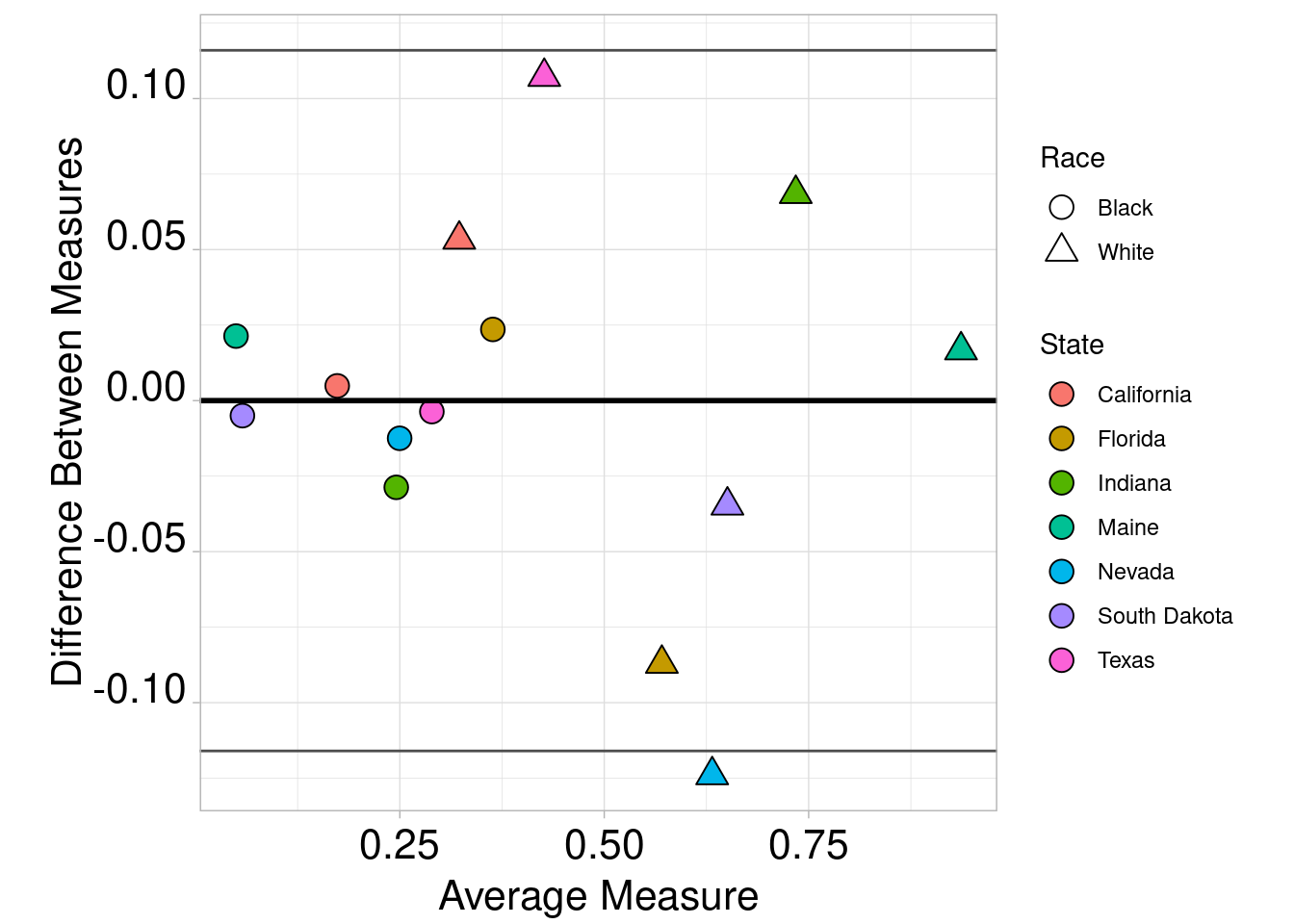
| Version | Author | Date |
|---|---|---|
| 1eb6d2c | hcvw | 2024-06-25 |
sessionInfo()R version 4.3.1 (2023-06-16)
Platform: x86_64-pc-linux-gnu (64-bit)
Running under: Ubuntu 22.04.3 LTS
Matrix products: default
BLAS: /usr/lib/x86_64-linux-gnu/openblas-pthread/libblas.so.3
LAPACK: /usr/lib/x86_64-linux-gnu/openblas-pthread/libopenblasp-r0.3.20.so; LAPACK version 3.10.0
locale:
[1] LC_CTYPE=en_US.UTF-8 LC_NUMERIC=C
[3] LC_TIME=en_US.UTF-8 LC_COLLATE=en_US.UTF-8
[5] LC_MONETARY=en_US.UTF-8 LC_MESSAGES=en_US.UTF-8
[7] LC_PAPER=en_US.UTF-8 LC_NAME=C
[9] LC_ADDRESS=C LC_TELEPHONE=C
[11] LC_MEASUREMENT=en_US.UTF-8 LC_IDENTIFICATION=C
time zone: America/New_York
tzcode source: system (glibc)
attached base packages:
[1] stats graphics grDevices utils datasets methods base
other attached packages:
[1] sandwich_3.1-0 jtools_2.2.2 knitr_1.46 lubridate_1.9.3
[5] forcats_1.0.0 stringr_1.5.0 dplyr_1.1.4 purrr_1.0.2
[9] tidyr_1.3.0 tibble_3.2.1 ggplot2_3.5.0 tidyverse_2.0.0
[13] tidycensus_1.4.4 readr_2.1.4 workflowr_1.7.1
loaded via a namespace (and not attached):
[1] gtable_0.3.3 xfun_0.44 bslib_0.5.1 tigris_2.0.3
[5] processx_3.8.4 lattice_0.21-8 callr_3.7.3 tzdb_0.4.0
[9] vctrs_0.6.5 tools_4.3.1 ps_1.7.6 generics_0.1.3
[13] curl_5.0.2 proxy_0.4-27 fansi_1.0.6 highr_0.10
[17] pkgconfig_2.0.3 KernSmooth_2.23-22 uuid_1.1-1 lifecycle_1.0.4
[21] farver_2.1.1 compiler_4.3.1 git2r_0.33.0 munsell_0.5.0
[25] getPass_0.2-4 httpuv_1.6.11 htmltools_0.5.6 class_7.3-22
[29] sass_0.4.7 yaml_2.3.7 later_1.3.1 pillar_1.9.0
[33] crayon_1.5.2 jquerylib_0.1.4 whisker_0.4.1 ellipsis_0.3.2
[37] classInt_0.4-9 cachem_1.0.8 tidyselect_1.2.0 rvest_1.0.3
[41] digest_0.6.33 stringi_1.7.12 pander_0.6.5 sf_1.0-14
[45] labeling_0.4.2 rprojroot_2.0.3 fastmap_1.1.1 grid_4.3.1
[49] colorspace_2.1-0 cli_3.6.2 magrittr_2.0.3 utf8_1.2.4
[53] broom_1.0.5 e1071_1.7-13 withr_3.0.0 backports_1.4.1
[57] scales_1.3.0 promises_1.2.1 rappdirs_0.3.3 timechange_0.2.0
[61] rmarkdown_2.25 httr_1.4.7 zoo_1.8-12 hms_1.1.3
[65] evaluate_0.21 rlang_1.1.3 Rcpp_1.0.11 glue_1.7.0
[69] DBI_1.1.3 xml2_1.3.5 rstudioapi_0.15.0 jsonlite_1.8.8
[73] R6_2.5.1 fs_1.6.3 units_0.8-3