Last updated: 2025-04-10

Checks: 6 1

Knit directory: QUAIL-Mex/

This reproducible R Markdown analysis was created with workflowr (version 1.7.1). The Checks tab describes the reproducibility checks that were applied when the results were created. The Past versions tab lists the development history.

R Markdown file: uncommitted changes

The R Markdown file has unstaged changes. To know which version of the R Markdown file created these results, you’ll want to first commit it to the Git repo. If you’re still working on the analysis, you can ignore this warning. When you’re finished, you can run wflow_publish to commit the R Markdown file and build the HTML.

Environment: empty

Great job! The global environment was empty. Objects defined in the global environment can affect the analysis in your R Markdown file in unknown ways. For reproduciblity it’s best to always run the code in an empty environment.

Seed: set.seed(20241009)

The command set.seed(20241009) was run prior to running the code in the R Markdown file. Setting a seed ensures that any results that rely on randomness, e.g. subsampling or permutations, are reproducible.

Session information: recorded

Great job! Recording the operating system, R version, and package versions is critical for reproducibility.

Cache: none

Nice! There were no cached chunks for this analysis, so you can be confident that you successfully produced the results during this run.

File paths: relative

Great job! Using relative paths to the files within your workflowr project makes it easier to run your code on other machines.

Repository version: 3ca4968

Great! You are using Git for version control. Tracking code development and connecting the code version to the results is critical for reproducibility.

The results in this page were generated with repository version 3ca4968. See the Past versions tab to see a history of the changes made to the R Markdown and HTML files.

Note that you need to be careful to ensure that all relevant files for the analysis have been committed to Git prior to generating the results (you can use wflow_publish or wflow_git_commit). workflowr only checks the R Markdown file, but you know if there are other scripts or data files that it depends on. Below is the status of the Git repository when the results were generated:


Ignored files:
    Ignored:    .DS_Store
    Ignored:    .RData
    Ignored:    .Rhistory
    Ignored:    .Rproj.user/
    Ignored:    analysis/.DS_Store
    Ignored:    analysis/.RData
    Ignored:    analysis/.Rhistory
    Ignored:    analysis/HLTH_counts_by_SES.png
    Ignored:    analysis/Hrs_by_HWISE score.png
    Ignored:    analysis/odds_ratio_plot.png
    Ignored:    analysis/stacked_barplot.png
    Ignored:    code/.DS_Store
    Ignored:    data/.DS_Store

Unstaged changes:
    Modified:   analysis/Plots_Latinx_research_week.Rmd

Note that any generated files, e.g. HTML, png, CSS, etc., are not included in this status report because it is ok for generated content to have uncommitted changes.

These are the previous versions of the repository in which changes were made to the R Markdown (analysis/Plots_Latinx_research_week.Rmd) and HTML (docs/Plots_Latinx_research_week.html) files. If you’ve configured a remote Git repository (see ?wflow_git_remote), click on the hyperlinks in the table below to view the files as they were in that past version.

File	Version	Author	Date	Message
Rmd	3ca4968	Paloma	2025-04-10	plots Sanaa
html	3ca4968	Paloma	2025-04-10	plots Sanaa
html	1453f8b	Paloma	2025-04-09	new urop plots
Rmd	c9896b1	Paloma	2025-02-25	ses-health
html	c9896b1	Paloma	2025-02-25	ses-health
Rmd	44474e3	Paloma	2025-02-22	Create Plots_Latinx_research_week.Rmd

Data cleaning

#Loading file and setting empty cells as "NAs"
d <- read.csv("./data/01.SCREENING.csv", stringsAsFactors = TRUE, na.strings = c("", " ","NA", "N/A"))


 # extract duplicates and compare values (removed manually for now)
dup <- d$ID[duplicated(d$ID)] 
length(dup) # 38

[1] 138

#print(dup)

# remove duplicates
d <- d[!duplicated(d$ID),]
# confirm total number of participants
length(unique(d$ID)) # 433 rows, but 394 participants

[1] 399

# What numbers are missing? 
ID <- as.ordered(d$ID)
# first trip
setdiff(1:204, ID)

[1]  71 164

nrow(d[d$ID <=250,])

[1] 202

# second trip
setdiff(301:497, ID)

integer(0)

nrow(d[d$ID >=250,])

[1] 197

nrow(d)

[1] 399

 #make ID number the row names
rownames(d) <- d$ID

# Code NAs
d[d=='NA'] <- NA
d <- d %>% 
    replace_na()

# Count rows with NAs
nrow(d[rowSums(is.na(d)) > 0,]) # 12 rows

[1] 399

nrow(d[!complete.cases(d),]) # 12 rows

[1] 399

#NAs <- d[rowSums(is.na(d))> 0,]
#write.table(NAs, "240301_SES_Age_NAs.csv", row.names=FALSE)

# Select useful information
d <- d %>% 
  select(ID, SES_EDU_SC, SES_BTHR_SC, SES_CAR_SC, SES_INT_SC, SES_WRK_SC, SES_BEDR_SC)

# transform factors to numbers
for (i in c(2:length(d))) {
    d[,i] <- as.numeric(as.character(d[,i]))
}

Warning: NAs introduced by coercion
Warning: NAs introduced by coercion

# Keep rows with no missing data
d <- d[complete.cases(d),] # - 9 (dup)  # total 382 complete cases, total 394
nrow(d)

[1] 349

head(d)

  ID SES_EDU_SC SES_BTHR_SC SES_CAR_SC SES_INT_SC SES_WRK_SC SES_BEDR_SC
1  1         10          24          0         31         61          23
2  2         31          47         18         31         46          23
3  3         31           0          0          0         15           6
4  4         73          47          0         31         46          17
5  5         35          24          0         31         15          12
6  6         73          47          0         31         46          23

#write.csv(d, paste("./cleaned/", date, "_SES_clean.csv", sep=""))


# Calcular total SES score
d$SES_score <- rowSums(d[2:7], na.rm = TRUE)

# SES categories
d$SES <- #ifelse(d$SES_score <= 47,"E", 
               # ifelse(d$SES_score <= 89, "D-/E", 
                       ifelse(d$SES_score <= 111, "D/E", 
                            #  ifelse(d$SES_score <= 135, "C-",
                                     ifelse(d$SES_score <= 165, "C",
                                         #   ifelse(d$SES_score <= 204, "C+",
                                                   "A/B"))
 #  Min. 1st Qu.  Median    Mean 3rd Qu.    Max. 
 #  25.0   104.0   129.0   133.1   159.0   263.0 

d %>%
  group_by(SES) %>%
  summarise(n_total = n())

# A tibble: 3 × 2
  SES   n_total
  <chr>   <int>
1 A/B        75
2 C         162
3 D/E       112

combining data

#Loading file and setting empty cells as "NAs"
c <- read.csv("./data/Chronic_pain_illness.csv", stringsAsFactors = TRUE, na.strings = c("", " ","NA", "N/A"))

c$chronic <- as.factor(ifelse(c$HLTH_CPAIN_CAT == 1 | c$HLTH_CDIS_CAT == 1, "Yes", "No"))

m <- merge(d,c, by="ID")
dim(m)

[1] 349  12

m[m =='NA'] <- NA
m <- m %>% 
    replace_na()
m <- m %>% 
  drop_na()

m %>%
  group_by(SES) %>%
  summarise(n_total = n())

# A tibble: 3 × 2
  SES   n_total
  <chr>   <int>
1 A/B        74
2 C         162
3 D/E       110

agg<- count(m, SES, chronic)
agg2 <- pivot_wider(agg, 
            names_from = chronic,
            values_from = n)
agg2$Total <- agg2$Yes/(agg2$Yes + agg2$No)*100

#png(file= "HLTH_counts_by_SES.png", width = 700, height = 800 )
ggplot(agg2, aes(x = SES, y = Total)) +
    geom_bar(stat= "identity", fill = "orchid4", alpha = 0.9) +
     ylim(0, 55) + 
   theme_minimal()  +
   geom_text(aes(label = paste(round(Total, 1), "%", sep="")), 
            vjust = -0.5, 
            colour = "gray40", 
            size = 9) +
   theme(
    plot.title = element_text(hjust = 0.5, 
                              size = 32, face = "bold"),
    axis.title = element_text(size = 22),  
    axis.text = element_text(size = 26)  
  ) + 
  labs(title="Proportion of participants suffering from \n chronic pain or chronic disease") +
  xlab("Socioeconomic status") +
  ylab("Percent (%)")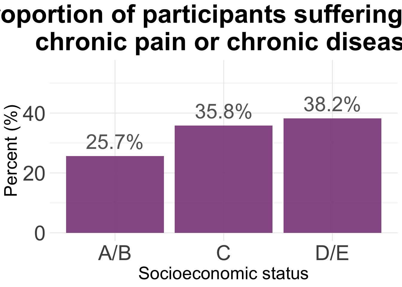

Version	Author	Date
c9896b1	Paloma	2025-02-25

#dev.off()

data <- m
# Step 1: Create a frequency table by SES and chronic condition
plot_data <- data %>%
  count(SES, chronic) %>%
  group_by(SES) %>%
  mutate(percent = 100 * n / sum(n))

# Step 2: Plot as grouped bar chart (percentage)
ggplot(plot_data, aes(x = SES, y = percent, fill = chronic)) +
  geom_bar(stat = "identity", position = "dodge") +
  scale_fill_manual(values = c("No" = "steelblue", "Yes" = "firebrick")) +
  labs(
    title = "Chronic Condition by Socioeconomic Status",
    x = "Socioeconomic Status",
    y = "Percentage",
    fill = "Chronic Condition"
  ) +
  theme_minimal(base_size = 13)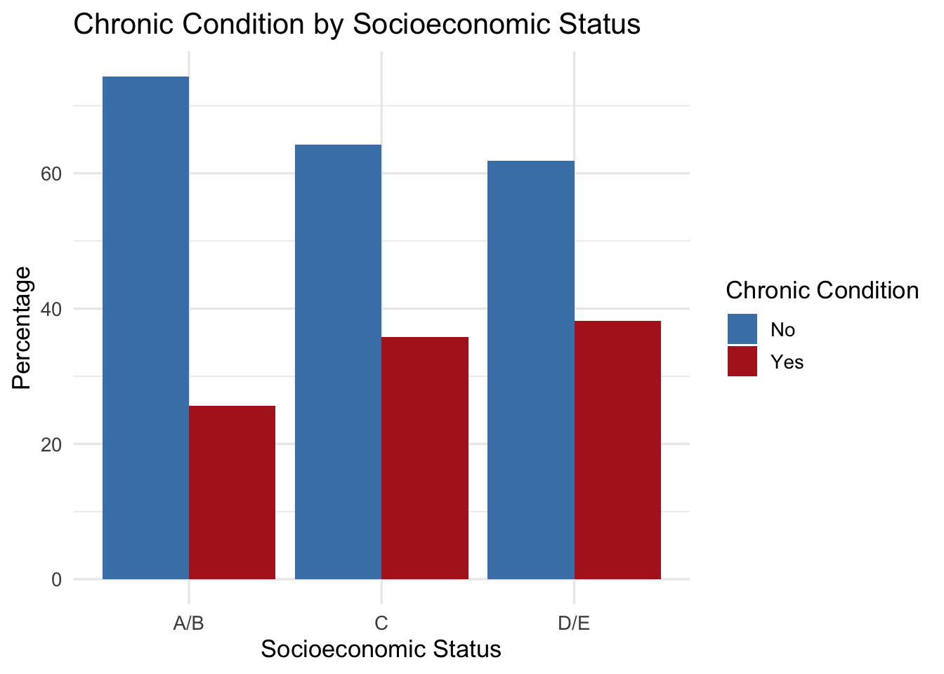

Version	Author	Date
3ca4968	Paloma	2025-04-10
c9896b1	Paloma	2025-02-25

models

# Sample dataframe (assumes it's already loaded as `data`)
data <- m
data$chronic <- factor(data$chronic, levels = c("No", "Yes"))
# Model 1: Overall SES score
m1 <- glm(chronic ~ SES_score, data = data, family = "binomial")

# Model 2: Overall SES category
m2 <- glm(chronic ~ SES, data = data, family = "binomial")

# Model 3: Individual SES components
m3 <- glm(chronic ~ SES_EDU_SC + SES_BTHR_SC + SES_CAR_SC + SES_INT_SC +
            SES_WRK_SC + SES_BEDR_SC, data = data, family = "binomial")

# Model 4: Components + categorical SES
m4 <- glm(chronic ~ SES + SES_EDU_SC + SES_BTHR_SC + SES_CAR_SC + SES_INT_SC +
            SES_WRK_SC + SES_BEDR_SC, data = data, family = "binomial")

# Model 5: SES components + interactions
m5 <- glm(chronic ~ SES_EDU_SC * SES_WRK_SC +
                    SES_BTHR_SC * SES_INT_SC +
                    SES_CAR_SC +
                    SES_BEDR_SC, 
          data = data, family = "binomial")

# Each model includes one SES component
m6 <- glm(chronic ~ SES_EDU_SC, data = data, family = "binomial")
m7 <- glm(chronic ~ SES_BTHR_SC, data = data, family = "binomial")
m8 <- glm(chronic ~ SES_CAR_SC, data = data, family = "binomial")
m9 <- glm(chronic ~ SES_INT_SC, data = data, family = "binomial")
m10 <- glm(chronic ~ SES_WRK_SC, data = data, family = "binomial")
m11 <- glm(chronic ~ SES_BEDR_SC, data = data, family = "binomial")
m12 <- glm(chronic ~ SES_EDU_SC + SES_BTHR_SC + SES_CAR_SC +
                     SES_INT_SC + SES_WRK_SC + SES_BEDR_SC,
           data = data, family = "binomial")


aic_table <- AIC(m1, m2, m3, m4, m5, m6, m7, m8, m9, m10 , m11, m12) %>%
  as.data.frame() %>%
  arrange(AIC)

print(aic_table)

    df      AIC
m7   2 443.9942
m11  2 444.5681
m1   2 446.9714
m2   3 447.9312
m8   2 448.4072
m10  2 448.4643
m3   7 448.7560
m12  7 448.7560
m9   2 448.7796
m6   2 449.2725
m5   9 451.2714
m4   9 452.0018

m7


Call:  glm(formula = chronic ~ SES_BTHR_SC, family = "binomial", data = data)

Coefficients:
(Intercept)  SES_BTHR_SC  
   -0.30351     -0.01602  

Degrees of Freedom: 345 Total (i.e. Null);  344 Residual
Null Deviance:      445.4 
Residual Deviance: 440  AIC: 444

m11


Call:  glm(formula = chronic ~ SES_BEDR_SC, family = "binomial", data = data)

Coefficients:
(Intercept)  SES_BEDR_SC  
   -0.04709     -0.04598  

Degrees of Freedom: 345 Total (i.e. Null);  344 Residual
Null Deviance:      445.4 
Residual Deviance: 440.6    AIC: 444.6

m4


Call:  glm(formula = chronic ~ SES + SES_EDU_SC + SES_BTHR_SC + SES_CAR_SC + 
    SES_INT_SC + SES_WRK_SC + SES_BEDR_SC, family = "binomial", 
    data = data)

Coefficients:
(Intercept)         SESC       SESD/E   SES_EDU_SC  SES_BTHR_SC   SES_CAR_SC  
  -1.131713     0.439617     0.478918     0.008199    -0.012825     0.001806  
 SES_INT_SC   SES_WRK_SC  SES_BEDR_SC  
   0.016794     0.005716    -0.038400  

Degrees of Freedom: 345 Total (i.e. Null);  337 Residual
Null Deviance:      445.4 
Residual Deviance: 434  AIC: 452

m1


Call:  glm(formula = chronic ~ SES_score, family = "binomial", data = data)

Coefficients:
(Intercept)    SES_score  
  -0.125478    -0.003945  

Degrees of Freedom: 345 Total (i.e. Null);  344 Residual
Null Deviance:      445.4 
Residual Deviance: 443  AIC: 447

best_model <- m7  # or whichever had lowest AIC

tidy_model <- tidy(best_model, conf.int = TRUE, exponentiate = TRUE) %>%
  filter(term != "(Intercept)")

ggplot(tidy_model, aes(x = reorder(term, estimate), y = estimate)) +
  geom_point(size = 4, color = "darkred") +
  geom_errorbar(aes(ymin = conf.low, ymax = conf.high), width = 0.2, color = "gray40") +
  geom_hline(yintercept = 1, linetype = "dashed", color = "gray60") +
  coord_flip() +
  labs(title = "Odds Ratios from Logistic Regression",
       subtitle = "Predicting Chronic Condition from SES Factors",
       x = "Predictor",
       y = "Odds Ratio (95% CI)") +
  theme_minimal(base_size = 13)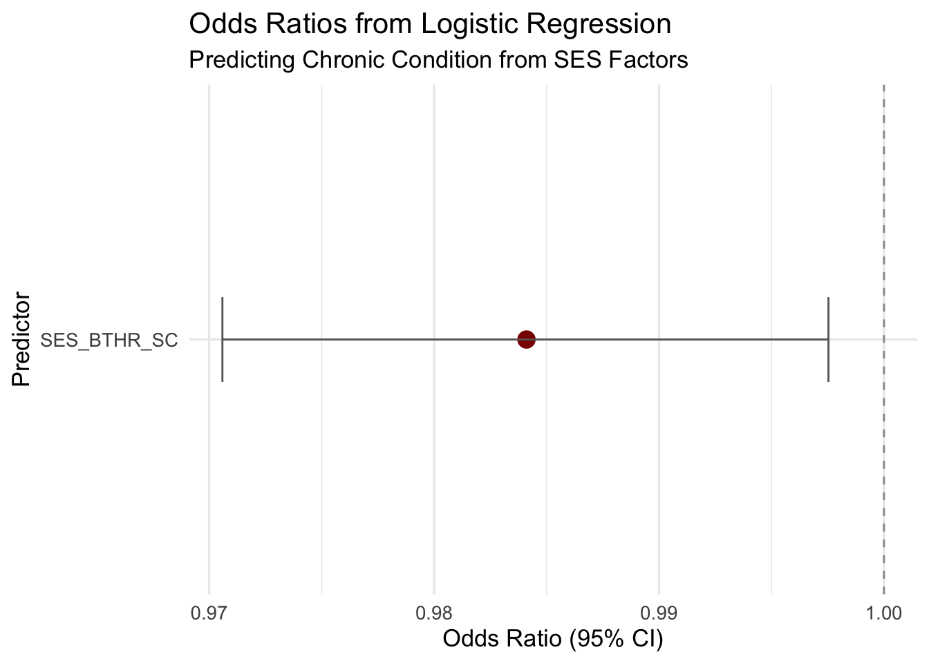

Version	Author	Date
3ca4968	Paloma	2025-04-10

SES and PSS - work in progress

f<-read.csv("./data/02.HWISE_PSS.csv")
# Add more info to file
dim(f)

[1] 398  33

f$ID <- as.factor(f$ID)

# Calculate total score PSS per participant
f$t_pss <- 0
# change positive statements to negative values
pss <- c(20, 21, 22, 23, 25, 26, 29)
for (i in pss) {f[i] <- f[i]*-1 }
    for (i in 1:nrow(f)) { 
    sum(f[i, c(18:31)]) -> f$Total_PSS[i]
}
summary(f$Total_PSS)

   Min. 1st Qu.  Median    Mean 3rd Qu.    Max.    NA's 
-13.000  -5.000  -2.000  -2.558   0.000   6.000       4

pss <- merge(m,f, by="ID")
dim(pss)

[1] 345  46

pss[pss =='NA'] <- NA

agg<- count(pss, SES, chronic, Total_PSS)
agg2 <- pivot_wider(agg, 
            names_from = chronic,
            values_from = n)
agg2$Total <- agg2$Yes/(agg2$Yes + agg2$No)*100

#png(file= "HLTH_counts_by_SES.png", width = 700, height = 800 )
ggplot(agg2, aes(x = SES, y = Total)) +
    geom_bar(stat= "identity", fill = "orchid4", alpha = 0.9) +
     ylim(0, 55) + 
   theme_minimal()  +
   geom_text(aes(label = paste(round(Total, 1), "%", sep="")), 
            vjust = -0.5, 
            colour = "gray40", 
            size = 9) +
   theme(
    plot.title = element_text(hjust = 0.5, 
                              size = 32, face = "bold"),
    axis.title = element_text(size = 22),  
    axis.text = element_text(size = 26)  
  ) + 
  labs(title="Proportion of participants suffering from \n chronic pain or chronic disease") +
  xlab("Socioeconomic status") +
  ylab("Percent (%)")

Warning: Removed 51 rows containing missing values or values outside the scale range
(`geom_bar()`).

Warning: Removed 24 rows containing missing values or values outside the scale range
(`geom_text()`).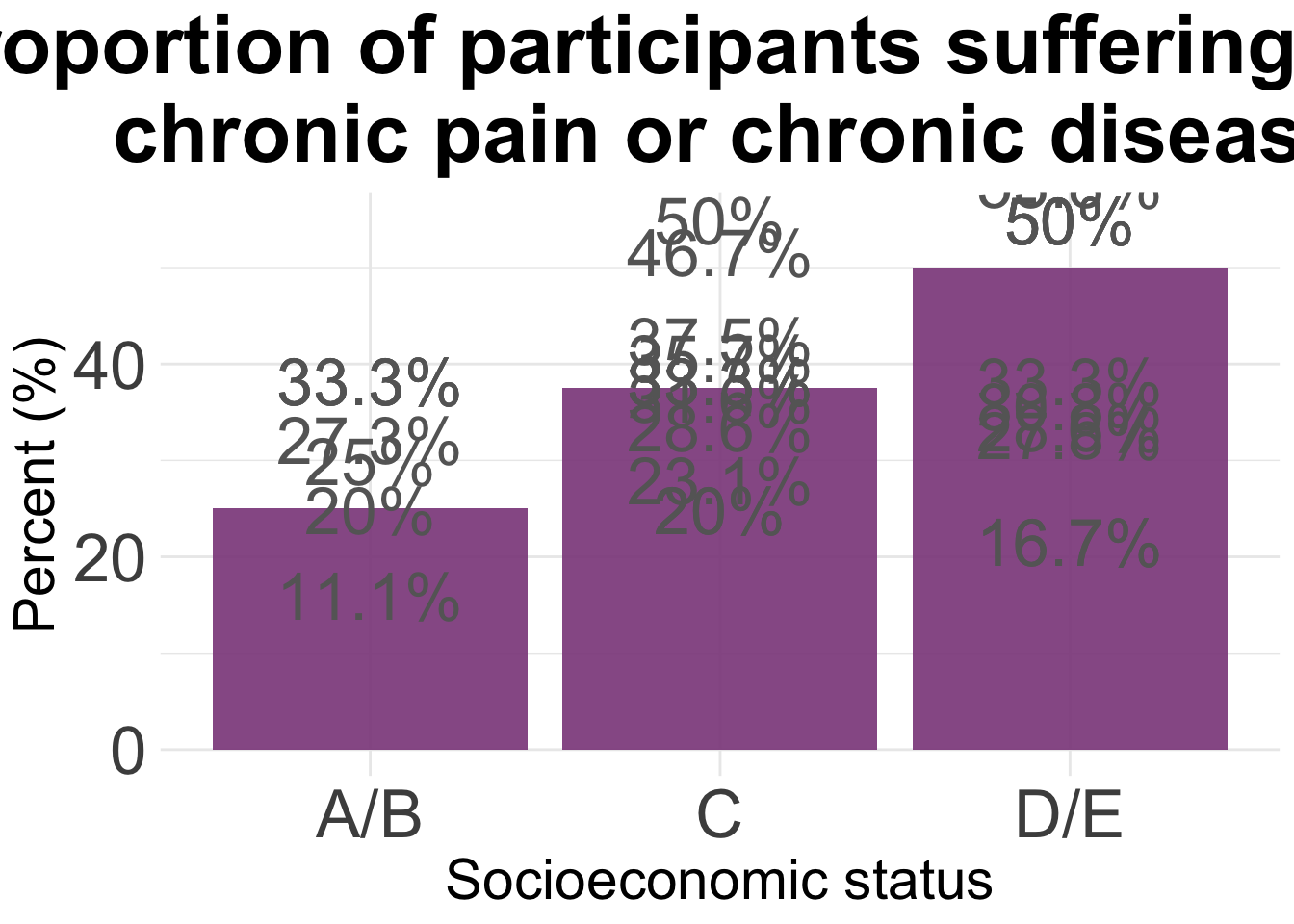

Version	Author	Date
3ca4968	Paloma	2025-04-10

#dev.off()

2. Create Combined Chronic Condition Variable

# Create binary variable: 1 = has chronic pain or disease
data <- df %>%
  mutate(chronic_any = ifelse(HLTH_CPAIN_CAT == 1 | HLTH_CDIS_CAT == 1, 1, 0)) %>%
  mutate(chronic_any = factor(chronic_any, labels = c("No chronic condition", "Chronic condition")))
data <- data %>% 
  filter(!is.na(chronic_any)) 
dim(data)

[1] 400  46

3. Descriptive stats

# Summary stats by chronic condition
data %>%
  group_by(chronic_any) %>%
  summarise(
    mean_pss = mean(PSS_TOTAL, na.rm = TRUE),
    sd_pss = sd(PSS_TOTAL, na.rm = TRUE),
    mean_ses = mean(SES_SC_Total, na.rm = TRUE),
    sd_ses = sd(SES_SC_Total, na.rm = TRUE),
    n = n()
  )

# A tibble: 2 × 6
  chronic_any          mean_pss sd_pss mean_ses sd_ses     n
  <fct>                   <dbl>  <dbl>    <dbl>  <dbl> <int>
1 No chronic condition   -1.42    7.35     136.   46.3   249
2 Chronic condition       0.436   6.82     127.   42.0   151

T-tests / Non-parametric Tests

# PSS comparison
wilcox.test(PSS_TOTAL ~ chronic_any, data = data)


    Wilcoxon rank sum test with continuity correction

data:  PSS_TOTAL by chronic_any
W = 15572, p-value = 0.01439
alternative hypothesis: true location shift is not equal to 0

# SES comparison
wilcox.test(SES_SC_Total ~ chronic_any, data = data)


    Wilcoxon rank sum test with continuity correction

data:  SES_SC_Total by chronic_any
W = 14914, p-value = 0.2122
alternative hypothesis: true location shift is not equal to 0

There is a statistically significant difference in stress levels between people with and without chronic conditions.

There is no statistically significant difference in SES between people with and without chronic conditions.

Visualizations: Boxplots

# Stress and SES by chronic condition
p1 <- ggplot(data, aes(x = chronic_any, y = PSS_TOTAL, fill = chronic_any)) +
  geom_point(aes(alpha = 0.8,  color = chronic_any), position = position_dodge2(width = 0.6)) +
  geom_violin(alpha = 0.3) +
  geom_boxplot(alpha = 0.8, width = 0.15) +
  labs(title = "Perceived Stress (PSS)", y = "PSS Score", x = NULL) +
  theme_minimal() +
  theme(legend.position = "none")

p2 <- ggplot(data, aes(x = chronic_any, y = SES_SC_Total, fill = chronic_any)) +
  geom_point(aes(alpha = 0.8,  color = chronic_any), position = position_dodge2(width = 0.6)) +
  geom_violin(alpha = 0.3) +
  geom_boxplot(alpha = 0.8, width = 0.15) +
  labs(title = "Socioeconomic Status", y = "SES Score", x = NULL) +
  theme_minimal() +
  theme(legend.position = "none")

# Combine plots
p1 + p2

Warning: Removed 6 rows containing non-finite outside the scale range
(`stat_ydensity()`).

Warning: Removed 6 rows containing non-finite outside the scale range
(`stat_boxplot()`).

Warning: Removed 6 rows containing missing values or values outside the scale range
(`geom_point()`).

Warning: Removed 51 rows containing non-finite outside the scale range
(`stat_ydensity()`).

Warning: Removed 51 rows containing non-finite outside the scale range
(`stat_boxplot()`).

Warning: Removed 51 rows containing missing values or values outside the scale range
(`geom_point()`).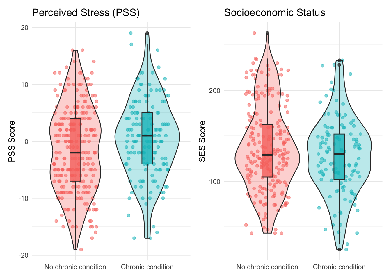

Version	Author	Date
3ca4968	Paloma	2025-04-10

Correlations

# Correlation matrix
cor_data <- data %>%
  select(PSS_TOTAL, SES_SC_Total, HW_TOTAL, D_AGE) %>%
  drop_na()

cor_matrix <- cor(cor_data)
corrplot(cor_matrix, method = "circle", type = "upper", tl.col = "black")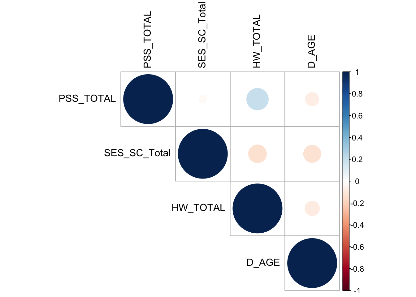

Version	Author	Date
3ca4968	Paloma	2025-04-10

Logistic Regression: Chronic condition ~ PSS + SES + Age

data <- data %>%
  mutate(chronic_any_binary = ifelse(chronic_any == "Chronic condition", 1, 0))

model <- glm(chronic_any_binary ~ PSS_TOTAL + SES_SC_Total + D_AGE, data = data, family = "binomial")

summary(model)


Call:
glm(formula = chronic_any_binary ~ PSS_TOTAL + SES_SC_Total + 
    D_AGE, family = "binomial", data = data)

Coefficients:
              Estimate Std. Error z value Pr(>|z|)  
(Intercept)  -1.416056   0.655860  -2.159   0.0308 *
PSS_TOTAL     0.035978   0.016141   2.229   0.0258 *
SES_SC_Total -0.003553   0.002618  -1.357   0.1747  
D_AGE         0.039526   0.015731   2.513   0.0120 *
---
Signif. codes:  0 '***' 0.001 '**' 0.01 '*' 0.05 '.' 0.1 ' ' 1

(Dispersion parameter for binomial family taken to be 1)

    Null deviance: 441.98  on 341  degrees of freedom
Residual deviance: 428.31  on 338  degrees of freedom
  (58 observations deleted due to missingness)
AIC: 436.31

Number of Fisher Scoring iterations: 4

exp(cbind(OR = coef(model), confint(model)))

Waiting for profiling to be done...

                    OR     2.5 %    97.5 %
(Intercept)  0.2426692 0.0660444 0.8692806
PSS_TOTAL    1.0366326 1.0046346 1.0704199
SES_SC_Total 0.9964535 0.9912834 1.0015363
D_AGE        1.0403180 1.0089896 1.0733125

Plot Odds Ratios

library(broom)
model_tidy <- tidy(model, conf.int = TRUE, exponentiate = TRUE)

ggplot(model_tidy, aes(x = reorder(term, estimate), y = estimate)) +
  geom_point(size = 4, color = "darkred") +
  geom_errorbar(aes(ymin = conf.low, ymax = conf.high), width = 0.2) +
  geom_hline(yintercept = 1, linetype = "dashed") +
  coord_flip() +
  labs(title = "Odds Ratios for Chronic Condition",
       x = "Predictor", y = "Odds Ratio (95% CI)") +
  theme_minimal()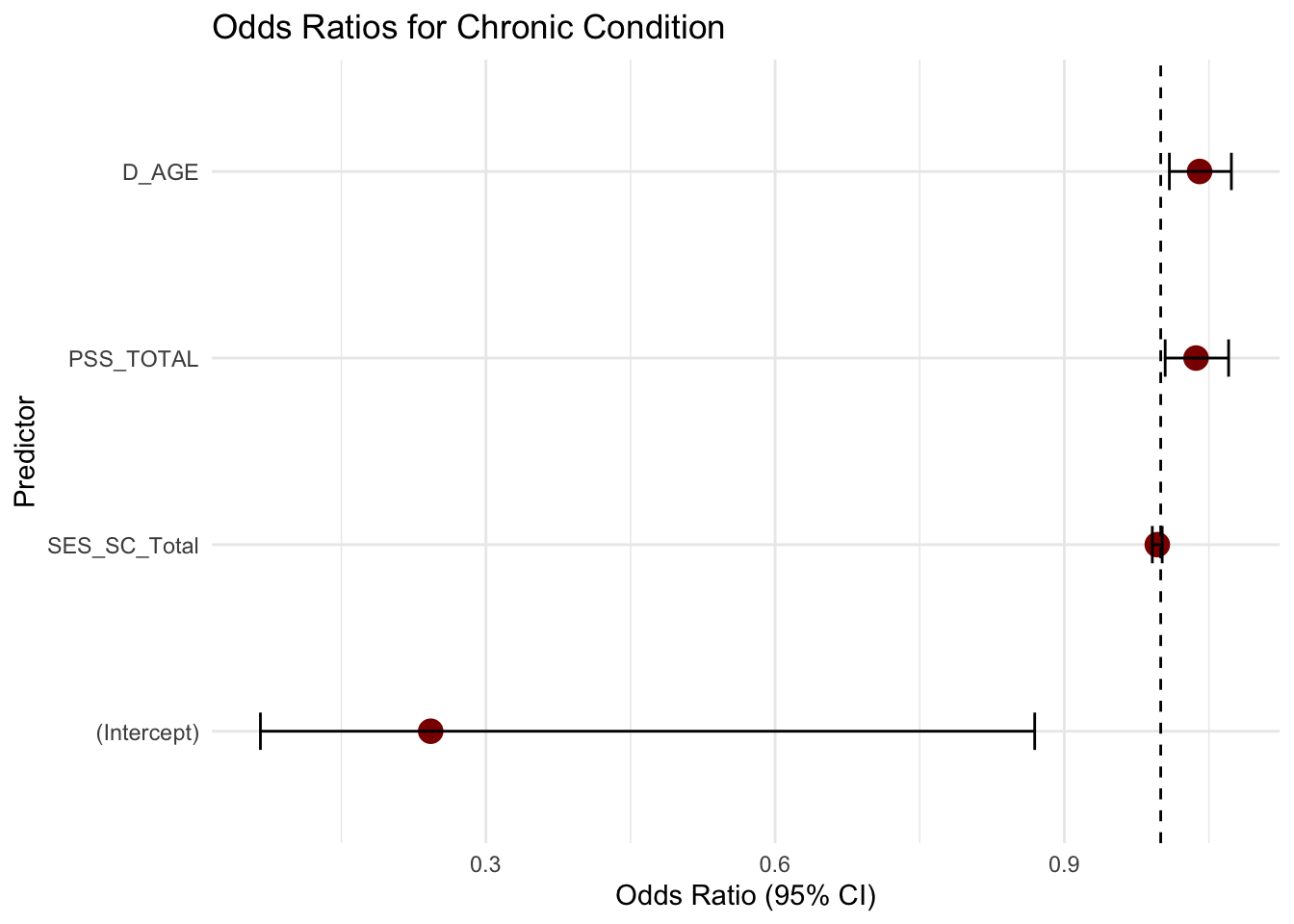

Version	Author	Date
3ca4968	Paloma	2025-04-10

Optional: Interaction Term (Stress × SES)

interaction_model <- glm(chronic_any_binary ~ PSS_TOTAL * SES_SC_Total + D_AGE,
                         data = data, family = "binomial")

summary(interaction_model)


Call:
glm(formula = chronic_any_binary ~ PSS_TOTAL * SES_SC_Total + 
    D_AGE, family = "binomial", data = data)

Coefficients:
                         Estimate Std. Error z value Pr(>|z|)   
(Intercept)            -1.4886649  0.6614362  -2.251  0.02441 * 
PSS_TOTAL              -0.0379014  0.0529489  -0.716  0.47411   
SES_SC_Total           -0.0033599  0.0026478  -1.269  0.20446   
D_AGE                   0.0409832  0.0158167   2.591  0.00957 **
PSS_TOTAL:SES_SC_Total  0.0005816  0.0003995   1.456  0.14540   
---
Signif. codes:  0 '***' 0.001 '**' 0.01 '*' 0.05 '.' 0.1 ' ' 1

(Dispersion parameter for binomial family taken to be 1)

    Null deviance: 441.98  on 341  degrees of freedom
Residual deviance: 426.15  on 337  degrees of freedom
  (58 observations deleted due to missingness)
AIC: 436.15

Number of Fisher Scoring iterations: 4

# Combine chronic pain + chronic disease
data <- data %>%
  mutate(chronic_any = ifelse(HLTH_CPAIN_CAT == 1 | HLTH_CDIS_CAT == 1, 1, 0),
         chronic_any = factor(chronic_any, levels = c(0,1)),
         chronic_any_binary = as.numeric(as.character(chronic_any)))  # for glm

# Model 1: Stress only
m1 <- glm(chronic_any_binary ~ PSS_TOTAL, data = data, family = "binomial")

# Model 2: SES only
m2 <- glm(chronic_any_binary ~ SES_SC_Total, data = data, family = "binomial")

# Model 3: Stress + SES
m3 <- glm(chronic_any_binary ~ PSS_TOTAL + SES_SC_Total, data = data, family = "binomial")

# Model 4: Add age
m4 <- glm(chronic_any_binary ~ PSS_TOTAL + SES_SC_Total + D_AGE, data = data, family = "binomial")

# Model 5: Add water insecurity
m5 <- glm(chronic_any_binary ~ PSS_TOTAL + SES_SC_Total + D_AGE + HW_TOTAL, data = data, family = "binomial")


AIC_table <- AIC(m1, m2, m3, m4, m5) %>%
  as.data.frame() %>%
  arrange(AIC)

Warning in AIC.default(m1, m2, m3, m4, m5): models are not all fitted to the
same number of observations

print(AIC_table)

   df      AIC
m5  5 428.2207
m4  4 436.3142
m3  3 442.2878
m2  2 451.5510
m1  2 520.3572

best_model <- m5  # or choose based on AIC_table

model_summary <- tidy(best_model, conf.int = TRUE, exponentiate = TRUE) %>%
  filter(term != "(Intercept)")

ggplot(model_summary, aes(x = reorder(term, estimate), y = estimate)) +
  geom_point(size = 4, color = "darkblue") +
  geom_errorbar(aes(ymin = conf.low, ymax = conf.high), width = 0.2) +
  geom_hline(yintercept = 1, linetype = "dashed", color = "gray60") +
  coord_flip() +
  labs(
    title = "Odds Ratios for Predicting Chronic Condition",
    subtitle = "Best model based on AIC",
    x = "Predictor",
    y = "Odds Ratio (95% CI)"
  ) +
  theme_minimal()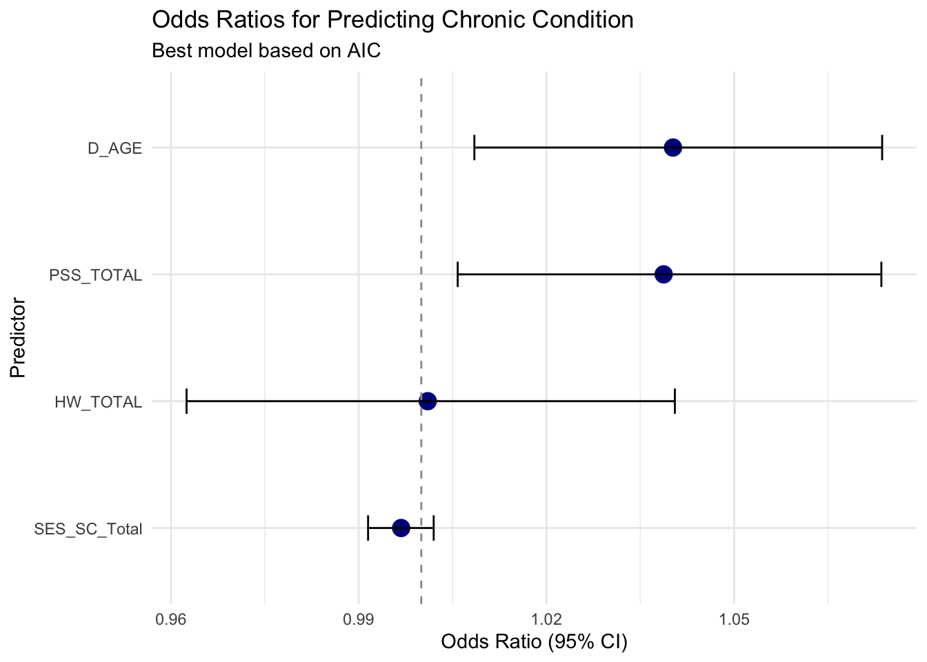

Version	Author	Date
3ca4968	Paloma	2025-04-10

# Interaction: Stress × SES
m_interact <- glm(chronic_any_binary ~ PSS_TOTAL * SES_SC_Total + D_AGE + HW_TOTAL,
                  data = data, family = "binomial")
summary(m_interact)


Call:
glm(formula = chronic_any_binary ~ PSS_TOTAL * SES_SC_Total + 
    D_AGE + HW_TOTAL, family = "binomial", data = data)

Coefficients:
                         Estimate Std. Error z value Pr(>|z|)  
(Intercept)            -1.5438055  0.7178573  -2.151   0.0315 *
PSS_TOTAL              -0.0269121  0.0536691  -0.501   0.6161  
SES_SC_Total           -0.0031297  0.0026976  -1.160   0.2460  
D_AGE                   0.0406790  0.0160154   2.540   0.0111 *
HW_TOTAL                0.0010111  0.0198194   0.051   0.9593  
PSS_TOTAL:SES_SC_Total  0.0005110  0.0004041   1.264   0.2061  
---
Signif. codes:  0 '***' 0.001 '**' 0.01 '*' 0.05 '.' 0.1 ' ' 1

(Dispersion parameter for binomial family taken to be 1)

    Null deviance: 431.78  on 335  degrees of freedom
Residual deviance: 416.60  on 330  degrees of freedom
  (64 observations deleted due to missingness)
AIC: 428.6

Number of Fisher Scoring iterations: 4

tidy_interact <- tidy(m_interact, conf.int = TRUE, exponentiate = TRUE) %>%
  filter(term != "(Intercept)")

ggplot(tidy_interact, aes(x = reorder(term, estimate), y = estimate)) +
  geom_point(size = 4, color = "darkred") +
  geom_errorbar(aes(ymin = conf.low, ymax = conf.high), width = 0.2) +
  geom_hline(yintercept = 1, linetype = "dashed", color = "gray60") +
  coord_flip() +
  labs(
    title = "Odds Ratios with Stress × SES Interaction",
    x = "Predictor",
    y = "Odds Ratio (95% CI)"
  ) +
  theme_minimal()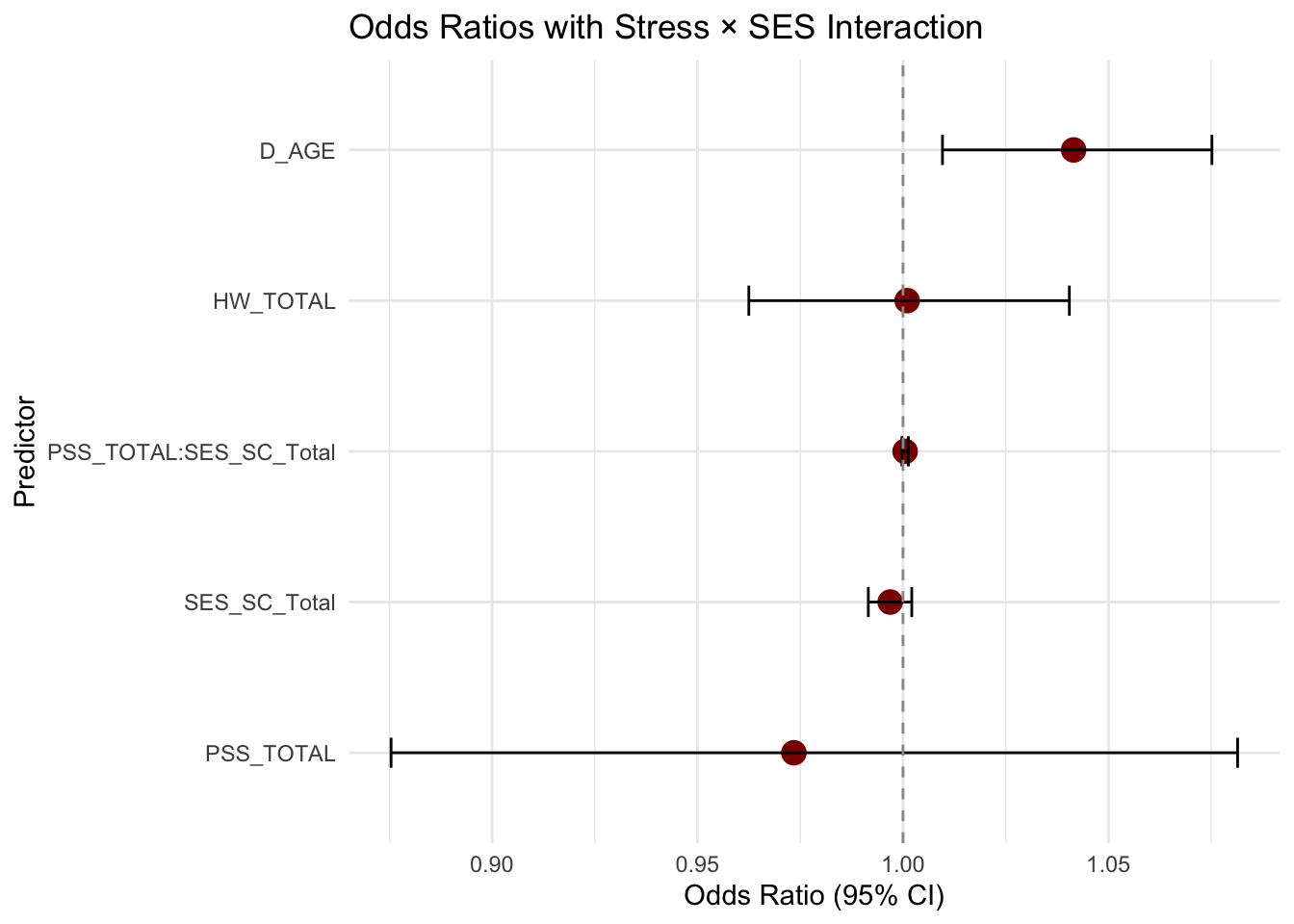

Version	Author	Date
3ca4968	Paloma	2025-04-10

# Create Predicted Probabilities Across SES Levels
#We’ll generate predicted probabilities of chronic condition at low, medium, and #high SES across a range of PSS (stress) values.

# Create a new data pr predictions
newdata <- expand.grid(
  PSS_TOTAL = seq(min(data$PSS_TOTAL, na.rm = TRUE),
                  max(data$PSS_TOTAL, na.rm = TRUE), length.out = 100),
  SES_SC_Total = quantile(data$SES_SC_Total, probs = c(0.25, 0.5, 0.75), na.rm = TRUE),
  D_AGE = mean(data$D_AGE, na.rm = TRUE),
  HW_TOTAL = mean(data$HW_TOTAL, na.rm = TRUE)
)

# Add a label for SES group
newdata$SES_group <- factor(newdata$SES_SC_Total,
                            labels = c("Low SES", "Medium SES", "High SES"))

# Predict probabilities
newdata$predicted <- predict(m_interact, newdata, type = "response")
ggplot(newdata, aes(x = PSS_TOTAL, y = predicted, color = SES_group)) +
  geom_line(size = 1.2) +
  labs(
    title = "Interaction of Stress and SES on Chronic Condition Risk",
    subtitle = "Predicted probability of chronic condition",
    x = "Perceived Stress Score",
    y = "Predicted Probability",
    color = "SES Level"
  ) +
  theme_minimal(base_size = 14) +
  scale_color_manual(values = c("Low SES" = "firebrick", "Medium SES" = "steelblue", "High SES" = "forestgreen")) +
  theme(legend.position = "top")

Warning: Using `size` aesthetic for lines was deprecated in ggplot2 3.4.0.
ℹ Please use `linewidth` instead.
This warning is displayed once every 8 hours.
Call `lifecycle::last_lifecycle_warnings()` to see where this warning was
generated.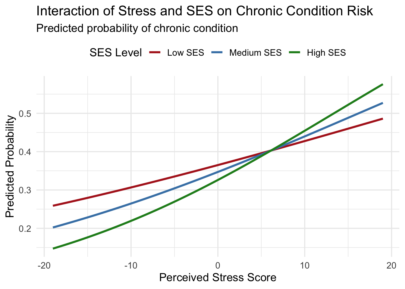

Version	Author	Date
3ca4968	Paloma	2025-04-10

sessionInfo()

R version 4.4.3 (2025-02-28)
Platform: aarch64-apple-darwin20
Running under: macOS Sequoia 15.4

Matrix products: default
BLAS:   /Library/Frameworks/R.framework/Versions/4.4-arm64/Resources/lib/libRblas.0.dylib 
LAPACK: /Library/Frameworks/R.framework/Versions/4.4-arm64/Resources/lib/libRlapack.dylib;  LAPACK version 3.12.0

locale:
[1] en_US.UTF-8/en_US.UTF-8/en_US.UTF-8/C/en_US.UTF-8/en_US.UTF-8

time zone: America/Detroit
tzcode source: internal

attached base packages:
[1] stats     graphics  grDevices utils     datasets  methods   base     

other attached packages:
[1] corrplot_0.95   patchwork_1.3.0 ggpubr_0.6.0    broom_1.0.7    
[5] tidyr_1.3.1     ggplot2_3.5.1   dplyr_1.1.4    

loaded via a namespace (and not attached):
 [1] sass_0.4.9        utf8_1.2.4        generics_0.1.3    rstatix_0.7.2    
 [5] stringi_1.8.4     digest_0.6.37     magrittr_2.0.3    evaluate_1.0.1   
 [9] grid_4.4.3        fastmap_1.2.0     rprojroot_2.0.4   workflowr_1.7.1  
[13] jsonlite_1.8.9    whisker_0.4.1     backports_1.5.0   Formula_1.2-5    
[17] promises_1.3.0    purrr_1.0.2       fansi_1.0.6       scales_1.3.0     
[21] jquerylib_0.1.4   abind_1.4-8       cli_3.6.3         crayon_1.5.3     
[25] rlang_1.1.4       munsell_0.5.1     withr_3.0.2       cachem_1.1.0     
[29] yaml_2.3.10       tools_4.4.3       ggsignif_0.6.4    colorspace_2.1-1 
[33] httpuv_1.6.15     vctrs_0.6.5       R6_2.5.1          lifecycle_1.0.4  
[37] git2r_0.35.0      stringr_1.5.1     car_3.1-3         fs_1.6.5         
[41] pkgconfig_2.0.3   pillar_1.9.0      bslib_0.8.0       later_1.3.2      
[45] gtable_0.3.6      glue_1.8.0        Rcpp_1.0.13-1     xfun_0.49        
[49] tibble_3.2.1      tidyselect_1.2.1  rstudioapi_0.17.1 knitr_1.49       
[53] farver_2.1.2      htmltools_0.5.8.1 labeling_0.4.3    carData_3.0-5    
[57] rmarkdown_2.29    compiler_4.4.3

Plots_Latinx_research_week

Paloma