Linear Regression Analysis
Junhui He, edited by Paloma C.
2025-03-07
Last updated: 2025-03-07
Checks: 6 1
Knit directory: QUAIL-Mex/
This reproducible R Markdown analysis was created with workflowr (version 1.7.1). The Checks tab describes the reproducibility checks that were applied when the results were created. The Past versions tab lists the development history.
The R Markdown file has unstaged changes. To know which version of
the R Markdown file created these results, you’ll want to first commit
it to the Git repo. If you’re still working on the analysis, you can
ignore this warning. When you’re finished, you can run
wflow_publish to commit the R Markdown file and build the
HTML.
Great job! The global environment was empty. Objects defined in the global environment can affect the analysis in your R Markdown file in unknown ways. For reproduciblity it’s best to always run the code in an empty environment.
The command set.seed(20241009) was run prior to running
the code in the R Markdown file. Setting a seed ensures that any results
that rely on randomness, e.g. subsampling or permutations, are
reproducible.
Great job! Recording the operating system, R version, and package versions is critical for reproducibility.
Nice! There were no cached chunks for this analysis, so you can be confident that you successfully produced the results during this run.
Great job! Using relative paths to the files within your workflowr project makes it easier to run your code on other machines.
Great! You are using Git for version control. Tracking code development and connecting the code version to the results is critical for reproducibility.
The results in this page were generated with repository version 4c407eb. See the Past versions tab to see a history of the changes made to the R Markdown and HTML files.
Note that you need to be careful to ensure that all relevant files for
the analysis have been committed to Git prior to generating the results
(you can use wflow_publish or
wflow_git_commit). workflowr only checks the R Markdown
file, but you know if there are other scripts or data files that it
depends on. Below is the status of the Git repository when the results
were generated:
Ignored files:
    Ignored:    .DS_Store
    Ignored:    .RData
    Ignored:    .Rhistory
    Ignored:    .Rproj.user/
    Ignored:    analysis/.DS_Store
    Ignored:    analysis/.RData
    Ignored:    analysis/.Rhistory
    Ignored:    code/.DS_Store
    Ignored:    data/.DS_Store

Untracked files:
    Untracked:  Cleaned_Dataset_Screening_HWISE_PSS_V2.csv
    Untracked:  analysis/Cleaned_Dataset_Screening_HWISE_PSS_V2.csv
    Untracked:  data/Filtered_Screening.csv

Unstaged changes:
    Modified:   analysis/HBA2025_Analyses.Rmd
    Modified:   analysis/HBA2025_cleaning.Rmd
    Modified:   analysis/MX28_plots.Rmd
    Modified:   analysis/Regression-Analysis_PC.Rmd
    Modified:   data/Cleaned_Dataset_Screening_HWISE_PSS_V3.csv
Note that any generated files, e.g. HTML, png, CSS, etc., are not included in this status report because it is ok for generated content to have uncommitted changes.
These are the previous versions of the repository in which changes were
made to the R Markdown
(analysis/Regression-Analysis_PC.Rmd) and HTML
(docs/Regression-Analysis_PC.html) files. If you’ve
configured a remote Git repository (see ?wflow_git_remote),
click on the hyperlinks in the table below to view the files as they
were in that past version.
| File | Version | Author | Date | Message |
|---|---|---|---|---|
| Rmd | 4ffe9ef | Junhui He | 2025-03-06 | add elastic-net |
| html | 4ffe9ef | Junhui He | 2025-03-06 | add elastic-net |
| Rmd | 0a00a41 | Paloma | 2025-03-06 | reg_analysis 2 |
| html | 0a00a41 | Paloma | 2025-03-06 | reg_analysis 2 |
| Rmd | 4a934f3 | Paloma | 2025-03-04 | incl research qs |
| html | 4a934f3 | Paloma | 2025-03-04 | incl research qs |
| Rmd | 6738718 | Paloma | 2025-03-04 | new regressions |
| html | 6738718 | Paloma | 2025-03-04 | new regressions |
| Rmd | f0811f0 | Paloma | 2025-03-04 | reduced NAs |
1 Introduction
Our research questions are:
What variables measured using Paloma’s questionnaires are good predictors of HWISE total scores?
What HWISE questions are good predictors of alternative water insecurity measurements, such as hours of water supply (HRS_WEEK), or type of supply (continuous or intermittent, W_WC_WI)?
Does water insecurity has any association with Perceived stress scores (PSS)? If so, what variables/aspects of water insecurity are driving this stress levels?
Here I repeat the analyses conducted by Junhui He, but adding and removing a few variables that could make more sense as predictors of the Total HWISE score or Total PSS score. These are the two linear regression models we run earlier:
HW_TOTAL ~ D_AGE + D_HH_SIZE + D_CHLD + HLTH_SMK + HLTH_CPAIN_CAT + HLTH_CDIS_CAT + SES_SC_Total
PSS_TOTAL ~ D_AGE + D_HH_SIZE + D_CHLD + HLTH_SMK + HLTH_CPAIN_CAT + HLTH_CDIS_CAT + SES_SC_Total
The two new linear regression models are different from the previous ones:
Removed HLTH_SMK, HLTH_CPAIN_CAT, and HLTH_CDIS_CAT
Added D_LOC_TIME, SEASON, W_WS_LOC, W_WC_WI, HRS_WEEK
Added HWISE_TOTAL as potential predictor of PSS
1.b Variable descriptions for quick reference
Ordered alphabetically
| Variable | Description | Class | Values |
|---|---|---|---|
| D_AGE | Participants’ age | Numeric | 18:49 |
| D_CHLD | Number of children participant has birthed | Numeric | 0:8 |
| D_HH_SIZE | Household size | Numeric | 2:40 |
| D_LOC_TIME | For how long have you lived in this neighborhood? | Numeric | 1:46 (years) |
| HLTH_CDIS_CAT | Presence of chronic disease | Categorical (Binary) | 1 = yes, 0 = no |
| HLTH_CPAIN_CAT | Presence of chronic pain | Categorical (Binary) | 1 = yes, 0 = no |
| HLTH_SMK | Tobacco smoker | Categorical (Binary) | 1 = yes, 0 = no |
| HRS_WEEK | Hours of water supply in the household per week | Numeric | 0:168 |
| HW_TOTAL | Sum of all 12-items in HWISE questionnaire | Numeric | 0:27 |
| MX28_WQ_COMP | Perception of water service as worse, same, or better than rest of Mexico City | Categorical (Ordinal) | 0 = worse, 1 = same, 2 = better |
| PSS_TOTAL | Total Perceived Stress Score | Numeric | -19:19 |
| SEASON | Fall or Spring (when data collection happened) | Categorical (Binary) | Fall = 1, Spring = 0 |
| SES_SC_Total | Socioeconomic status score | Numeric | 25:263 |
| W_WS_LOC | Classification of neighborhoods as water secure or insecure | Categorical (Binary) | 1 = water insecure, 0 = water secure |
| W_WC_WI | Classification of water supply as continuous or intermittent | Categorical (Binary) | 1 = intermittent, 0 = continuous |
2 Data preparation
We remove rows with missing data.
HW_TOTAL is calculated by adding up all the HWISE scores; PSS_TOTAL is calculated by adding up PSS 1,2,3, 8, 11, 12, 14, and substracting 4,5,6,7,9,10, and 13.
 [1] "ID"             "MX28_WQ_COMP"   "D_YRBR"         "D_LOC_TIME"
 [5] "D_AGE"          "D_HH_SIZE"      "D_CHLD"         "HLTH_SMK"
 [9] "SES_SC_Total"   "SEASON"         "W_WS_LOC"       "HW_WORRY"
[13] "HW_INTERR"      "HW_CLOTHES"     "HW_PLANS"       "HW_FOOD"
[17] "HW_HANDS"       "HW_BODY"        "HW_DRINK"       "HW_ANGRY"
[21] "HW_SLEEP"       "HW_NONE"        "HW_SHAME"       "PSS1"
[25] "PSS2"           "PSS3"           "PSS4"           "PSS5"
[29] "PSS6"           "PSS7"           "PSS8"           "PSS9"
[33] "PSS10"          "PSS11"          "PSS12"          "PSS13"
[37] "PSS14"          "HLTH_CPAIN_CAT" "HLTH_CDIS_CAT"  "HW_TOTAL"
[41] "W_WC_WI"        "HRS_WEEK"
Initial number of unique participants: 401 Initial number of variables: 42 | Variable | Missing_Values | |
|---|---|---|
| SES_SC_Total | SES_SC_Total | 52 |
| HRS_WEEK | HRS_WEEK | 39 |
| D_LOC_TIME | D_LOC_TIME | 36 |
| D_CHLD | D_CHLD | 24 |
| D_HH_SIZE | D_HH_SIZE | 23 |
| W_WC_WI | W_WC_WI | 22 |
| D_AGE | D_AGE | 18 |
| HW_TOTAL | HW_TOTAL | 11 |
| PSS_TOTAL | PSS_TOTAL | 7 |
| MX28_WQ_COMP | MX28_WQ_COMP | 4 |
| HLTH_CPAIN_CAT | HLTH_CPAIN_CAT | 4 |
| SEASON | SEASON | 3 |
| W_WS_LOC | W_WS_LOC | 3 |
| HLTH_CDIS_CAT | HLTH_CDIS_CAT | 1 |
| ID | ID | 0 |
Final number of unique participants: 258 Final number of variables: 15 List of variables: ID MX28_WQ_COMP D_LOC_TIME D_AGE D_HH_SIZE D_CHLD SES_SC_Total SEASON W_WS_LOC HLTH_CPAIN_CAT HLTH_CDIS_CAT HW_TOTAL W_WC_WI HRS_WEEK PSS_TOTAL3 Results
3.1 HWISE scores, variable set 1
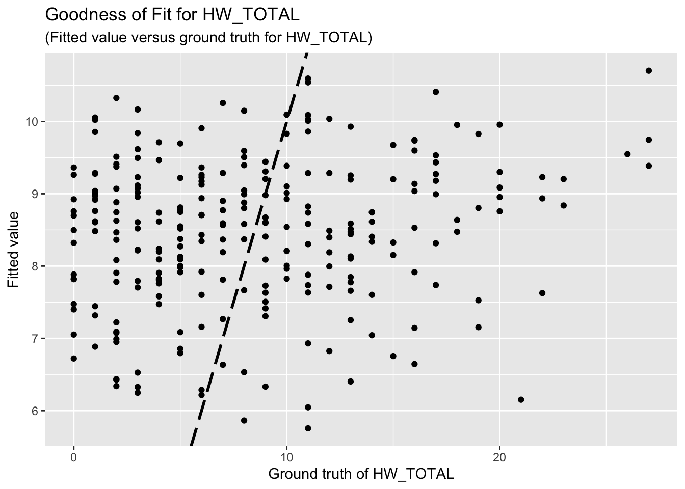
The regression results for HW is summarized as follows.
Call:
lm(formula = HW_TOTAL ~ D_AGE + D_HH_SIZE + D_CHLD + SES_SC_Total,
    data = reg_dataset)

Residuals:
    Min      1Q  Median      3Q     Max
-9.3640 -4.7302 -0.8448  4.3810 17.6134

Coefficients:
              Estimate Std. Error t value Pr(>|t|)
(Intercept)  13.492479   2.171256   6.214 2.11e-09 ***
D_AGE        -0.073610   0.057862  -1.272   0.2045
D_HH_SIZE    -0.077182   0.108093  -0.714   0.4759
D_CHLD        0.069070   0.355455   0.194   0.8461
SES_SC_Total -0.018128   0.009066  -2.000   0.0466 *
---
Signif. codes:  0 '***' 0.001 '**' 0.01 '*' 0.05 '.' 0.1 ' ' 1

Residual standard error: 6.141 on 253 degrees of freedom
Multiple R-squared:  0.0275,    Adjusted R-squared:  0.01213
F-statistic: 1.789 on 4 and 253 DF,  p-value: 0.1316
The goodness-of-fit for HW regression is given as follow.
| Version | Author | Date |
|---|---|---|
| 6738718 | Paloma | 2025-03-04 |
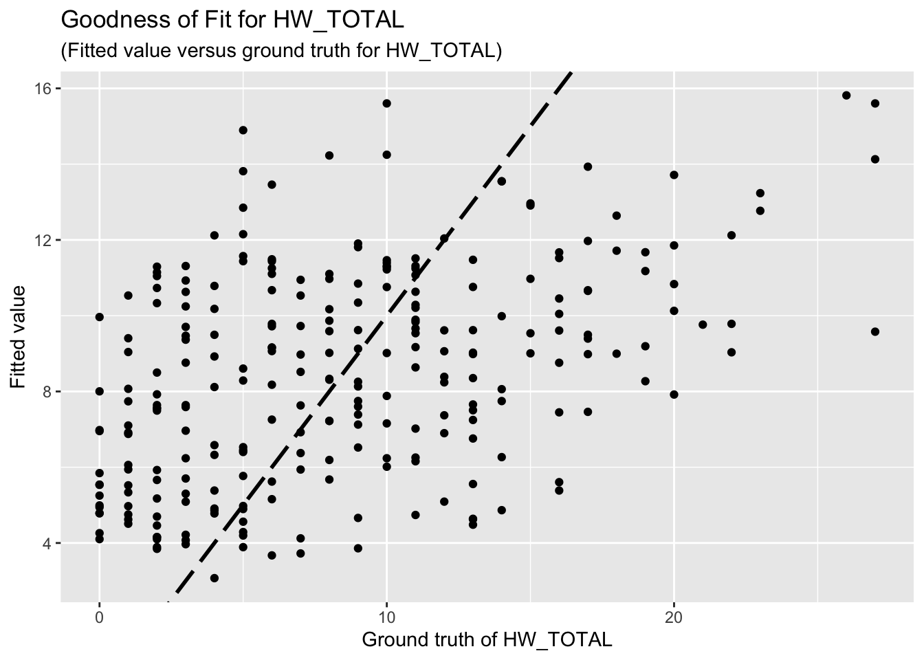
3.2 HWISE scores, variable set 2
Call:
lm(formula = HW_TOTAL ~ D_LOC_TIME + SEASON + W_WS_LOC + W_WC_WI +
    HRS_WEEK + D_AGE + D_HH_SIZE + D_CHLD + SES_SC_Total, data = reg_dataset)

Residuals:
    Min      1Q  Median      3Q     Max
-9.9644 -4.2574 -0.7626  3.9850 17.4225

Coefficients:
              Estimate Std. Error t value Pr(>|t|)
(Intercept)  15.751791   2.505217   6.288 1.44e-09 ***
D_LOC_TIME   -0.025907   0.033657  -0.770  0.44220
SEASON       -1.965150   0.777886  -2.526  0.01215 *
W_WS_LOC     -2.885457   1.027730  -2.808  0.00539 **
W_WC_WI       1.038550   1.110510   0.935  0.35059
HRS_WEEK     -0.040506   0.008797  -4.604 6.61e-06 ***
D_AGE         0.016391   0.058021   0.282  0.77780
D_HH_SIZE     0.007367   0.104940   0.070  0.94409
D_CHLD       -0.212119   0.326810  -0.649  0.51690
SES_SC_Total -0.011802   0.008421  -1.401  0.16233
---
Signif. codes:  0 '***' 0.001 '**' 0.01 '*' 0.05 '.' 0.1 ' ' 1

Residual standard error: 5.596 on 248 degrees of freedom
Multiple R-squared:  0.2087,    Adjusted R-squared:  0.1799
F-statistic: 7.266 on 9 and 248 DF,  p-value: 2.244e-09
The goodness-of-fit for HW regression is given as follow.
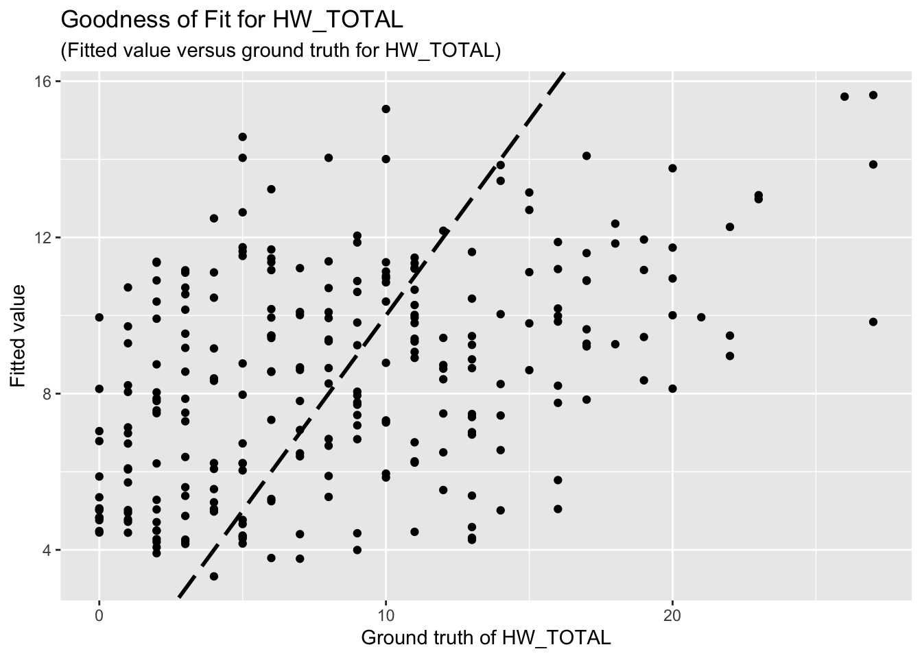
3.2 HWISE scores, variable set 3
Call:
lm(formula = HW_TOTAL ~ SEASON + W_WS_LOC + W_WC_WI + HRS_WEEK +
    D_AGE + D_HH_SIZE + D_CHLD + SES_SC_Total, data = reg_dataset)

Residuals:
    Min      1Q  Median      3Q     Max
-9.9523 -4.3187 -0.8347  4.0270 17.1629

Coefficients:
              Estimate Std. Error t value Pr(>|t|)
(Intercept)  15.777154   2.502949   6.303 1.31e-09 ***
SEASON       -1.899639   0.772582  -2.459  0.01462 *
W_WS_LOC     -2.946993   1.023777  -2.879  0.00434 **
W_WC_WI       1.053722   1.109426   0.950  0.34314
HRS_WEEK     -0.040974   0.008769  -4.673 4.87e-06 ***
D_AGE         0.002589   0.055136   0.047  0.96258
D_HH_SIZE     0.004810   0.104801   0.046  0.96343
D_CHLD       -0.212761   0.326541  -0.652  0.51529
SES_SC_Total -0.012682   0.008336  -1.521  0.12943
---
Signif. codes:  0 '***' 0.001 '**' 0.01 '*' 0.05 '.' 0.1 ' ' 1

Residual standard error: 5.591 on 249 degrees of freedom
Multiple R-squared:  0.2068,    Adjusted R-squared:  0.1813
F-statistic: 8.113 on 8 and 249 DF,  p-value: 9.783e-10
The goodness-of-fit for HW regression is given as follow.
| Version | Author | Date |
|---|---|---|
| 0a00a41 | Paloma | 2025-03-06 |
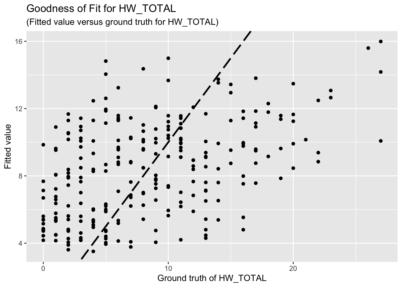
3.2 HWISE scores, variable set 4
Call:
lm(formula = HW_TOTAL ~ MX28_WQ_COMP + SEASON + W_WS_LOC + W_WC_WI +
    HRS_WEEK + D_CHLD + SES_SC_Total, data = reg_dataset)

Residuals:
    Min      1Q  Median      3Q     Max
-9.9025 -4.3628 -0.6919  3.9573 16.9225

Coefficients:
              Estimate Std. Error t value Pr(>|t|)
(Intercept)  16.246554   2.124773   7.646 4.45e-13 ***
MX28_WQ_COMP -0.309043   0.462558  -0.668  0.50468
SEASON       -1.917502   0.710432  -2.699  0.00743 **
W_WS_LOC     -3.014026   1.021080  -2.952  0.00346 **
W_WC_WI       0.990233   1.110034   0.892  0.37321
HRS_WEEK     -0.040752   0.008728  -4.669 4.94e-06 ***
D_CHLD       -0.194804   0.287616  -0.677  0.49884
SES_SC_Total -0.013073   0.008166  -1.601  0.11066
---
Signif. codes:  0 '***' 0.001 '**' 0.01 '*' 0.05 '.' 0.1 ' ' 1

Residual standard error: 5.575 on 250 degrees of freedom
Multiple R-squared:  0.2082,    Adjusted R-squared:  0.186
F-statistic: 9.389 on 7 and 250 DF,  p-value: 2.478e-10
The goodness-of-fit for HW regression is given as follow.
| Version | Author | Date |
|---|---|---|
| 0a00a41 | Paloma | 2025-03-06 |
3.3 PSS
The regression results for PSS is summarized as follows.
Call:
lm(formula = PSS_TOTAL ~ D_LOC_TIME + MX28_WQ_COMP + SEASON +
W_WS_LOC + W_WC_WI + HRS_WEEK + D_AGE + D_HH_SIZE + D_CHLD +
SES_SC_Total + HW_TOTAL, data = reg_dataset)
Residuals:
Min 1Q Median 3Q Max
-20.3872 -4.5990 -0.0205 5.5707 18.9758
Coefficients:
Estimate Std. Error t value Pr(>|t|)
(Intercept) -3.461375 3.651567 -0.948 0.3441
D_LOC_TIME -0.049297 0.043971 -1.121 0.2633
MX28_WQ_COMP 1.248716 0.614027 2.034 0.0431 *
SEASON 0.564774 1.021724 0.553 0.5809
W_WS_LOC 0.855484 1.359292 0.629 0.5297
W_WC_WI 1.270821 1.446354 0.879 0.3805
HRS_WEEK 0.008148 0.011878 0.686 0.4934
D_AGE -0.074931 0.076227 -0.983 0.3266
D_HH_SIZE -0.162582 0.136094 -1.195 0.2334
D_CHLD 0.696026 0.425757 1.635 0.1034
SES_SC_Total 0.005177 0.011023 0.470 0.6390
HW_TOTAL 0.209864 0.082314 2.550 0.0114 *
---
Signif. codes: 0 '***' 0.001 '**' 0.01 '*' 0.05 '.' 0.1 ' ' 1
Residual standard error: 7.248 on 246 degrees of freedom
Multiple R-squared: 0.07158, Adjusted R-squared: 0.03006
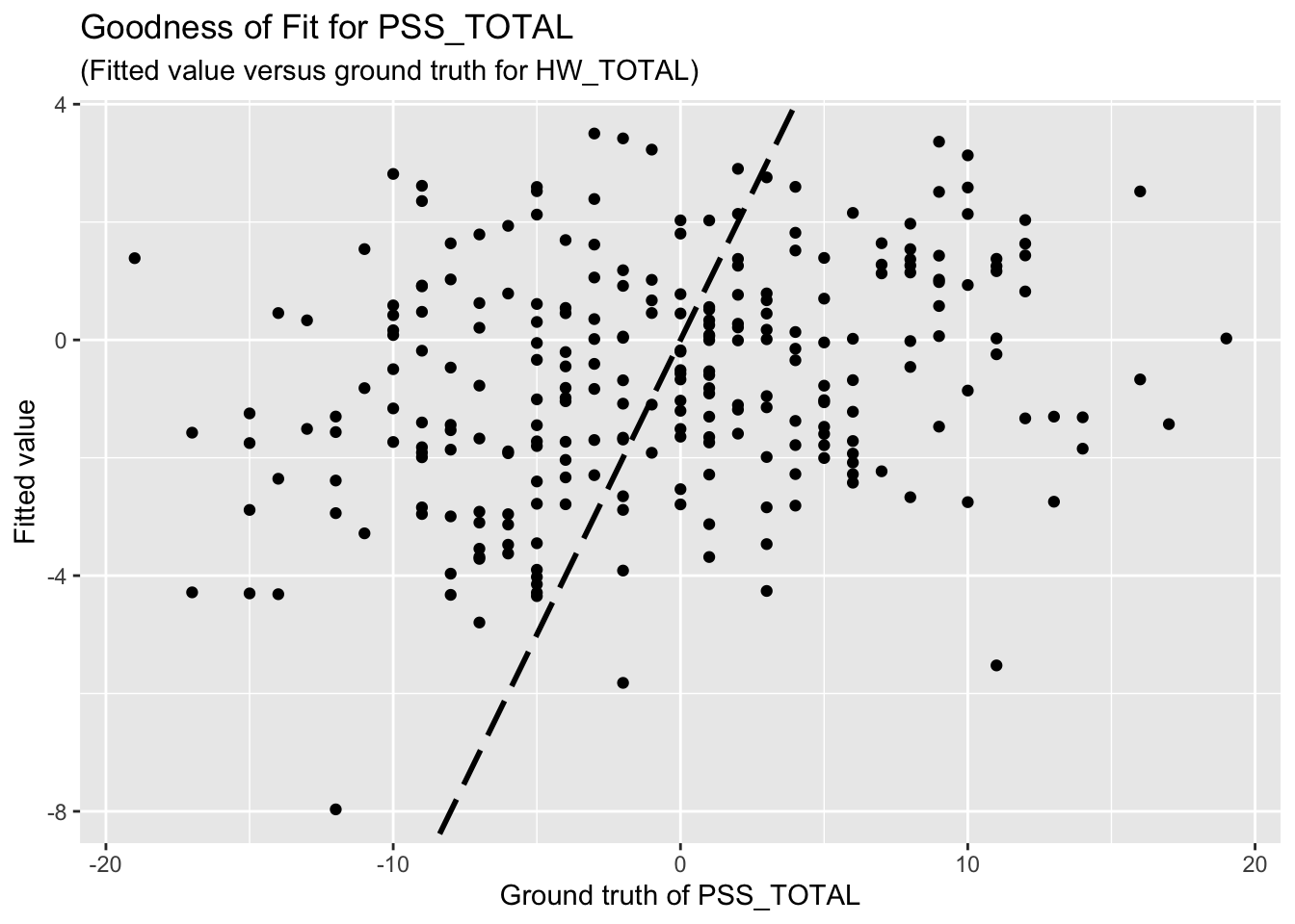
F-statistic: 1.724 on 11 and 246 DF, p-value: 0.06864The goodness-of-fit for PSS regression is given as follow.
3.4 Predictors for hours of water supply
WORK IN PROGRESS I intend to add each HWISE question in these models
Call:
lm(formula = HRS_WEEK ~ MX28_WQ_COMP + D_LOC_TIME + SEASON +
W_WS_LOC + W_WC_WI + HW_TOTAL + D_AGE + D_HH_SIZE + D_CHLD +
SES_SC_Total, data = reg_dataset)
Residuals:
Min 1Q Median 3Q Max
-119.11 -16.31 -3.97 10.80 140.72
Coefficients:
Estimate Std. Error t value Pr(>|t|)
(Intercept) 170.40992 16.28102 10.467 < 2e-16 ***
MX28_WQ_COMP 1.49846 3.28792 0.456 0.649
D_LOC_TIME 0.18017 0.23527 0.766 0.445
SEASON 4.60873 5.46544 0.843 0.400
W_WS_LOC -63.16290 6.07208 -10.402 < 2e-16 ***
W_WC_WI -61.43394 6.68969 -9.183 < 2e-16 ***
HW_TOTAL -1.93529 0.42341 -4.571 7.69e-06 ***
D_AGE 0.12601 0.40826 0.309 0.758
D_HH_SIZE -0.61571 0.72799 -0.846 0.399
D_CHLD -1.26464 2.27933 -0.555 0.580
SES_SC_Total 0.00536 0.05905 0.091 0.928
---
Signif. codes: 0 '***' 0.001 '**' 0.01 '*' 0.05 '.' 0.1 ' ' 1
Residual standard error: 38.83 on 247 degrees of freedom
Multiple R-squared: 0.7047, Adjusted R-squared: 0.6928
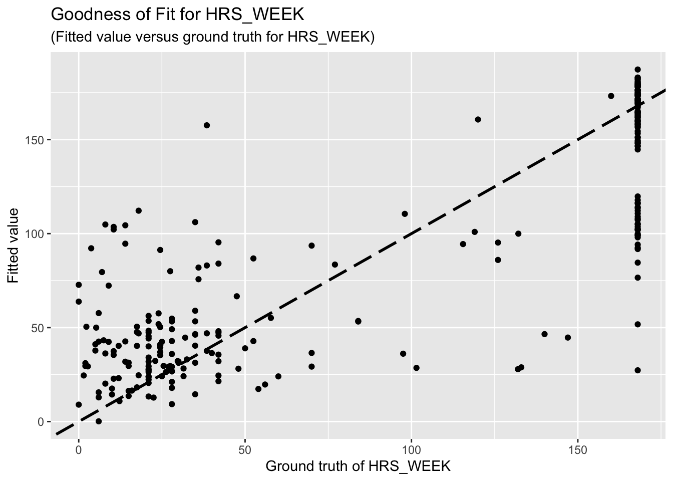
F-statistic: 58.95 on 10 and 247 DF, p-value: < 2.2e-16The goodness-of-fit for HW regression is given as follow.
| Version | Author | Date |
|---|---|---|
| 0a00a41 | Paloma | 2025-03-06 |
3.5 Predictors for perception of W. supply as better, same or worse
WORK IN PROGRESS –> outcome variable is categorical, can’t be runned as other vars
4 Feature selection
Using Elastic-Net Algorithm with \(\alpha=0.5\), the selected predictors for HW_TOTAL include D_LOC_TIME, D_CHILD, SES_SC_TOTAL, SEASON, W_WS_LOC, W_WC_WI, and HRS_WEEK.
10 x 1 sparse Matrix of class "dgCMatrix"
                        s0
(Intercept)    11.63669848
MX28_WQ_COMP   -0.42887671
D_LOC_TIME     -0.01987728
D_AGE           .
D_HH_SIZE       .
D_CHLD          .
SES_SC_Total   -0.01015526
SEASON         -1.94496389
HLTH_CPAIN_CAT  .
HLTH_CDIS_CAT   .
11 x 1 sparse Matrix of class "dgCMatrix"
s0
(Intercept) 0.03044184
MX28_WQ_COMP 0.90710902
D_LOC_TIME -0.04358665
D_AGE -0.06140550
D_HH_SIZE -0.06672025
D_CHLD 0.55366553
SES_SC_Total .
SEASON .
W_WS_LOC 0.55262337
HLTH_CPAIN_CAT 0.62284421
HLTH_CDIS_CAT 2.184814505 Discussion
5.2 Questions
Is it reasonable to use HW_TOTAL or PSS_TOTAL as response variables and other aforementioned variables as predictors? If not, how should I choose response variables and predictors?
Previously, I mentioned feature selection, a method used to identify the most influential variables among a set of predictors. Here, “the most influential variable” refers to one that has a significant impact on the response. However, since your cleaned dataset contains only eight predictors, I believe feature selection is unnecessary. Moreover, feature selection is typically employed to prevent overfitting, whereas our primary problem is underfitting.
R version 4.4.3 (2025-02-28)
Platform: aarch64-apple-darwin20
Running under: macOS Sequoia 15.3.1

Matrix products: default
BLAS:   /Library/Frameworks/R.framework/Versions/4.4-arm64/Resources/lib/libRblas.0.dylib
LAPACK: /Library/Frameworks/R.framework/Versions/4.4-arm64/Resources/lib/libRlapack.dylib;  LAPACK version 3.12.0

locale:
[1] en_US.UTF-8/en_US.UTF-8/en_US.UTF-8/C/en_US.UTF-8/en_US.UTF-8

time zone: America/Detroit
tzcode source: internal

attached base packages:
[1] stats     graphics  grDevices utils     datasets  methods   base

other attached packages:
[1] knitr_1.49    glmnet_4.1-8  Matrix_1.7-2  naniar_1.1.0  ggplot2_3.5.1
[6] mice_3.17.0   dplyr_1.1.4

loaded via a namespace (and not attached):
 [1] gtable_0.3.6      shape_1.4.6.1     xfun_0.49         bslib_0.8.0
 [5] visdat_0.6.0      lattice_0.22-6    vctrs_0.6.5       tools_4.4.3
 [9] Rdpack_2.6.2      generics_0.1.3    tibble_3.2.1      fansi_1.0.6
[13] pan_1.9           pkgconfig_2.0.3   jomo_2.7-6        lifecycle_1.0.4
[17] farver_2.1.2      compiler_4.4.3    stringr_1.5.1     git2r_0.35.0
[21] munsell_0.5.1     codetools_0.2-20  httpuv_1.6.15     htmltools_0.5.8.1
[25] sass_0.4.9        yaml_2.3.10       later_1.3.2       pillar_1.9.0
[29] nloptr_2.1.1      jquerylib_0.1.4   whisker_0.4.1     tidyr_1.3.1
[33] MASS_7.3-64       cachem_1.1.0      reformulas_0.4.0  iterators_1.0.14
[37] rpart_4.1.24      boot_1.3-31       foreach_1.5.2     mitml_0.4-5
[41] nlme_3.1-167      tidyselect_1.2.1  digest_0.6.37     stringi_1.8.4
[45] purrr_1.0.2       labeling_0.4.3    splines_4.4.3     rprojroot_2.0.4
[49] fastmap_1.2.0     grid_4.4.3        colorspace_2.1-1  cli_3.6.3
[53] magrittr_2.0.3    survival_3.8-3    utf8_1.2.4        broom_1.0.7
[57] withr_3.0.2       scales_1.3.0      promises_1.3.0    backports_1.5.0
[61] rmarkdown_2.29    nnet_7.3-20       lme4_1.1-36       workflowr_1.7.1
[65] evaluate_1.0.1    rbibutils_2.3     rlang_1.1.4       Rcpp_1.0.13-1
[69] glue_1.8.0        rstudioapi_0.17.1 minqa_1.2.8       jsonlite_1.8.9
[73] R6_2.5.1          fs_1.6.5
5.1 Comments on results
Unfortunately, the coefficient estimates are not significant except for a few predictors. This indicates the linear dependency between the response (HW_TOTAL or PSS_TOTAL) and the predictors are not significant.
Based on the goodness-of-fit figures, the predictive performance is really bad, which is consistent with the last comment.