data_modeling_1
calliquire
2024-10-03
Last updated: 2024-10-07
Checks: 6 1
Knit directory: SAPPHIRE/
This reproducible R Markdown analysis was created with workflowr (version 1.7.1). The Checks tab describes the reproducibility checks that were applied when the results were created. The Past versions tab lists the development history.
The R Markdown file has unstaged changes. To know which version of
the R Markdown file created these results, you’ll want to first commit
it to the Git repo. If you’re still working on the analysis, you can
ignore this warning. When you’re finished, you can run
wflow_publish to commit the R Markdown file and build the
HTML.
Great job! The global environment was empty. Objects defined in the global environment can affect the analysis in your R Markdown file in unknown ways. For reproduciblity it’s best to always run the code in an empty environment.
The command set.seed(20240923) was run prior to running
the code in the R Markdown file. Setting a seed ensures that any results
that rely on randomness, e.g. subsampling or permutations, are
reproducible.
Great job! Recording the operating system, R version, and package versions is critical for reproducibility.
Nice! There were no cached chunks for this analysis, so you can be confident that you successfully produced the results during this run.
Great job! Using relative paths to the files within your workflowr project makes it easier to run your code on other machines.
Great! You are using Git for version control. Tracking code development and connecting the code version to the results is critical for reproducibility.
The results in this page were generated with repository version bcfeb36. See the Past versions tab to see a history of the changes made to the R Markdown and HTML files.
Note that you need to be careful to ensure that all relevant files for
the analysis have been committed to Git prior to generating the results
(you can use wflow_publish or
wflow_git_commit). workflowr only checks the R Markdown
file, but you know if there are other scripts or data files that it
depends on. Below is the status of the Git repository when the results
were generated:
Ignored files:
    Ignored:    .DS_Store
    Ignored:    .Rapp.history
    Ignored:    .Rhistory
    Ignored:    .Rproj.user/
    Ignored:    analysis/.DS_Store
    Ignored:    data/.DS_Store

Unstaged changes:
    Modified:   analysis/data_modeling_1.Rmd
Note that any generated files, e.g. HTML, png, CSS, etc., are not included in this status report because it is ok for generated content to have uncommitted changes.
These are the previous versions of the repository in which changes were
made to the R Markdown (analysis/data_modeling_1.Rmd) and
HTML (docs/data_modeling_1.html) files. If you’ve
configured a remote Git repository (see ?wflow_git_remote),
click on the hyperlinks in the table below to view the files as they
were in that past version.
| File | Version | Author | Date | Message |
|---|---|---|---|---|
| Rmd | 596dc6e | calliquire | 2024-10-07 | More plot editing |
| html | 596dc6e | calliquire | 2024-10-07 | More plot editing |
| Rmd | 97aea45 | calliquire | 2024-10-07 | doing the linear mixed effects model |
| html | 97aea45 | calliquire | 2024-10-07 | doing the linear mixed effects model |
| Rmd | d720809 | calliquire | 2024-10-07 | edit relevant columns for analysis |
| Rmd | f6f08f1 | calliquire | 2024-10-07 | editing data modeling |
| Rmd | fdf9a11 | calliquire | 2024-10-04 | edited plots |
| html | fdf9a11 | calliquire | 2024-10-04 | edited plots |
| Rmd | 4745967 | calliquire | 2024-10-03 | added save step |
| html | 4745967 | calliquire | 2024-10-03 | added save step |
| Rmd | 572131a | calliquire | 2024-10-03 | baby’s first data vis |
| html | 572131a | calliquire | 2024-10-03 | baby’s first data vis |
| Rmd | e0261c4 | calliquire | 2024-10-03 | Create data_modeling_1.Rmd |
About This Analysis: The goal of this analysis is to fit a Linear Mixed Effects Model to the cleaned and filtered data set.
Purpose of the Model: The linear mixed-effects model aims to predict the reflectance values while accounting for both fixed effects (collection periods and reflectance metrics) and random effects (individual differences among participants). This is especially useful in repeated measures data, where you want to understand how specific factors influence the response while considering individual variability.
Fixed Effects Interpretation: The fixed effects coefficients will tell you:
How much the reflectance value changes with different collection periods, holding the reflectance metric constant.
How much the reflectance value changes with different reflectance metrics, holding the collection period constant. - How the relationship between reflectance values and collection period varies for different metrics.
Random Effects Interpretation: The random effects component allows you to model the inherent variability between participants. For example, if one participant consistently has higher reflectance values than another, the model accounts for that difference.
Set Up
- Load the data.
data <- read.csv("data/screening_data/filtered_screening_long.csv")- Load relevant libraries.
library(ggstatsplot)
library(ggplot2)
library(ggeffects)
library(dplyr)
library(viridis)
library(lme4)
Linear Mixed Effects Modeling
- Convert the categorical columns into factors.
data$collection_period <- factor(data$collection_period, levels = c("Summer", "Winter", "6Weeks"))
data$reflectance_metric <- as.factor(data$reflectance_metric)- Fit the Linear Mixed Effects Model.
An overview of this model:
Response Variable:
- reflectance_value: This is the dependent variable (response) that you are trying to predict or explain. It represents the measured reflectance values from the different metrics across various collection periods.
Fixed Effects:
collection_period: This is a categorical independent variable that denotes different time periods when the measurements were taken (e.g., Summer, Winter, and 6 Weeks). It helps in examining how reflectance values vary across these periods.
reflectance_metric: This is another categorical independent variable representing different types of reflectance metrics (e.g., e1, e2, m1, etc.). It helps assess how the type of metric influences reflectance values.
collection_period * reflectance_metric: The asterisk (*) indicates that you are including both main effects (collection period and reflectance metric) and their interaction. This allows you to see not only the individual effects of each variable but also how the effect of one variable depends on the level of the other (e.g., how the relationship between reflectance values and collection period changes across different metrics).
Random Effects:
(1 | participant_centre_id): This part of the model specifies a random intercept for participants. Here, participant_centre_id is the grouping variable representing individual participants (or centres, depending on the context). By including this random effect:
You allow for individual differences in the baseline level of reflectance values. Each participant can have their own average reflectance value, accounting for natural variability between participants.
The model captures correlations in reflectance values within the same participant, given that repeated measurements are taken on each individual.
model <- lmer(reflectance_value ~ collection_period * reflectance_metric + (1 | participant_centre_id), data = data)

# Summarize the model
summary(model)
Linear mixed model fit by REML ['lmerMod']
Formula: reflectance_value ~ collection_period * reflectance_metric +
(1 | participant_centre_id)
Data: data
REML criterion at convergence: 121836.4
Scaled residuals:
Min 1Q Median 3Q Max
-7.1287 -0.4258 0.0110 0.3332 16.0660
Random effects:
Groups Name Variance Std.Dev.
participant_centre_id (Intercept) 37.92 6.158
Residual 148.43 12.183
Number of obs: 15521, groups: participant_centre_id, 103
Fixed effects:
Estimate Std. Error t value
(Intercept) 12.95029 0.92115 14.059
collection_periodWinter -0.05200 1.03620 -0.050
collection_period6Weeks 3.19209 1.44957 2.202
reflectance_metrica_2 0.01120 0.98017 0.011
reflectance_metrica_3 0.04799 0.98017 0.049
reflectance_metricb_1 -0.57414 0.98017 -0.586
reflectance_metricb_2 -0.79777 0.98017 -0.814
reflectance_metricb_3 -0.73641 0.98017 -0.751
reflectance_metricb1 25.06414 0.99739 25.130
reflectance_metricb2 25.57189 0.99646 25.663
reflectance_metricb3 25.65120 0.99646 25.742
reflectance_metrice1 5.07537 0.98017 5.178
reflectance_metrice2 5.17583 0.98017 5.281
reflectance_metrice3 5.40709 0.98017 5.516
reflectance_metricg1 29.76310 0.99739 29.841
reflectance_metricg2 30.18223 0.99646 30.289
reflectance_metricg3 30.33051 0.99646 30.438
reflectance_metricl_1 9.48605 0.98017 9.678
reflectance_metricl_2 9.36401 0.98017 9.553
reflectance_metricl_3 9.46256 0.98017 9.654
reflectance_metricm1 54.40453 0.98017 55.505
reflectance_metricm2 55.50084 0.98017 56.624
reflectance_metricm3 54.87540 0.98017 55.985
reflectance_metricr1 51.62816 0.99739 51.763
reflectance_metricr2 51.95809 0.99646 52.142
reflectance_metricr3 52.17189 0.99646 52.357
collection_periodWinter:reflectance_metrica_2 -0.17449 1.46246 -0.119
collection_period6Weeks:reflectance_metrica_2 0.18117 2.03786 0.089
collection_periodWinter:reflectance_metrica_3 -0.12355 1.46246 -0.084
collection_period6Weeks:reflectance_metrica_3 0.12846 2.03786 0.063
collection_periodWinter:reflectance_metricb_1 -0.86125 1.46246 -0.589
collection_period6Weeks:reflectance_metricb_1 -1.85521 2.03786 -0.910
collection_periodWinter:reflectance_metricb_2 -0.59588 1.46246 -0.407
collection_period6Weeks:reflectance_metricb_2 -1.50458 2.04213 -0.737
collection_periodWinter:reflectance_metricb_3 -0.62510 1.46246 -0.427
collection_period6Weeks:reflectance_metricb_3 -1.52435 2.03786 -0.748
collection_periodWinter:reflectance_metricb1 1.54094 1.47405 1.045
collection_period6Weeks:reflectance_metricb1 -8.06726 2.04620 -3.943
collection_periodWinter:reflectance_metricb2 0.93399 1.47343 0.634
collection_period6Weeks:reflectance_metricb2 -8.31694 2.04575 -4.065
collection_periodWinter:reflectance_metricb3 1.69595 1.47343 1.151
collection_period6Weeks:reflectance_metricb3 -7.64356 2.04575 -3.736
collection_periodWinter:reflectance_metrice1 -0.92117 1.46246 -0.630
collection_period6Weeks:reflectance_metrice1 2.39699 2.03786 1.176
collection_periodWinter:reflectance_metrice2 -1.11519 1.46246 -0.763
collection_period6Weeks:reflectance_metrice2 2.79514 2.03786 1.372
collection_periodWinter:reflectance_metrice3 -1.46356 1.46246 -1.001
collection_period6Weeks:reflectance_metrice3 1.93302 2.03786 0.949
collection_periodWinter:reflectance_metricg1 1.91340 1.47405 1.298
collection_period6Weeks:reflectance_metricg1 -9.16407 2.04620 -4.479
collection_periodWinter:reflectance_metricg2 1.44666 1.47343 0.982
collection_period6Weeks:reflectance_metricg2 -9.46492 2.04575 -4.627
collection_periodWinter:reflectance_metricg3 2.15553 1.47343 1.463
collection_period6Weeks:reflectance_metricg3 -8.77448 2.04575 -4.289
collection_periodWinter:reflectance_metricl_1 -4.20196 1.46246 -2.873
collection_period6Weeks:reflectance_metricl_1 -8.44390 2.03786 -4.144
collection_periodWinter:reflectance_metricl_2 -4.15508 1.46246 -2.841
collection_period6Weeks:reflectance_metricl_2 -8.22778 2.03786 -4.037
collection_periodWinter:reflectance_metricl_3 -3.89141 1.46246 -2.661
collection_period6Weeks:reflectance_metricl_3 -7.92976 2.03786 -3.891
collection_periodWinter:reflectance_metricm1 -9.07104 1.46246 -6.203
collection_period6Weeks:reflectance_metricm1 4.70386 2.03786 2.308
collection_periodWinter:reflectance_metricm2 -10.23612 1.46246 -6.999
collection_period6Weeks:reflectance_metricm2 3.48206 2.03786 1.709
collection_periodWinter:reflectance_metricm3 -10.26160 1.46246 -7.017
collection_period6Weeks:reflectance_metricm3 3.11169 2.03786 1.527
collection_periodWinter:reflectance_metricr1 2.38168 1.47405 1.616
collection_period6Weeks:reflectance_metricr1 -12.94310 2.04620 -6.325
collection_periodWinter:reflectance_metricr2 1.79381 1.47343 1.217
collection_period6Weeks:reflectance_metricr2 -12.77841 2.04575 -6.246
collection_periodWinter:reflectance_metricr3 2.60780 1.47343 1.770
collection_period6Weeks:reflectance_metricr3 -12.14275 2.04575 -5.936
Correlation matrix not shown by default, as p = 72 > 12.
Use print(x, correlation=TRUE)  or
vcov(x) if you need it- Generate predicted values using ggpredict.
predicted_values <- ggpredict(model, terms = c("collection_period", "reflectance_metric"))

# Ensure all levels of collection_period are included in the predictions
predicted_values$x <- factor(predicted_values$x, levels = c("Summer", "Winter", "6Weeks"))- Visualize the predicted values of the model. Define a custom color palette that corresponds to the meaning of each reflectance metric.
# Define the custom color palette
color_palette <- c(
  "e1" = "#FF9AAB",   # Light Pink
  "e2" = "#FF6F91",   # Pink
  "e3" = "#D9385A",   # Deep Pink
  "m1" = "#FFD5A1",   # Light Tan
  "m2" = "#C89A5B",   # Tan
  "m3" = "#7D4F26",   # Dark Brown
  "r1" = "#FFB2B2",   # Light Coral
  "r2" = "#FF6B6B",   # Red
  "r3" = "#D52B2B",   # Dark Red
  "g1" = "#B2FFB2",   # Light Green
  "g2" = "#6BFF6B",   # Green
  "g3" = "#2B5D2B",   # Dark Green
  "b1" = "#A7C6E7",   # Light Blue
  "b2" = "#3A8EDB",   # Blue
  "b3" = "#1A3F78",   # Dark Blue
  "l_1" = "#D3D3D3",   # Light Grey
  "l_2" = "#A9A9A9",   # Grey
  "l_3" = "#7B7B7B",   # Dark Grey
  "a_1" = "#FFEB91",   # Light Yellow
  "a_2" = "#FFD300",   # Yellow
  "a_3" = "#A57B00",   # Goldenrod
  "b_1" = "#E0BBFF",   # Lavender
  "b_2" = "#A35CC3",   # Purple
  "b_3" = "#5E1B94"    # Dark Violet
)

p <- ggplot(predicted_values, aes(x = x, y = predicted, group = group, color = group)) +
  geom_line(size = 1) +
  geom_point(size = 2) +
  labs(title = "Predicted Reflectance Value by Collection Period and Reflectance Metric",
       x = "Collection Period",
       y = "Predicted Reflectance Value") +
  scale_color_manual(values = color_palette, name = "Reflectance Metric") +
  theme_minimal()
Warning: Using `size` aesthetic for lines was deprecated in ggplot2 3.4.0.
ℹ Please use `linewidth` instead.
This warning is displayed once every 8 hours.
Call `lifecycle::last_lifecycle_warnings()` to see where this warning was
generated.print(p)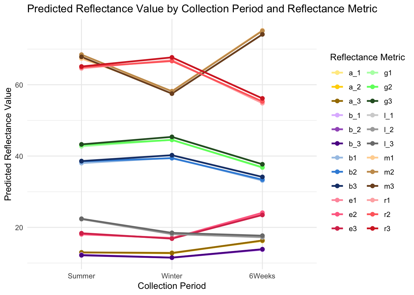
- Save the plot as a .pdf.
ggsave("output/predicted_reflectance_values.pdf", plot = p, width = 8, height = 6, device = "pdf")
sessionInfo()R version 4.4.1 (2024-06-14)
Platform: aarch64-apple-darwin20
Running under: macOS Sonoma 14.6.1
Matrix products: default
BLAS: /Library/Frameworks/R.framework/Versions/4.4-arm64/Resources/lib/libRblas.0.dylib
LAPACK: /Library/Frameworks/R.framework/Versions/4.4-arm64/Resources/lib/libRlapack.dylib; LAPACK version 3.12.0
locale:
[1] en_US.UTF-8/en_US.UTF-8/en_US.UTF-8/C/en_US.UTF-8/en_US.UTF-8
time zone: America/Detroit
tzcode source: internal
attached base packages:
[1] stats graphics grDevices utils datasets methods base
other attached packages:
[1] lme4_1.1-35.5 Matrix_1.7-0 viridis_0.6.5 viridisLite_0.4.2
[5] dplyr_1.1.4 ggeffects_1.7.1 ggplot2_3.5.1 ggstatsplot_0.12.4
loaded via a namespace (and not attached):
[1] gtable_0.3.5 xfun_0.47 bslib_0.8.0
[4] bayestestR_0.14.0 insight_0.20.5 lattice_0.22-6
[7] paletteer_1.6.0 vctrs_0.6.5 tools_4.4.1
[10] generics_0.1.3 datawizard_0.13.0 tibble_3.2.1
[13] fansi_1.0.6 highr_0.11 pkgconfig_2.0.3
[16] correlation_0.8.5 lifecycle_1.0.4 compiler_4.4.1
[19] farver_2.1.2 stringr_1.5.1 git2r_0.33.0
[22] textshaping_0.4.0 munsell_0.5.1 httpuv_1.6.15
[25] htmltools_0.5.8.1 sass_0.4.9 yaml_2.3.10
[28] crayon_1.5.3 nloptr_2.1.1 later_1.3.2
[31] pillar_1.9.0 jquerylib_0.1.4 whisker_0.4.1
[34] MASS_7.3-60.2 cachem_1.1.0 statsExpressions_1.6.0
[37] boot_1.3-30 nlme_3.1-164 tidyselect_1.2.1
[40] digest_0.6.37 mvtnorm_1.3-1 stringi_1.8.4
[43] purrr_1.0.2 rematch2_2.1.2 labeling_0.4.3
[46] forcats_1.0.0 splines_4.4.1 rprojroot_2.0.4
[49] fastmap_1.2.0 grid_4.4.1 colorspace_2.1-1
[52] cli_3.6.3 magrittr_2.0.3 patchwork_1.3.0
[55] utf8_1.2.4 withr_3.0.1 scales_1.3.0
[58] promises_1.3.0 estimability_1.5.1 rmarkdown_2.28
[61] emmeans_1.10.4 gridExtra_2.3 workflowr_1.7.1
[64] ragg_1.3.3 hms_1.1.3 coda_0.19-4.1
[67] evaluate_1.0.0 haven_2.5.4 knitr_1.48
[70] parameters_0.22.2 rlang_1.1.4 Rcpp_1.0.13
[73] zeallot_0.1.0 xtable_1.8-4 glue_1.7.0
[76] minqa_1.2.8 rstudioapi_0.16.0 jsonlite_1.8.9
[79] effectsize_0.8.9 R6_2.5.1 systemfonts_1.1.0
[82] fs_1.6.4