Last updated: 2025-11-18
Checks: 6 1
Knit directory: PAINT/
This reproducible R Markdown analysis was created with workflowr (version 1.7.1). The Checks tab describes the reproducibility checks that were applied when the results were created. The Past versions tab lists the development history.
The R Markdown file has unstaged changes. To know which version of
the R Markdown file created these results, you’ll want to first commit
it to the Git repo. If you’re still working on the analysis, you can
ignore this warning. When you’re finished, you can run
wflow_publish to commit the R Markdown file and build the
HTML.
Great job! The global environment was empty. Objects defined in the global environment can affect the analysis in your R Markdown file in unknown ways. For reproduciblity it’s best to always run the code in an empty environment.
The command set.seed(20251106) was run prior to running
the code in the R Markdown file. Setting a seed ensures that any results
that rely on randomness, e.g. subsampling or permutations, are
reproducible.
Great job! Recording the operating system, R version, and package versions is critical for reproducibility.
Nice! There were no cached chunks for this analysis, so you can be confident that you successfully produced the results during this run.
Great job! Using relative paths to the files within your workflowr project makes it easier to run your code on other machines.
Great! You are using Git for version control. Tracking code development and connecting the code version to the results is critical for reproducibility.
The results in this page were generated with repository version c8573bb. See the Past versions tab to see a history of the changes made to the R Markdown and HTML files.
Note that you need to be careful to ensure that all relevant files for
the analysis have been committed to Git prior to generating the results
(you can use wflow_publish or
wflow_git_commit). workflowr only checks the R Markdown
file, but you know if there are other scripts or data files that it
depends on. Below is the status of the Git repository when the results
were generated:
Ignored files:
    Ignored:    .RData
    Ignored:    .Rhistory
    Ignored:    .Rproj.user/
    Ignored:    data/neo_uvi.csv

Unstaged changes:
    Modified:   analysis/introduction.Rmd
Note that any generated files, e.g. HTML, png, CSS, etc., are not included in this status report because it is ok for generated content to have uncommitted changes.
These are the previous versions of the repository in which changes were
made to the R Markdown (analysis/introduction.Rmd) and HTML
(docs/introduction.html) files. If you’ve configured a
remote Git repository (see ?wflow_git_remote), click on the
hyperlinks in the table below to view the files as they were in that
past version.
| File | Version | Author | Date | Message |
|---|---|---|---|---|
| Rmd | c8573bb | Lily Heald | 2025-11-18 | add les Cottes |
| html | c8573bb | Lily Heald | 2025-11-18 | add les Cottes |
| Rmd | 0236dab | Lily Heald | 2025-11-13 | log transformed depth |
| html | 08dda7e | Lily Heald | 2025-11-13 | update depth plot |
| Rmd | 1bfb83f | Lily Heald | 2025-11-13 | update map, axes |
| Rmd | a1afed5 | Lily Heald | 2025-11-07 | update visibility |
| html | a1afed5 | Lily Heald | 2025-11-07 | update visibility |
| html | 735357b | Lily Heald | 2025-11-07 | Build site. |
| Rmd | 50940c0 | Lily Heald | 2025-11-07 | Update introduction.Rmd |
| Rmd | f1b70cb | Lily Heald | 2025-11-07 | add Hstadel depth |
| Rmd | 7beeddd | Lily Heald | 2025-11-07 | add depth figure |
| Rmd | 967f438 | Lily Heald | 2025-11-07 | update callout |
| html | 967f438 | Lily Heald | 2025-11-07 | update callout |
| html | cc7d134 | Lily Heald | 2025-11-06 | updated figures |
| Rmd | b2f5585 | Lily Heald | 2025-11-06 | Update introduction.Rmd |
| html | 13755f1 | Lily Heald | 2025-11-06 | workflowr |
| Rmd | 46a0913 | Lily Heald | 2025-11-06 | start workflowr |
world <- ne_countries(scale = "medium", returnclass = "sf")
uv_matrix <- as.matrix(read.csv("data/neo_uvi.csv", header = F))

lon <- seq(-179.75, 179.75, by = 0.5)
lat <- seq(89.75, -89.75, by = -0.5)

rownames(uv_matrix) <- lat
colnames(uv_matrix) <- lon

uv_df <- melt(uv_matrix, varnames = c("lat", "lon"), value.name = "UVIndex")

uv_df$lat <- as.numeric(as.character(uv_df$lat))
uv_df$lon <- as.numeric(as.character(uv_df$lon))
uv_raster <- rasterFromXYZ(uv_df[, c("lon", "lat", "UVIndex")], crs = "+proj=longlat +datum=WGS84")
world_sp <- as(world, "Spatial")
uv_land <- mask(uv_raster, world_sp)
uv_land_df <- as.data.frame(uv_land, xy = TRUE)
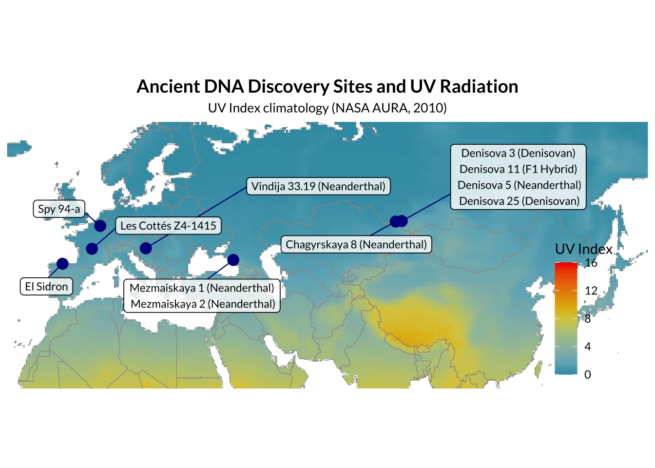
names(uv_land_df) <- c("lon", "lat", "UVIndex")sites <- data.frame(
name = c("Denisova","Chagyrskaya","Vindija", "Mezmaiskaya",
"El Sidron", "Spy","Les Cottés"),
samples = c("Denisova 3 (Denisovan)\nDenisova 11 (F1 Hybrid)\n Denisova 5 (Neanderthal)\n Denisova 25 (Denisovan)",
"Chagyrskaya 8 (Neanderthal)",
"Vindija 33.19 (Neanderthal)",
"Mezmaiskaya 1 (Neanderthal)\n Mezmaiskaya 2 (Neanderthal)",
"El Sidron",
"Spy 94-a",
"Les Cottés Z4-1415"),
lon = c(84.7, 83.1, 16.8, 40, -5.3, 4.7, 2.5), #E (+) W (-)
lat = c(51.4, 51.3, 46.3, 44.1, 43.4, 50.5, 46.2) #N (+) S (-)
)
sites_sf <- st_as_sf(sites, coords = c("lon","lat"), crs = 4326)Genome availability
wes_cols <- wes_palette("Zissou1", 100, type = "continuous")

ggplot() +
  geom_raster(data = uv_land_df, aes(x = lon, y = lat, fill = UVIndex)) +
  scale_fill_gradientn(colours = wes_cols, name = "UV Index", na.value = "white") +
  geom_sf(data = world, fill = NA, color = "grey60", size = 0.2) +
  geom_point(data = sites, aes(x = lon, y = lat),
             color = "#00008B", fill = "#00008B", shape = 21, size = 3, stroke = 1) +
  geom_label_repel(
    data = sites,
    aes(x = lon, y = lat, label = samples),
    box.padding = 0.7,
    point.padding = 0.3,
    segment.color = "#00008B",
    segment.size = 0.4,
    fill = alpha("white", 0.8),
    label.r = unit(0.2, "lines"),
    color = "black",
    size = 3,
    label.size = 0.3,
    family = "lato",
    min.segment.length = 0
  ) +
  coord_sf(expand = FALSE, xlim = c(-20, 150), ylim = c(20, 70)) +
  theme_minimal(base_family = "lato") +
  theme(
    legend.position = c(0.9, 0.3),
    legend.background = element_blank(),
    panel.grid = element_blank(),
    axis.text = element_blank(),
    axis.ticks = element_blank(),
    axis.title = element_blank(),
    plot.title = element_text(size = 14, face = "bold", hjust = 0.5),
    plot.subtitle = element_text(size = 10, hjust = 0.5)
  ) +
  labs(
    title = "Ancient DNA Discovery Sites and UV Radiation",
    subtitle = "UV Index climatology (NASA AURA, 2010)"
  )
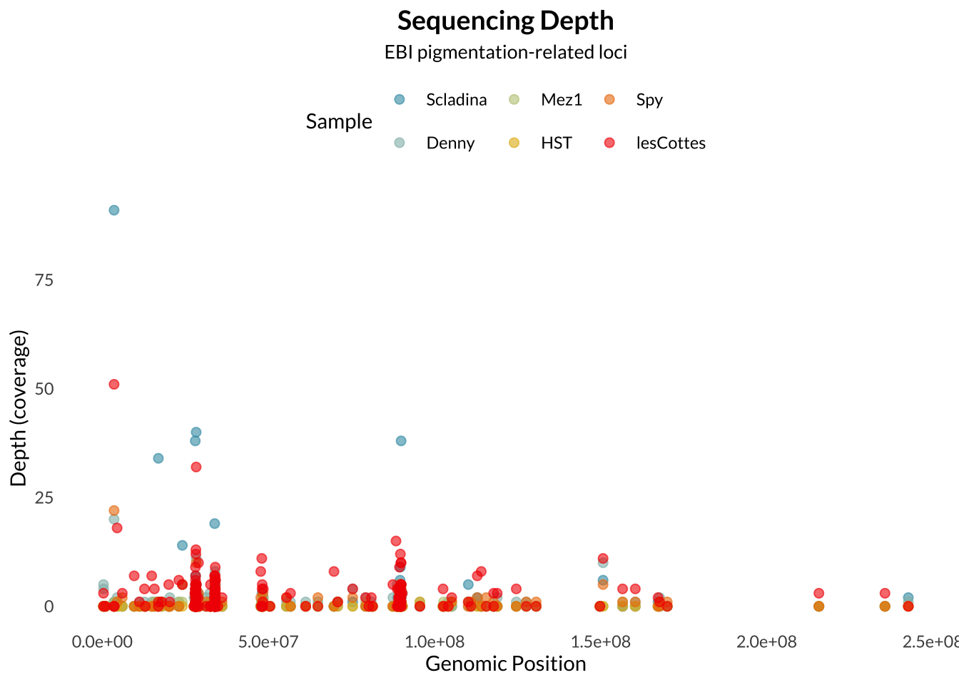
Sequencing coverage
wes_samples <- wes_palette("Zissou1", 6, type = "continuous")

ggplot(depth_all, aes(x = Position, y = Depth, color = Sample)) +
  geom_point(size = 2, alpha = 0.6) +
  scale_color_manual(values = wes_samples) +
  labs(
    title = "Sequencing Depth",
    subtitle = "EBI pigmentation-related loci",
    x = "Genomic Position",
    y = "Depth (coverage)",
    color = "Sample"
  ) +
  theme_bw(base_size = 14) +
  theme_minimal(base_family = "lato") +
  theme(
    legend.position = "top",
    legend.background = element_blank(),
    panel.grid = element_blank(),
    plot.title = element_text(size = 14, face = "bold", hjust = 0.5),
    plot.subtitle = element_text(size = 10, hjust = 0.5)
  )
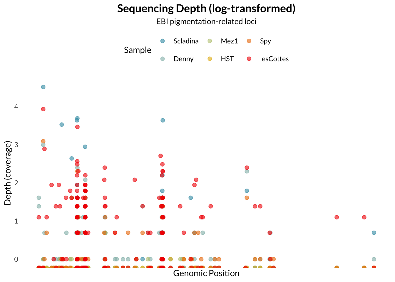
ggplot(depth_all, aes(x = Position, y = log(Depth), color = Sample)) +
  geom_point(size = 2, alpha = 0.6) +
  scale_color_manual(values = wes_samples) +
  labs(
    title = "Sequencing Depth (log-transformed)",
    subtitle = "EBI pigmentation-related loci",
    x = "Genomic Position",
    y = "Depth (coverage)",
    color = "Sample"
  ) +
  theme_bw(base_size = 14) +
  theme_minimal(base_family = "lato") +
  theme(
    legend.position = "top",
    legend.background = element_blank(),
    panel.grid = element_blank(),
    axis.text.x = element_blank(),
    plot.title = element_text(size = 14, face = "bold", hjust = 0.5),
    plot.subtitle = element_text(size = 10, hjust = 0.5)
  )
| Version | Author | Date |
|---|---|---|
| c8573bb | Lily Heald | 2025-11-18 |
sessionInfo()R version 4.4.2 (2024-10-31)
Platform: aarch64-apple-darwin20
Running under: macOS Monterey 12.5.1
Matrix products: default
BLAS: /Library/Frameworks/R.framework/Versions/4.4-arm64/Resources/lib/libRblas.0.dylib
LAPACK: /Library/Frameworks/R.framework/Versions/4.4-arm64/Resources/lib/libRlapack.dylib; LAPACK version 3.12.0
locale:
[1] en_US.UTF-8/en_US.UTF-8/en_US.UTF-8/C/en_US.UTF-8/en_US.UTF-8
time zone: America/Detroit
tzcode source: internal
attached base packages:
[1] stats graphics grDevices utils datasets methods base
other attached packages:
[1] wesanderson_0.3.7 showtext_0.9-7 showtextdb_3.0
[4] sysfonts_0.8.9 reshape2_1.4.4 lubridate_1.9.4
[7] forcats_1.0.0 stringr_1.5.2 dplyr_1.1.4
[10] purrr_1.0.4 readr_2.1.5 tidyr_1.3.1
[13] tibble_3.3.0 tidyverse_2.0.0 ggrepel_0.9.6
[16] viridis_0.6.5 viridisLite_0.4.2 ggspatial_1.1.10
[19] raster_3.6-32 sp_2.2-0 sf_1.0-21
[22] rnaturalearthdata_1.0.0 rnaturalearth_1.1.0 ggplot2_4.0.0
[25] workflowr_1.7.1
loaded via a namespace (and not attached):
[1] gtable_0.3.6 xfun_0.53 bslib_0.9.0 processx_3.8.6
[5] lattice_0.22-6 tzdb_0.5.0 callr_3.7.6 vctrs_0.6.5
[9] tools_4.4.2 ps_1.9.1 generics_0.1.4 curl_7.0.0
[13] proxy_0.4-27 pkgconfig_2.0.3 KernSmooth_2.23-26 RColorBrewer_1.1-3
[17] S7_0.2.0 lifecycle_1.0.4 compiler_4.4.2 farver_2.1.2
[21] git2r_0.35.0 terra_1.8-70 getPass_0.2-4 codetools_0.2-20
[25] httpuv_1.6.15 htmltools_0.5.8.1 class_7.3-23 sass_0.4.10
[29] yaml_2.3.10 later_1.4.4 pillar_1.11.1 jquerylib_0.1.4
[33] whisker_0.4.1 classInt_0.4-11 cachem_1.1.0 tidyselect_1.2.1
[37] digest_0.6.37 stringi_1.8.7 labeling_0.4.3 rprojroot_2.0.4
[41] fastmap_1.2.0 grid_4.4.2 cli_3.6.5 magrittr_2.0.4
[45] e1071_1.7-16 withr_3.0.2 scales_1.4.0 promises_1.3.3
[49] timechange_0.3.0 rmarkdown_2.29 httr_1.4.7 gridExtra_2.3
[53] hms_1.1.3 evaluate_1.0.5 knitr_1.50 rlang_1.1.6
[57] Rcpp_1.1.0 glue_1.8.0 DBI_1.2.3 rstudioapi_0.17.1
[61] jsonlite_2.0.0 plyr_1.8.9 R6_2.6.1 fs_1.6.6
[65] units_1.0-0