Fitness costs of SD chromosomes in Drosophila melanogaster
Luke Holman and Heidi Wong
2019-03-12
Last updated: 2019-03-12
Checks: 6 0
Knit directory: fitnessCostSD/
This reproducible R Markdown analysis was created with workflowr (version 1.2.0). The Report tab describes the reproducibility checks that were applied when the results were created. The Past versions tab lists the development history.
Great! Since the R Markdown file has been committed to the Git repository, you know the exact version of the code that produced these results.
Great job! The global environment was empty. Objects defined in the global environment can affect the analysis in your R Markdown file in unknown ways. For reproduciblity it’s best to always run the code in an empty environment.
The command set.seed(20190312) was run prior to running the code in the R Markdown file. Setting a seed ensures that any results that rely on randomness, e.g. subsampling or permutations, are reproducible.
Great job! Recording the operating system, R version, and package versions is critical for reproducibility.
Nice! There were no cached chunks for this analysis, so you can be confident that you successfully produced the results during this run.
Great! You are using Git for version control. Tracking code development and connecting the code version to the results is critical for reproducibility. The version displayed above was the version of the Git repository at the time these results were generated.
Note that you need to be careful to ensure that all relevant files for the analysis have been committed to Git prior to generating the results (you can use wflow_publish or wflow_git_commit). workflowr only checks the R Markdown file, but you know if there are other scripts or data files that it depends on. Below is the status of the Git repository when the results were generated:
Ignored files:
    Ignored:    .DS_Store
    Ignored:    .Rproj.user/
    Ignored:    data/.DS_Store
    Ignored:    docs/.DS_Store

Untracked files:
    Untracked:  data/SD_k tests_2018_04_05.xlsx
    Untracked:  data/clean_data/
    Untracked:  data/data collection sheet - follow up looking at sex ratio.xlsx
    Untracked:  data/data collection sheet from Heidi.xlsx
    Untracked:  data/messy_data/
    Untracked:  data/model_output/
    Untracked:  data/simulation_output.rds
    Untracked:  docs/figure/SD_costs_analysis.Rmd/
    Untracked:  docs/figure/evolutionary_simulation_SD.Rmd/
    Untracked:  figures/
    Untracked:  manuscript/
Note that any generated files, e.g. HTML, png, CSS, etc., are not included in this status report because it is ok for generated content to have uncommitted changes.
These are the previous versions of the R Markdown and HTML files. If you’ve configured a remote Git repository (see ?wflow_git_remote), click on the hyperlinks in the table below to view them.
| File | Version | Author | Date | Message |
|---|---|---|---|---|
| html | 6b03f9c | lukeholman | 2019-03-12 | Build site. |
| Rmd | 2bc25a0 | lukeholman | 2019-03-12 | Added main pages |
Set up for the analysis
Load R packages
packages <- c("dplyr", "brms", "ggplot2", "reshape2", "Cairo", "knitr", "pander", "lazerhawk",
              "grid", "gridExtra", "ggthemes", "readr", "tibble", "stringr")
shh <- suppressMessages(lapply(packages, library, character.only = TRUE, quietly = TRUE))
nCores <- 1

summarise_brms <- function(brmsfit){
  lazerhawk::brms_SummaryTable(brmsfit, astrology = TRUE) %>%
  mutate(Covariate = str_replace_all(Covariate, "SDM", "SD-"),
         Covariate = str_replace_all(Covariate, "SD-other", "SDMother")) %>%
  pander(split.cell = 40, split.table = Inf)
}
Load and clean the data
This section also saves a copy of the cleaned data in the directory data/cleaned_data. If you wish to re-use the data, I suggest you use these cleaned files; the factor and level names are more intuitive than in the original data sheets (however, the actual data are identical).
load_and_clean_data <- function(path){

   if(path == "data/messy_data/experiment2.csv"){

    expt2 <- read_csv(path) %>%
      mutate(prop_SD_females = female_SD / (female_SD + female_cyo),
             prop_SD_males = male_SD / (male_SD + male_cyo),
             prop_males = (male_SD + male_cyo) / (male_SD + male_cyo + female_SD + female_cyo),
             starting_number_focal_sex = num_embryos,
             SD_offspring = female_SD,
             CyO_offspring = female_cyo)

    expt2$starting_number_focal_sex[expt2$sex_of_embryos == "male"] <-
      expt2$starting_number_focal_sex[expt2$sex_of_embryos == "male"] -
      expt2$female_SD[expt2$sex_of_embryos == "male"] - expt2$female_cyo[expt2$sex_of_embryos == "male"]

    expt2$starting_number_focal_sex[expt2$sex_of_embryos == "female"] <-
      expt2$starting_number_focal_sex[expt2$sex_of_embryos == "female"] -
      expt2$male_SD[expt2$sex_of_embryos == "female"] - expt2$male_cyo[expt2$sex_of_embryos == "female"]

    expt2$SD_offspring[expt2$sex_of_embryos == "male"] <- expt2$male_SD[expt2$sex_of_embryos == "male"]
    expt2$CyO_offspring[expt2$sex_of_embryos == "male"] <- expt2$male_cyo[expt2$sex_of_embryos == "male"]

    expt2$starting_number_focal_sex[expt2$starting_number_focal_sex < expt2$SD_focal_sex] <-
      expt2$SD_focal_sex[expt2$starting_number_focal_sex < expt2$SD_focal_sex]

    expt2$Dead_offspring <- expt2$starting_number_focal_sex - expt2$SD_offspring - expt2$CyO_offspring
    expt2$Dead_offspring[expt2$Dead_offspring < 0] <- 0

    expt2$starting_number_focal_sex <- with(expt2, SD_offspring + CyO_offspring + Dead_offspring)

    expt2 <- expt2 %>%
      select(block, SD_parent, sex_of_embryos, SD, starting_number_focal_sex, SD_offspring, CyO_offspring, Dead_offspring) %>%
      mutate(vial = 1:n(),
             SD_embryos = "to be estimated",
             CyO_embryos = "to be estimated",
             block = as.numeric(as.factor(block))) %>%
      filter(!(SD %in% c("w1118", "LHm")))
    write_csv(expt2, path = str_replace(path, "messy", "clean"))
    return(expt2)
  }

  # For experiment 1....
  dat <- read_csv(path) %>%
    mutate(block = as.character(block),
           copies_of_SD = substr(genotype, 2, 2),
           parent_with_SD = substr(genotype, 1, 1),
           parent_with_SD = replace(parent_with_SD,
                                    parent_with_SD == "M", "Mother"),
           parent_with_SD = replace(parent_with_SD,
                                    parent_with_SD == "P", "Father"),
           parent_with_SD = replace(parent_with_SD,
                                    parent_with_SD == "A", "Both parents"),
           parent_with_SD = replace(parent_with_SD,
                                    parent_with_SD == "N", "Neither parent"),
           parent_with_SD =  factor(parent_with_SD,
                                    levels = c("Neither parent",
                                               "Father", "Mother",
                                               "Both parents")),
           SD = paste("SD-", SD, sep = ""),
           SD = replace(SD, SD == "SD-N", "No SD chromosome"),

           MotherHasSD = ifelse(parent_with_SD != "Father", 1, 0),
           FatherHasSD = ifelse(parent_with_SD != "Mother", 1, 0),
           MotherHasSD = replace(MotherHasSD, SD == "No SD chromosome", 0),
           FatherHasSD = replace(FatherHasSD, SD == "No SD chromosome", 0),
           SD_from_mum = ifelse(MotherHasSD==1 & copies_of_SD=="1", "Yes", "No"),
           SD_from_mum = replace(SD_from_mum, FatherHasSD==1 & MotherHasSD==1 & copies_of_SD=="2", "Yes"),
           SD_from_dad = ifelse(FatherHasSD == 1 & copies_of_SD == "1", "Yes", "No"),
           SD_from_dad = replace(SD_from_dad, FatherHasSD==1 & MotherHasSD==1 & copies_of_SD=="2", "Yes"),
           mum_genotype = relevel(as.factor(ifelse(MotherHasSD==1, SD, "wild_type")), ref = "wild_type"),
           dad_genotype = relevel(as.factor(ifelse(FatherHasSD==1, SD, "wild_type")), ref = "wild_type"))

  if(path == "data/messy_data/male_fitness.csv"){
    dat <- dat %>%
      mutate(focal.male.fitness = focal_daughters + focal_sons,
             rival.male.fitness = rival_daughters + rival_sons,
             total = focal.male.fitness + rival.male.fitness,
             vial = 1:n())
  }

  if(path == "data/messy_data/larval_fitness.csv"){

    # Note that for 'Mother has SD' crosses (Cross 2), the 'initial_number' of larvae is the maximum possible.
    # The real initial number of non-recombinants is probably a bit lower, since the survival rate of the recombinants is probably not 100%
    # This means the survival rate in Cross 2 is an under-estimate of the true survival rate.
    # For SD-5, it is a very slight underestimate, since SD-5 does not recombine much.
    # For the other two SDs, it is a larger underestimate.

    dat <- dat %>%
      mutate(surviving_females = nonrecombinant_females,
             surviving_males = nonrecombinant_males,
             survivors = nonrecombinant_females + nonrecombinant_males,
             initial_number = number_larvae_in_vial - recombinant_females - recombinant_males,
             number_died = initial_number - survivors,
             larval_density = as.numeric(scale(number_larvae_in_vial)), # mean-centre the larval density covariate
             vial = 1:n(),
             total = survivors + number_died) %>%
      select(-number_larvae_in_vial, -nonrecombinant_females, -nonrecombinant_males, -recombinant_females, -recombinant_males)

    # We never put more than 100 larvae in one vial, so for cases where the initial number was 200, it was 2 vials of 100 each, etc.
    dat$larval_density[dat$larval_density > 100] <- 100

    # For Cross 1, where both parents have SD, we cannot discriminate larvae with 0 or 1 copies of SD
    # (until they become adults and develop eyes)
    dat$copies_of_SD[dat$genotype == "A0+A1"] <- "0 or 1"
  }

  if(path == "data/messy_data/female_fitness.csv"){
    dat$vial <- 1:nrow(dat)
  }

  # 'genotype' variable is a composite of SD genotype and parental origin, used during data collection. Not needed for analysis
  dat <- dat %>% select(-genotype)

  # save the clean data
  write_csv(dat, path = str_replace(path, "messy", "clean"))
  dat
}

larvae  <- load_and_clean_data("data/messy_data/larval_fitness.csv")
males   <- load_and_clean_data("data/messy_data/male_fitness.csv")
females <- load_and_clean_data("data/messy_data/female_fitness.csv")
expt2   <- load_and_clean_data("data/messy_data/experiment2.csv")
Summary statistics for the four response variables
Larval survival data
Table S1: Number and percentage of L1 larvae surviving to adulthood for each SD genotype and cross type.
larvae %>%
  group_by(SD, copies_of_SD, parent_with_SD) %>%
  summarise(number_larvae_counted = sum(survivors + number_died),
            number_of_survivors = sum(survivors),
            percent_surviving = 100 * (number_of_survivors / number_larvae_counted)) %>%
    mutate(percent_surviving = format(round(percent_surviving, 1), nsmall = 1)) %>%
as.data.frame() %>% pander(split.cell = 40, split.table = Inf)| SD | copies_of_SD | parent_with_SD | number_larvae_counted | number_of_survivors | percent_surviving |
|---|---|---|---|---|---|
| No SD chromosome | 0 | Neither parent | 600 | 495 | 82.5 |
| SD-5 | 0 | Father | 113 | 89 | 78.8 |
| SD-5 | 0 | Mother | 459 | 408 | 88.9 |
| SD-5 | 0 or 1 | Both parents | 700 | 520 | 74.3 |
| SD-5 | 1 | Father | 563 | 412 | 73.2 |
| SD-5 | 1 | Mother | 494 | 415 | 84.0 |
| SD-5 | 2 | Both parents | 40 | 0 | 0.0 |
| SD-72 | 0 | Father | 287 | 226 | 78.7 |
| SD-72 | 0 | Mother | 396 | 333 | 84.1 |
| SD-72 | 0 or 1 | Both parents | 700 | 542 | 77.4 |
| SD-72 | 1 | Father | 600 | 477 | 79.5 |
| SD-72 | 1 | Mother | 423 | 342 | 80.9 |
| SD-72 | 2 | Both parents | 600 | 0 | 0.0 |
| SD-Mad | 0 | Father | 296 | 239 | 80.7 |
| SD-Mad | 0 | Mother | 371 | 279 | 75.2 |
| SD-Mad | 0 or 1 | Both parents | 700 | 558 | 79.7 |
| SD-Mad | 1 | Father | 600 | 462 | 77.0 |
| SD-Mad | 1 | Mother | 436 | 320 | 73.4 |
| SD-Mad | 2 | Both parents | 585 | 413 | 70.6 |
Adult sex ratio
Table S2: Number and percentage of male and female adults emerging from the juvenile fitness assay vials.
larvae %>% group_by(SD, copies_of_SD, parent_with_SD) %>%
  summarise(n.males = sum(surviving_males),
            n.females = sum(surviving_females),
            n.total = sum(survivors),
            percent.male = format(round(100 * sum(surviving_males) / n.total, 1), nsmall = 1)) %>%
as.data.frame() %>% pander(split.cell = 40, split.table = Inf)| SD | copies_of_SD | parent_with_SD | n.males | n.females | n.total | percent.male |
|---|---|---|---|---|---|---|
| No SD chromosome | 0 | Neither parent | 267 | 228 | 495 | 53.9 |
| SD-5 | 0 | Father | 48 | 41 | 89 | 53.9 |
| SD-5 | 0 | Mother | 206 | 202 | 408 | 50.5 |
| SD-5 | 0 or 1 | Both parents | 239 | 281 | 520 | 46.0 |
| SD-5 | 1 | Father | 196 | 216 | 412 | 47.6 |
| SD-5 | 1 | Mother | 193 | 222 | 415 | 46.5 |
| SD-5 | 2 | Both parents | 0 | 0 | 0 | NaN |
| SD-72 | 0 | Father | 105 | 121 | 226 | 46.5 |
| SD-72 | 0 | Mother | 169 | 164 | 333 | 50.8 |
| SD-72 | 0 or 1 | Both parents | 272 | 270 | 542 | 50.2 |
| SD-72 | 1 | Father | 233 | 244 | 477 | 48.8 |
| SD-72 | 1 | Mother | 186 | 156 | 342 | 54.4 |
| SD-72 | 2 | Both parents | 0 | 0 | 0 | NaN |
| SD-Mad | 0 | Father | 102 | 137 | 239 | 42.7 |
| SD-Mad | 0 | Mother | 145 | 134 | 279 | 52.0 |
| SD-Mad | 0 or 1 | Both parents | 253 | 305 | 558 | 45.3 |
| SD-Mad | 1 | Father | 190 | 272 | 462 | 41.1 |
| SD-Mad | 1 | Mother | 184 | 136 | 320 | 57.5 |
| SD-Mad | 2 | Both parents | 209 | 204 | 413 | 50.6 |
Male fitness data
Table S3: Average relative fitness of adult males for each SD genotype and cross type, expressed as the average proportion of offspring sired. The last two columns give the sample size in terms of number of vials (each of which contained 5 focal males), and number of males.
SE <- function(x) sd(x) / sqrt(length(x))
males %>%
  group_by(SD, copies_of_SD, parent_with_SD) %>%
  summarise(average_relative_fitness = mean(focal.male.fitness / (focal.male.fitness + rival.male.fitness)),
            SE = SE(focal.male.fitness / (focal.male.fitness + rival.male.fitness)),
            number_of_vials = n(),
            number_of_males = number_of_vials * 5) %>%
  mutate(average_relative_fitness = format(round(average_relative_fitness, 2), nsmall = 2),
         SE = format(round(SE, 3), nsmall = 3)) %>%
as.data.frame() %>% pander(split.cell = 40, split.table = Inf)| SD | copies_of_SD | parent_with_SD | average_relative_fitness | SE | number_of_vials | number_of_males |
|---|---|---|---|---|---|---|
| No SD chromosome | 0 | Neither parent | 0.79 | 0.040 | 13 | 65 |
| SD-5 | 0 | Father | 0.68 | 0.147 | 5 | 25 |
| SD-5 | 0 | Mother | 0.82 | 0.045 | 17 | 85 |
| SD-5 | 0 | Both parents | 0.59 | NA | 1 | 5 |
| SD-5 | 1 | Father | 0.14 | 0.055 | 18 | 90 |
| SD-5 | 1 | Mother | 0.32 | 0.072 | 12 | 60 |
| SD-5 | 1 | Both parents | 0.39 | 0.074 | 13 | 65 |
| SD-72 | 0 | Father | 0.88 | 0.027 | 16 | 80 |
| SD-72 | 0 | Mother | 0.77 | 0.054 | 13 | 65 |
| SD-72 | 0 | Both parents | 0.79 | NA | 1 | 5 |
| SD-72 | 1 | Father | 0.76 | 0.045 | 18 | 90 |
| SD-72 | 1 | Mother | 0.80 | 0.039 | 17 | 85 |
| SD-72 | 1 | Both parents | 0.67 | 0.051 | 19 | 95 |
| SD-Mad | 0 | Father | 0.75 | 0.055 | 14 | 70 |
| SD-Mad | 0 | Mother | 0.75 | 0.069 | 11 | 55 |
| SD-Mad | 0 | Both parents | 0.82 | 0.078 | 5 | 25 |
| SD-Mad | 1 | Father | 0.87 | 0.028 | 18 | 90 |
| SD-Mad | 1 | Mother | 0.81 | 0.037 | 17 | 85 |
| SD-Mad | 1 | Both parents | 0.75 | 0.053 | 18 | 90 |
| SD-Mad | 2 | Both parents | 0.19 | 0.072 | 14 | 70 |
Female fitness data
Table S4: Average fecundity of adult females for each SD genotype and cross type. The last two columns give the sample size in terms of number of oviposition vials (each of which contained up to 5 focal females), and number of males.
females %>%
  mutate(larvae_per_female = larvae_produced / number_of_laying_females) %>%
  group_by(SD, copies_of_SD, parent_with_SD) %>%
  summarise(average_fecundity = mean(larvae_per_female),
            SE = SE(larvae_per_female),
            number_of_vials = n(),
            number_of_females = sum(number_of_laying_females)) %>%
  mutate(average_fecundity = format(round(average_fecundity, 2), nsmall = 2),
         SE = format(round(SE, 3), nsmall = 3)) %>%
as.data.frame() %>% pander(split.cell = 40, split.table = Inf)| SD | copies_of_SD | parent_with_SD | average_fecundity | SE | number_of_vials | number_of_females |
|---|---|---|---|---|---|---|
| No SD chromosome | 0 | Neither parent | 26.55 | 3.874 | 10 | 48 |
| SD-5 | 0 | Father | 25.06 | 8.127 | 6 | 28 |
| SD-5 | 0 | Mother | 41.13 | 3.700 | 15 | 71 |
| SD-5 | 0 | Both parents | 24.95 | 3.767 | 5 | 22 |
| SD-5 | 1 | Father | 28.88 | 3.337 | 12 | 55 |
| SD-5 | 1 | Mother | 29.74 | 3.118 | 16 | 69 |
| SD-5 | 1 | Both parents | 26.83 | 2.583 | 15 | 67 |
| SD-72 | 0 | Father | 32.68 | 3.258 | 14 | 65 |
| SD-72 | 0 | Mother | 35.10 | 3.023 | 15 | 68 |
| SD-72 | 0 | Both parents | 22.53 | 6.671 | 3 | 15 |
| SD-72 | 1 | Father | 33.97 | 2.743 | 16 | 77 |
| SD-72 | 1 | Mother | 41.90 | 3.792 | 14 | 68 |
| SD-72 | 1 | Both parents | 31.85 | 2.885 | 15 | 73 |
| SD-Mad | 0 | Father | 28.25 | 3.769 | 16 | 79 |
| SD-Mad | 0 | Mother | 44.71 | 3.723 | 13 | 65 |
| SD-Mad | 0 | Both parents | 16.50 | 1.762 | 3 | 14 |
| SD-Mad | 1 | Father | 36.85 | 3.968 | 16 | 77 |
| SD-Mad | 1 | Mother | 40.58 | 4.602 | 14 | 64 |
| SD-Mad | 1 | Both parents | 34.88 | 3.478 | 16 | 76 |
| SD-Mad | 2 | Both parents | 11.26 | 1.631 | 17 | 83 |
Experiment 2 larval survival data
Table S5: Number and percentage of L1 larvae surviving to adulthood in Experiment 2, for each SD genotype, cross type, and offspring sex.
set.seed(1)
expt2 %>%
  rename(parent_with_SD = SD_parent, offspring_sex = sex_of_embryos) %>%
  mutate(SD_embryos = SD_offspring + rbinom(n(), Dead_offspring, 0.5),
         CyO_embryos = starting_number_focal_sex - SD_embryos,
         parent_with_SD = ifelse(parent_with_SD == "dad", "Father", "Mother"),
         offspring_sex = ifelse(offspring_sex == "female", "Female", "Male")) %>%
  group_by(SD, parent_with_SD, offspring_sex) %>%
  summarise(percent_surviving_SD_larvae = mean(100 * SD_offspring / SD_embryos),
            percent_surviving_CyO_larvae = mean(100 * CyO_offspring / CyO_embryos),
            n_larvae_counted = sum(starting_number_focal_sex),
            n_crosses = n()) %>%
  mutate(percent_surviving_SD_larvae = format(round(percent_surviving_SD_larvae, 1), nsmall = 1),
         percent_surviving_CyO_larvae = format(round(percent_surviving_CyO_larvae, 1), nsmall = 1)) %>%
pander(split.cell = 40, split.table = Inf)| SD | parent_with_SD | offspring_sex | percent_surviving_SD_larvae | percent_surviving_CyO_larvae | n_larvae_counted | n_crosses |
|---|---|---|---|---|---|---|
| SD-5 | Father | Female | 81.0 | 86.0 | 763 | 16 |
| SD-5 | Father | Male | 79.1 | 79.4 | 727 | 17 |
| SD-5 | Mother | Female | 76.3 | 82.1 | 871 | 18 |
| SD-5 | Mother | Male | 68.2 | 69.9 | 972 | 20 |
| SD-72 | Father | Female | 86.3 | 85.4 | 744 | 16 |
| SD-72 | Father | Male | 83.7 | 77.9 | 615 | 15 |
| SD-72 | Mother | Female | 89.5 | 88.1 | 1123 | 23 |
| SD-72 | Mother | Male | 78.7 | 77.6 | 1186 | 24 |
| SD-Mad | Father | Female | 86.2 | 85.5 | 457 | 10 |
| SD-Mad | Father | Male | 86.2 | 84.1 | 480 | 11 |
| SD-Mad | Mother | Female | 84.4 | 85.2 | 942 | 20 |
| SD-Mad | Mother | Male | 82.1 | 78.6 | 1010 | 21 |
Analysis of L1 larva-to-adult survival
Run a Bayesian binomial generalised linear mixed model
if(!file.exists("data/model_output/larvae_brms.rds")){

  larvae_brms <-  brm(survivors | trials(total) ~ larval_density + SD * copies_of_SD * parent_with_SD + (1 | vial),
                      family = binomial,
                      data = larvae,
                      iter = 4000, chains = 4, cores = nCores,
                      control = list(adapt_delta = 0.99, max_treedepth = 15),
                      prior = prior(normal(0, 5), class = "b"))

  saveRDS(larvae_brms, "data/model_output/larvae_brms.rds")
} else larvae_brms <- readRDS("data/model_output/larvae_brms.rds")
Check a diagnostic plot of the model
This plot shows the frequency distribution of the original data (black line), along with predicted data that were computed using 10 random samples from the posterior of the model parameters. The posterior predicted values closely match the originals, suggesting that the model is approximating the data reasonably well.
pp_check(larvae_brms)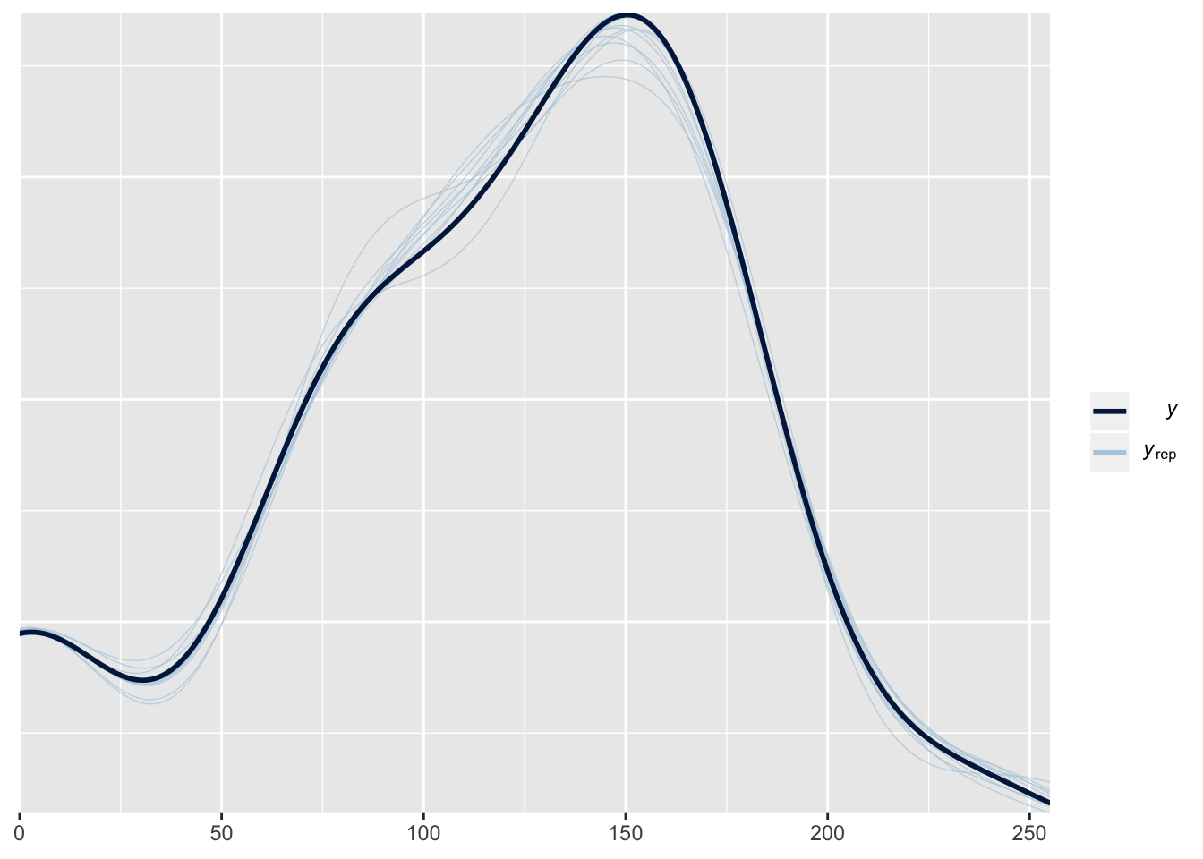
| Version | Author | Date |
|---|---|---|
| 6b03f9c | lukeholman | 2019-03-12 |
Inspect the model summary
This summary shows the median, error, and 95% CIs for the posterior for all the fixed effects. This table is difficult to interpret and not very informative, but is presented here for completeness.
summarise_brms(larvae_brms)| Covariate | Estimate | Est.Error | l-95% CI | u-95% CI | Notable |
|---|---|---|---|---|---|
| Intercept | 1.64 | 0.34 | 0.97 | 2.32 | * |
| larval_density | -0.04 | 0.17 | -0.37 | 0.31 | |
| SDSD-5 | -0.57 | 3.18 | -6.69 | 5.57 | |
| SDSD-72 | -0.79 | 3.18 | -7.07 | 5.43 | |
| SDSD-Mad | 0.19 | 3.17 | -6.16 | 6.49 | |
| copies_of_SD0or1 | 0.89 | 4.29 | -7.55 | 9.18 | |
| copies_of_SD1 | -0.07 | 3.55 | -7.08 | 6.88 | |
| copies_of_SD2 | -2.56 | 4.31 | -11.00 | 5.91 | |
| parent_with_SDFather | 0.04 | 3.06 | -5.90 | 5.98 | |
| parent_with_SDMother | 0.35 | 3.04 | -5.64 | 6.33 | |
| parent_with_SDBothparents | -1.75 | 4.10 | -9.63 | 6.33 | |
| SDSD-5:copies_of_SD0or1 | 0.78 | 4.29 | -7.69 | 9.14 | |
| SDSD-72:copies_of_SD0or1 | 1.04 | 4.40 | -7.63 | 9.81 | |
| SDSD-Mad:copies_of_SD0or1 | -0.89 | 4.31 | -9.41 | 7.68 | |
| SDSD-5:copies_of_SD1 | -0.16 | 3.55 | -7.05 | 6.74 | |
| SDSD-72:copies_of_SD1 | 0.08 | 3.53 | -6.79 | 6.97 | |
| SDSD-Mad:copies_of_SD1 | -0.03 | 3.54 | -6.97 | 6.90 | |
| SDSD-5:copies_of_SD2 | -2.16 | 4.53 | -11.22 | 6.71 | |
| SDSD-72:copies_of_SD2 | -2.78 | 4.65 | -11.86 | 6.34 | |
| SDSD-Mad:copies_of_SD2 | 2.35 | 4.41 | -6.37 | 11.11 | |
| SDSD-5:parent_with_SDFather | 0.03 | 3.42 | -6.59 | 6.91 | |
| SDSD-72:parent_with_SDFather | 0.37 | 3.46 | -6.53 | 7.19 | |
| SDSD-Mad:parent_with_SDFather | -0.45 | 3.45 | -7.31 | 6.26 | |
| SDSD-5:parent_with_SDMother | 0.73 | 3.42 | -5.87 | 7.58 | |
| SDSD-72:parent_with_SDMother | 0.51 | 3.32 | -6.05 | 7.12 | |
| SDSD-Mad:parent_with_SDMother | -0.89 | 3.37 | -7.41 | 5.86 | |
| SDSD-5:parent_with_SDBothparents | -1.38 | 4.16 | -9.58 | 6.70 | |
| SDSD-72:parent_with_SDBothparents | -1.65 | 4.26 | -9.96 | 6.89 | |
| SDSD-Mad:parent_with_SDBothparents | 1.37 | 4.13 | -6.77 | 9.69 | |
| copies_of_SD0or1:parent_with_SDFather | -0.01 | 5.11 | -10.16 | 10.02 | |
| copies_of_SD1:parent_with_SDFather | 0.03 | 3.54 | -6.90 | 6.94 | |
| copies_of_SD2:parent_with_SDFather | 0.11 | 4.99 | -9.60 | 9.91 | |
| copies_of_SD0or1:parent_with_SDMother | -0.04 | 4.91 | -9.60 | 9.63 | |
| copies_of_SD1:parent_with_SDMother | -0.13 | 3.63 | -7.24 | 7.09 | |
| copies_of_SD2:parent_with_SDMother | 0.06 | 5.06 | -9.76 | 9.81 | |
| copies_of_SD0or1:parent_with_SDBothparents | 0.89 | 4.23 | -7.16 | 9.22 | |
| copies_of_SD1:parent_with_SDBothparents | 0.08 | 4.90 | -9.61 | 9.82 | |
| copies_of_SD2:parent_with_SDBothparents | -2.68 | 4.37 | -11.18 | 5.82 | |
| SDSD-5:copies_of_SD0or1:parent_with_SDFather | 0.01 | 4.93 | -9.76 | 9.63 | |
| SDSD-72:copies_of_SD0or1:parent_with_SDFather | -0.03 | 5.09 | -10.10 | 10.02 | |
| SDSD-Mad:copies_of_SD0or1:parent_with_SDFather | 0.00 | 5.08 | -9.93 | 9.91 | |
| SDSD-5:copies_of_SD1:parent_with_SDFather | 0.06 | 3.53 | -6.84 | 6.90 | |
| SDSD-72:copies_of_SD1:parent_with_SDFather | 0.11 | 3.55 | -6.86 | 7.07 | |
| SDSD-Mad:copies_of_SD1:parent_with_SDFather | -0.11 | 3.57 | -7.17 | 6.86 | |
| SDSD-5:copies_of_SD2:parent_with_SDFather | 0.09 | 5.06 | -9.60 | 9.95 | |
| SDSD-72:copies_of_SD2:parent_with_SDFather | 0.04 | 4.94 | -9.58 | 9.60 | |
| SDSD-Mad:copies_of_SD2:parent_with_SDFather | -0.01 | 4.96 | -9.76 | 9.88 | |
| SDSD-5:copies_of_SD0or1:parent_with_SDMother | 0.03 | 5.09 | -9.86 | 10.08 | |
| SDSD-72:copies_of_SD0or1:parent_with_SDMother | 0.02 | 4.96 | -9.67 | 9.71 | |
| SDSD-Mad:copies_of_SD0or1:parent_with_SDMother | -0.03 | 4.97 | -9.89 | 9.64 | |
| SDSD-5:copies_of_SD1:parent_with_SDMother | -0.14 | 3.60 | -7.19 | 6.93 | |
| SDSD-72:copies_of_SD1:parent_with_SDMother | -0.10 | 3.64 | -7.21 | 7.11 | |
| SDSD-Mad:copies_of_SD1:parent_with_SDMother | 0.12 | 3.58 | -6.92 | 7.18 | |
| SDSD-5:copies_of_SD2:parent_with_SDMother | 0.01 | 4.86 | -9.39 | 9.50 | |
| SDSD-72:copies_of_SD2:parent_with_SDMother | -0.02 | 5.06 | -9.93 | 9.87 | |
| SDSD-Mad:copies_of_SD2:parent_with_SDMother | 0.04 | 5.02 | -9.64 | 9.90 | |
| SDSD-5:copies_of_SD0or1:parent_with_SDBothparents | 0.76 | 4.26 | -7.48 | 8.94 | |
| SDSD-72:copies_of_SD0or1:parent_with_SDBothparents | 0.99 | 4.41 | -7.54 | 9.71 | |
| SDSD-Mad:copies_of_SD0or1:parent_with_SDBothparents | -0.85 | 4.30 | -9.30 | 7.38 | |
| SDSD-5:copies_of_SD1:parent_with_SDBothparents | -0.05 | 4.89 | -9.48 | 9.44 | |
| SDSD-72:copies_of_SD1:parent_with_SDBothparents | 0.09 | 5.12 | -9.96 | 10.17 | |
| SDSD-Mad:copies_of_SD1:parent_with_SDBothparents | 0.00 | 4.97 | -9.69 | 9.78 | |
| SDSD-5:copies_of_SD2:parent_with_SDBothparents | -2.17 | 4.58 | -11.16 | 6.77 | |
| SDSD-72:copies_of_SD2:parent_with_SDBothparents | -2.80 | 4.54 | -11.78 | 5.99 | |
| SDSD-Mad:copies_of_SD2:parent_with_SDBothparents | 2.32 | 4.36 | -6.35 | 10.75 |
Hypothesis testing
Table S6: The results of hypothesis tests computed using the model of larval survival in Experiment 1. Each row gives the posterior estimate of a difference in means, such that the estimate is positive if mean 1 is larger than mean 2, and negative otherwise (expressed in % larval survival). The mean 1 and mean 2 columns list the parent which had SD (mother, father, or both), followed by the number of SD alleles present in the offspring (0, 1 or 2). The Posterior probability column gives the probability that the mean with the smaller point estimate is actually larger than the other mean, analagously to a one-tailed p-value. The Evidence ratio (ER) column gives the ratio of evidence, such that ER = 5 means that it is 5 times more likely that the mean with the smaller point estimate really is the smaller one. Asterisks highlight rows where the posterior probability is less than 0.05.
# Function to compute posterior difference in means, with the posterior_probability of the smaller mean actually being the larger one (plus the larger evidence ratio, e.g. ER = 10 means it's 10x more likely the smaller mean really is smaller not larger, ER=1 means it's equally likely the smaller one is actually larger)
compare <- function(mean1, mean2){
  difference <- mean1 - mean2
  prob_less <- hypothesis(data.frame(x = difference), "x < 0")$hypothesis
  prob_more <- hypothesis(data.frame(x = difference), "x > 0")$hypothesis
  hypothesis(data.frame(x = difference), "x = 0")$hypothesis %>%
    mutate(Posterior_probability = min(c(prob_less$Post.Prob, prob_more$Post.Prob)),
           Evidence_ratio = max(c(prob_less$Evid.Ratio, prob_more$Evid.Ratio)))
}

hypothesis_tests <- function(model, dat, SR = FALSE, divisor = NULL){

  SDs <- c("SD-5", "SD-72", "SD-Mad")

  new <- dat %>%
    select(SD, copies_of_SD, MotherHasSD, FatherHasSD, SD_from_mum,
           SD_from_dad, mum_genotype, dad_genotype, parent_with_SD) %>%
    distinct() %>%
    arrange(SD, copies_of_SD, MotherHasSD, FatherHasSD, SD_from_mum,
            SD_from_dad, mum_genotype, dad_genotype) %>%
    mutate(total = 100,
           number_of_laying_females = 5,
           larval_density = 0,
           copies_of_SD = as.character(copies_of_SD),
           i = 1:n(),
           parent = ifelse(FatherHasSD == 1, "B", "M"),
           parent = replace(parent, MotherHasSD == 0, "F"))


  SD5 <- new %>% filter(SD == "SD-5")
  SD72 <- new %>% filter(SD == "SD-72")
  SDMad <- new %>% filter(SD == "SD-Mad")

  pred <- fitted(model, re_formula = NA,
                 newdata = new,
                 summary = FALSE)

  if(!is.null(divisor)) pred <- pred / divisor

  control_0SD_neither <- pred[, new %>% filter(SD == "No SD chromosome") %>% pull(i)]

  SD5_0SD_mother <- pred[, SD5 %>% filter(copies_of_SD == "0" & parent == "M") %>% pull(i)]
  SD5_1SD_mother <- pred[, SD5 %>% filter(copies_of_SD == "1" & parent == "M") %>% pull(i)]
  SD5_0SD_father <- pred[, SD5 %>% filter(copies_of_SD == "0" & parent == "F") %>% pull(i)]
  SD5_1SD_father <- pred[, SD5 %>% filter(copies_of_SD == "1" & parent == "F") %>% pull(i)]

  SD72_0SD_mother <- pred[, SD72 %>% filter(copies_of_SD == "0" & parent == "M") %>% pull(i)]
  SD72_1SD_mother <- pred[, SD72 %>% filter(copies_of_SD == "1" & parent == "M") %>% pull(i)]
  SD72_0SD_father <- pred[, SD72 %>% filter(copies_of_SD == "0" & parent == "F") %>% pull(i)]
  SD72_1SD_father <- pred[, SD72 %>% filter(copies_of_SD == "1" & parent == "F") %>% pull(i)]

  SDMad_0SD_mother <- pred[, SDMad %>% filter(copies_of_SD == "0" & parent == "M") %>% pull(i)]
  SDMad_1SD_mother <- pred[, SDMad %>% filter(copies_of_SD == "1" & parent == "M") %>% pull(i)]
  SDMad_0SD_father <- pred[, SDMad %>% filter(copies_of_SD == "0" & parent == "F") %>% pull(i)]
  SDMad_1SD_father <- pred[, SDMad %>% filter(copies_of_SD == "1" & parent == "F") %>% pull(i)]

  SDMad_1SD_both <- pred[, SDMad %>% filter(copies_of_SD %in% c("0 or 1", "1") & parent == "B") %>% pull(i)]
  SDMad_2 <- pred[, SDMad %>% filter(copies_of_SD == "2") %>% pull(i)]

  # For larvae data only, we also have observations of SD-5 and SD-Mad homozygotes
  if(sum(new$copies_of_SD == "2") > 1){
    SD5_1SD_both  <- pred[, SD5  %>% filter(copies_of_SD %in% c("0 or 1", "1") & parent == "B") %>% pull(i)]
    SD72_1SD_both <- pred[, SD72 %>% filter(copies_of_SD %in% c("0 or 1", "1") & parent == "B") %>% pull(i)]
    SD5_2  <- pred[, SD5  %>% filter(copies_of_SD == "2") %>% pull(i)]
    SD72_2 <- pred[, SD72 %>% filter(copies_of_SD == "2") %>% pull(i)]

    two_compare <- data.frame(
      SD = SDs,
      Mean_1 = rep(paste("Both parents,", ifelse("0 or 1" %in% SD5$copies_of_SD, "0 or 1", "1")), 3),
      Mean_2 = rep("Both parents, 2", 3),
      rbind(
        compare(SD5_1SD_both, SD5_2),
        compare(SD72_1SD_both, SD72_2),
        compare(SDMad_1SD_both, SDMad_2)
      )
    )

  } else { # for non-larva data
    two_compare <- data.frame(SD = "SD-Mad",
                              Mean_1 = "Both parents, 1",
                              Mean_2 = "Both parents, 2",
                              compare(SDMad_1SD_both, SDMad_2)) # CONTROLS HERE
  }

  if("0 or 1" %in% new$copies_of_SD){
    SD5_0or1   <- pred[, SD5 %>% filter(copies_of_SD == "0 or 1") %>% pull(i)]
    SD72_0or1  <- pred[, SD72 %>% filter(copies_of_SD == "0 or 1") %>% pull(i)]
    SDMad_0or1 <- pred[, SDMad %>% filter(copies_of_SD == "0 or 1") %>% pull(i)]
  }

  rbind(
    data.frame(
      SD = rep(SDs, 6),
      Mean_1 = c(rep("Neither, 0", 6), rep("Mother, 0", 3), rep("Mother, 1", 3), rep("Mother, 0", 3), rep("Father, 0", 3)),
      Mean_2 = c(rep("Father, 0", 3), rep("Mother, 0", 3),
                 rep("Father, 0", 3), rep("Father, 1", 3), rep("Mother, 1", 3), rep("Father, 1", 3)),
      rbind(

        compare(control_0SD_neither, SD5_0SD_father), # controls vs 0 SD individuals
        compare(control_0SD_neither, SD72_0SD_father),
        compare(control_0SD_neither, SDMad_0SD_father),
        compare(control_0SD_neither, SD5_0SD_mother),
        compare(control_0SD_neither, SD72_0SD_mother),
        compare(control_0SD_neither, SDMad_0SD_mother),

        compare(SD5_0SD_mother, SD5_0SD_father), # parental effects on 0 SD individuals
        compare(SD72_0SD_mother, SD72_0SD_father),
        compare(SDMad_0SD_mother, SDMad_0SD_father),

        compare(SD5_1SD_mother, SD5_1SD_father), # parental effects on 1 SD individuals
        compare(SD72_1SD_mother, SD72_1SD_father),
        compare(SDMad_1SD_mother, SDMad_1SD_father),

        compare(SD5_0SD_mother, SD5_1SD_mother), # effect of inheriting SD, from the mother
        compare(SD72_0SD_mother, SD72_1SD_mother),
        compare(SDMad_0SD_mother, SDMad_1SD_mother),

        compare(SD5_0SD_father, SD5_1SD_father), # effect of inheriting SD, from the father
        compare(SD72_0SD_father, SD72_1SD_father),
        compare(SDMad_0SD_father, SDMad_1SD_father)

      )),
    two_compare) %>%
    select(-Hypothesis, -Evid.Ratio, -Post.Prob, -Star) %>%
    mutate(Notable = ifelse(Posterior_probability < 0.05, "*", ""))
}

clean_table <- function(tabl){
  cols <- c("Trait", "SD", "Comparison", "Difference", "Error", "Posterior_probability")
  if(!("Trait" %in% names(tabl))){
    cols <- cols[cols != "Trait"]
  }

  tabl <- mutate(tabl,
                 Estimate = format(round(Estimate, 1), nsmall = 1),
                 Est.Error = format(round(Est.Error, 1), nsmall = 1),
                 CI.Lower = format(round(CI.Lower, 1), nsmall = 1),
                 CI.Upper = format(round(CI.Upper, 1), nsmall = 1),
                 Evidence_ratio = format(round(Evidence_ratio, 1), nsmall = 1),
                 Difference = paste(Estimate, " (", CI.Lower, " to ", CI.Upper, ")", sep = ""),
                 Comparison = paste(Mean_1, "-", Mean_2),
                 Error = Est.Error) %>%
    select(!! cols)
  names(tabl) <- str_replace_all(names(tabl), "_", " ")
  tabl
}

tests1 <- hypothesis_tests(larvae_brms, larvae)
tests1 %>% clean_table() %>% pander(split.cell = 40, split.table = Inf)| SD | Comparison | Difference | Error | Posterior probability |
|---|---|---|---|---|
| SD-5 | Neither, 0 - Father, 0 | 8.9 (-11.6 to 34.9) | 11.8 | 0.2254 |
| SD-72 | Neither, 0 - Father, 0 | 6.0 (-10.5 to 24.3) | 8.9 | 0.2464 |
| SD-Mad | Neither, 0 - Father, 0 | 3.5 (-12.5 to 21.0) | 8.4 | 0.3415 |
| SD-5 | Neither, 0 - Mother, 0 | -5.8 (-18.1 to 5.3) | 5.9 | 0.1557 |
| SD-72 | Neither, 0 - Mother, 0 | -0.9 (-14.0 to 12.1) | 6.6 | 0.4435 |
| SD-Mad | Neither, 0 - Mother, 0 | 5.4 ( -9.3 to 20.0) | 7.3 | 0.2181 |
| SD-5 | Mother, 0 - Father, 0 | 14.7 ( -2.8 to 39.3) | 10.7 | 0.0575 |
| SD-72 | Mother, 0 - Father, 0 | 6.9 ( -9.6 to 25.0) | 8.8 | 0.2145 |
| SD-Mad | Mother, 0 - Father, 0 | -1.9 (-18.1 to 15.9) | 8.6 | 0.3991 |
| SD-5 | Mother, 1 - Father, 1 | 10.6 ( -4.4 to 26.4) | 7.8 | 0.07975 |
| SD-72 | Mother, 1 - Father, 1 | 1.2 (-13.1 to 15.4) | 7.2 | 0.429 |
| SD-Mad | Mother, 1 - Father, 1 | -1.0 (-17.9 to 15.2) | 8.4 | 0.4487 |
| SD-5 | Mother, 0 - Mother, 1 | 5.6 ( -5.2 to 17.4) | 5.7 | 0.156 |
| SD-72 | Mother, 0 - Mother, 1 | 3.0 (-10.2 to 16.9) | 6.8 | 0.326 |
| SD-Mad | Mother, 0 - Mother, 1 | 1.9 (-14.4 to 19.4) | 8.6 | 0.4131 |
| SD-5 | Father, 0 - Father, 1 | 1.6 (-25.5 to 23.4) | 12.5 | 0.4146 |
| SD-72 | Father, 0 - Father, 1 | -2.7 (-21.5 to 15.1) | 9.3 | 0.3935 |
| SD-Mad | Father, 0 - Father, 1 | 2.8 (-16.7 to 20.4) | 9.2 | 0.3656 |
| SD-5 | Both parents, 0 or 1 - Both parents, 2 | 77.1 ( 62.2 to 87.8) | 6.5 | 0 |
| SD-72 | Both parents, 0 or 1 - Both parents, 2 | 77.5 ( 63.6 to 87.8) | 6.1 | 0 |
| SD-Mad | Both parents, 0 or 1 - Both parents, 2 | 10.6 ( -6.7 to 27.7) | 8.7 | 0.1046 |
Analysis of adult sex ratio
Run a Bayesian binomial generalised linear mixed model
SR_data <- larvae %>% filter(survivors > 0) %>%
  mutate(Males = surviving_males,
         total = surviving_males + surviving_females)

if(!file.exists("data/model_output/SR_brms.rds")){
  SR_brms <-  brm(Males | trials(total) ~ SD * copies_of_SD * parent_with_SD + (1 | vial),
                  family = binomial,
                  data = SR_data, iter = 4000, chains = 4, cores = nCores,
                  control = list(adapt_delta = 0.99, max_treedepth = 15),
                  prior = prior(normal(0, 5), class = "b"))

  saveRDS(SR_brms, "data/model_output/SR_brms.rds")
} else SR_brms <- readRDS("data/model_output/SR_brms.rds")
Check a diagnostic plot of the model
This plot shows the frequency distribution of the original data (black line), along with predicted data that were computed using 10 random samples from the posterior of the model parameters. The posterior predicted values closely match the originals, suggesting that the model is approximating the data reasonably well.
pp_check(SR_brms)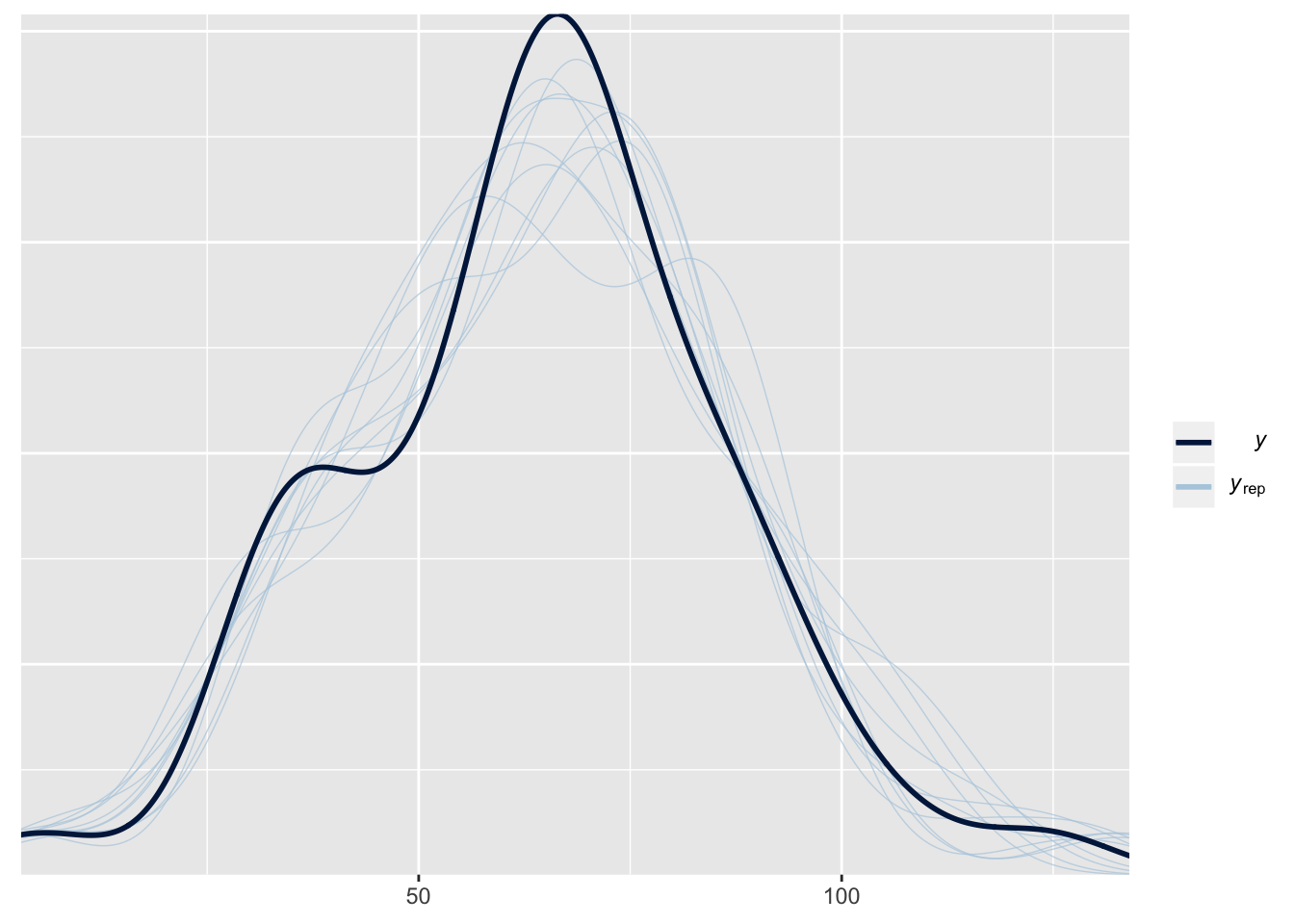
| Version | Author | Date |
|---|---|---|
| 6b03f9c | lukeholman | 2019-03-12 |
Inspect the model summary
This summary shows the median, error, and 95% CIs for the posterior for all the fixed effects. This table is difficult to interpret and not very informative, but is presented here for completeness.
summarise_brms(SR_brms)| Covariate | Estimate | Est.Error | l-95% CI | u-95% CI | Notable |
|---|---|---|---|---|---|
| Intercept | 0.15 | 0.16 | -0.16 | 0.46 | |
| SDSD-5 | 0.06 | 3.20 | -6.28 | 6.28 | |
| SDSD-72 | -0.08 | 3.19 | -6.29 | 6.31 | |
| SDSD-Mad | -0.13 | 3.15 | -6.34 | 5.91 | |
| copies_of_SD0or1 | -0.10 | 4.36 | -8.53 | 8.54 | |
| copies_of_SD1 | 0.03 | 3.55 | -6.99 | 6.99 | |
| copies_of_SD2 | -0.01 | 4.54 | -9.04 | 8.98 | |
| parent_with_SDFather | -0.12 | 3.05 | -6.15 | 5.89 | |
| parent_with_SDMother | -0.01 | 3.07 | -5.99 | 5.92 | |
| parent_with_SDBothparents | -0.03 | 4.15 | -8.19 | 8.13 | |
| SDSD-5:copies_of_SD0or1 | -0.11 | 4.31 | -8.51 | 8.49 | |
| SDSD-72:copies_of_SD0or1 | 0.04 | 4.35 | -8.57 | 8.45 | |
| SDSD-Mad:copies_of_SD0or1 | -0.07 | 4.27 | -8.43 | 8.10 | |
| SDSD-5:copies_of_SD1 | -0.17 | 3.61 | -7.23 | 6.96 | |
| SDSD-72:copies_of_SD1 | 0.05 | 3.53 | -6.84 | 6.96 | |
| SDSD-Mad:copies_of_SD1 | 0.03 | 3.53 | -6.85 | 6.93 | |
| SDSD-5:copies_of_SD2 | 0.01 | 5.00 | -9.76 | 9.78 | |
| SDSD-72:copies_of_SD2 | 0.02 | 5.02 | -9.82 | 9.99 | |
| SDSD-Mad:copies_of_SD2 | 0.01 | 4.47 | -8.64 | 8.77 | |
| SDSD-5:parent_with_SDFather | 0.07 | 3.42 | -6.61 | 6.85 | |
| SDSD-72:parent_with_SDFather | -0.08 | 3.37 | -6.74 | 6.44 | |
| SDSD-Mad:parent_with_SDFather | -0.20 | 3.41 | -6.80 | 6.50 | |
| SDSD-5:parent_with_SDMother | -0.15 | 3.48 | -6.98 | 6.78 | |
| SDSD-72:parent_with_SDMother | -0.03 | 3.41 | -6.73 | 6.52 | |
| SDSD-Mad:parent_with_SDMother | 0.11 | 3.42 | -6.61 | 6.87 | |
| SDSD-5:parent_with_SDBothparents | -0.03 | 4.31 | -8.53 | 8.36 | |
| SDSD-72:parent_with_SDBothparents | -0.01 | 4.40 | -8.72 | 8.59 | |
| SDSD-Mad:parent_with_SDBothparents | -0.01 | 4.17 | -8.43 | 8.09 | |
| copies_of_SD0or1:parent_with_SDFather | -0.01 | 4.91 | -9.76 | 9.72 | |
| copies_of_SD1:parent_with_SDFather | -0.02 | 3.50 | -7.03 | 6.85 | |
| copies_of_SD2:parent_with_SDFather | 0.06 | 4.97 | -9.73 | 9.93 | |
| copies_of_SD0or1:parent_with_SDMother | 0.02 | 5.00 | -9.91 | 9.73 | |
| copies_of_SD1:parent_with_SDMother | 0.06 | 3.49 | -6.85 | 6.98 | |
| copies_of_SD2:parent_with_SDMother | 0.01 | 5.08 | -9.92 | 10.00 | |
| copies_of_SD0or1:parent_with_SDBothparents | -0.05 | 4.32 | -8.58 | 8.30 | |
| copies_of_SD1:parent_with_SDBothparents | 0.03 | 4.98 | -9.69 | 9.86 | |
| copies_of_SD2:parent_with_SDBothparents | 0.05 | 4.48 | -8.89 | 8.87 | |
| SDSD-5:copies_of_SD0or1:parent_with_SDFather | -0.04 | 4.95 | -9.71 | 9.82 | |
| SDSD-72:copies_of_SD0or1:parent_with_SDFather | 0.03 | 5.11 | -9.90 | 10.00 | |
| SDSD-Mad:copies_of_SD0or1:parent_with_SDFather | 0.03 | 4.98 | -9.82 | 9.78 | |
| SDSD-5:copies_of_SD1:parent_with_SDFather | -0.09 | 3.50 | -6.93 | 6.85 | |
| SDSD-72:copies_of_SD1:parent_with_SDFather | 0.04 | 3.54 | -6.93 | 6.90 | |
| SDSD-Mad:copies_of_SD1:parent_with_SDFather | -0.09 | 3.54 | -7.00 | 6.89 | |
| SDSD-5:copies_of_SD2:parent_with_SDFather | 0.04 | 5.01 | -9.56 | 9.79 | |
| SDSD-72:copies_of_SD2:parent_with_SDFather | 0.00 | 4.84 | -9.52 | 9.55 | |
| SDSD-Mad:copies_of_SD2:parent_with_SDFather | -0.04 | 5.05 | -9.75 | 10.02 | |
| SDSD-5:copies_of_SD0or1:parent_with_SDMother | -0.09 | 5.05 | -10.00 | 9.75 | |
| SDSD-72:copies_of_SD0or1:parent_with_SDMother | -0.01 | 4.92 | -9.78 | 9.66 | |
| SDSD-Mad:copies_of_SD0or1:parent_with_SDMother | 0.01 | 4.97 | -9.72 | 9.53 | |
| SDSD-5:copies_of_SD1:parent_with_SDMother | -0.12 | 3.57 | -7.11 | 6.90 | |
| SDSD-72:copies_of_SD1:parent_with_SDMother | 0.02 | 3.44 | -6.68 | 6.75 | |
| SDSD-Mad:copies_of_SD1:parent_with_SDMother | 0.16 | 3.50 | -6.79 | 7.13 | |
| SDSD-5:copies_of_SD2:parent_with_SDMother | 0.05 | 4.94 | -9.42 | 9.67 | |
| SDSD-72:copies_of_SD2:parent_with_SDMother | -0.02 | 5.01 | -9.83 | 9.61 | |
| SDSD-Mad:copies_of_SD2:parent_with_SDMother | 0.02 | 4.95 | -9.76 | 9.99 | |
| SDSD-5:copies_of_SD0or1:parent_with_SDBothparents | -0.05 | 4.37 | -8.45 | 8.44 | |
| SDSD-72:copies_of_SD0or1:parent_with_SDBothparents | 0.08 | 4.45 | -8.39 | 8.82 | |
| SDSD-Mad:copies_of_SD0or1:parent_with_SDBothparents | 0.05 | 4.25 | -8.36 | 8.33 | |
| SDSD-5:copies_of_SD1:parent_with_SDBothparents | 0.05 | 4.97 | -9.73 | 9.99 | |
| SDSD-72:copies_of_SD1:parent_with_SDBothparents | -0.03 | 5.04 | -10.04 | 9.77 | |
| SDSD-Mad:copies_of_SD1:parent_with_SDBothparents | 0.01 | 4.95 | -9.71 | 9.58 | |
| SDSD-5:copies_of_SD2:parent_with_SDBothparents | 0.00 | 5.06 | -9.77 | 10.07 | |
| SDSD-72:copies_of_SD2:parent_with_SDBothparents | -0.04 | 4.93 | -9.73 | 9.63 | |
| SDSD-Mad:copies_of_SD2:parent_with_SDBothparents | -0.01 | 4.54 | -8.94 | 8.88 |
Hypothesis testing
Table S7: The results of hypothesis tests computed using the model of adult sex ratio in Experiment 1. Each row gives the posterior estimate of a difference in means, such that the estimate is positive if mean 1 is larger than mean 2, and negative otherwise (expressed in % males). The mean 1 and mean 2 columns list the parent which had SD (mother, father, or both), followed by the number of SD alleles present in the offspring (0, 1 or 2). The Posterior probability column gives the probability that the mean with the smaller point estimate is actually larger than the other mean, analagously to a one-tailed p-value. The Evidence ratio (ER) column gives the ratio of evidence, such that ER = 5 means that it is 5 times more likely that the mean with the smaller point estimate really is the smaller one. Asterisks highlight rows where the posterior probability is less than 0.05.
tests2 <- hypothesis_tests(SR_brms, SR_data)
tests2 %>% clean_table() %>% pander(split.cell = 40, split.table = Inf)| SD | Comparison | Difference | Error | Posterior probability |
|---|---|---|---|---|
| SD-5 | Neither, 0 - Father, 0 | -0.3 (-15.9 to 15.7) | 8.1 | 0.482 |
| SD-72 | Neither, 0 - Father, 0 | 7.2 ( -4.9 to 19.1) | 6.1 | 0.1136 |
| SD-Mad | Neither, 0 - Father, 0 | 11.1 ( -0.8 to 23.0) | 6.0 | 0.03387 |
| SD-5 | Neither, 0 - Mother, 0 | 2.5 ( -9.0 to 13.7) | 5.7 | 0.323 |
| SD-72 | Neither, 0 - Mother, 0 | 3.2 ( -7.9 to 14.5) | 5.7 | 0.2835 |
| SD-Mad | Neither, 0 - Mother, 0 | 0.9 (-11.0 to 12.4) | 5.9 | 0.437 |
| SD-5 | Mother, 0 - Father, 0 | -2.8 (-18.4 to 13.4) | 8.1 | 0.3619 |
| SD-72 | Mother, 0 - Father, 0 | 4.0 ( -8.5 to 16.1) | 6.3 | 0.2602 |
| SD-Mad | Mother, 0 - Father, 0 | 10.2 ( -2.7 to 22.6) | 6.3 | 0.05613 |
| SD-5 | Mother, 1 - Father, 1 | -1.5 (-13.0 to 9.9) | 5.7 | 0.3913 |
| SD-72 | Mother, 1 - Father, 1 | 5.6 ( -5.8 to 17.0) | 5.7 | 0.1593 |
| SD-Mad | Mother, 1 - Father, 1 | 18.3 ( 7.1 to 29.7) | 5.7 | 0.001375 |
| SD-5 | Mother, 0 - Mother, 1 | 5.1 ( -6.2 to 16.6) | 5.8 | 0.1869 |
| SD-72 | Mother, 0 - Mother, 1 | -3.9 (-15.7 to 7.9) | 6.0 | 0.2506 |
| SD-Mad | Mother, 0 - Mother, 1 | -6.7 (-18.6 to 5.0) | 6.0 | 0.128 |
| SD-5 | Father, 0 - Father, 1 | 6.3 ( -9.9 to 22.4) | 8.1 | 0.2083 |
| SD-72 | Father, 0 - Father, 1 | -2.3 (-13.8 to 9.5) | 6.0 | 0.343 |
| SD-Mad | Father, 0 - Father, 1 | 1.4 (-10.2 to 13.2) | 5.9 | 0.4101 |
| SD-Mad | Both parents, 1 - Both parents, 2 | -5.2 (-16.1 to 5.9) | 5.5 | 0.1635 |
Analysis of adult female fitness
Run a Bayesian negative binomial generalised linear mixed model
if(!file.exists("data/model_output/female_brms.rds")){
  female_brms <-  brm(larvae_produced ~ number_of_laying_females + SD * copies_of_SD * parent_with_SD,
                    family = negbinomial,
                    data = females, iter = 4000, chains = 4, cores = nCores,
                    control = list(adapt_delta = 0.99, max_treedepth = 15),
                    prior = prior(normal(0, 5), class = "b"))

  saveRDS(female_brms, "data/model_output/female_brms.rds")
} else female_brms <- readRDS("data/model_output/female_brms.rds")
Check a diagnostic plot of the model
This plot shows the frequency distribution of the original data (black line), along with predicted data that were computed using 10 random samples from the posterior of the model parameters. The posterior predicted values closely match the originals, suggesting that the model is approximating the data reasonably well.
pp_check(female_brms)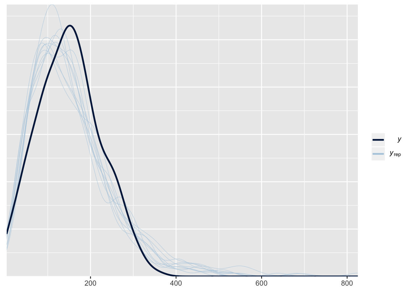
| Version | Author | Date |
|---|---|---|
| 6b03f9c | lukeholman | 2019-03-12 |
Inspect the model summary
This summary shows the median, error, and 95% CIs for the posterior for all the fixed effects. This table is difficult to interpret and not very informative, but is presented here for completeness.
summarise_brms(female_brms)| Covariate | Estimate | Est.Error | l-95% CI | u-95% CI | Notable |
|---|---|---|---|---|---|
| Intercept | 3.97 | 0.34 | 3.32 | 4.64 | * |
| number_of_laying_females | 0.18 | 0.06 | 0.06 | 0.30 | * |
| SDSD-5 | 0.04 | 3.00 | -5.88 | 5.84 | |
| SDSD-72 | 0.07 | 2.96 | -5.62 | 5.75 | |
| SDSD-Mad | 0.09 | 3.04 | -5.93 | 6.02 | |
| copies_of_SD1 | 0.06 | 3.39 | -6.59 | 6.60 | |
| copies_of_SD2 | -0.08 | 4.31 | -8.50 | 8.48 | |
| parent_with_SDFather | 0.01 | 3.02 | -5.86 | 5.94 | |
| parent_with_SDMother | 0.20 | 3.03 | -5.77 | 6.12 | |
| parent_with_SDBothparents | -0.19 | 3.02 | -6.19 | 5.73 | |
| SDSD-5:copies_of_SD1 | -0.03 | 3.27 | -6.46 | 6.38 | |
| SDSD-72:copies_of_SD1 | 0.09 | 3.26 | -6.28 | 6.39 | |
| SDSD-Mad:copies_of_SD1 | 0.17 | 3.31 | -6.19 | 6.65 | |
| SDSD-5:copies_of_SD2 | 0.03 | 4.88 | -9.70 | 9.71 | |
| SDSD-72:copies_of_SD2 | 0.00 | 5.00 | -9.67 | 9.74 | |
| SDSD-Mad:copies_of_SD2 | -0.12 | 4.43 | -8.81 | 8.62 | |
| SDSD-5:parent_with_SDFather | -0.13 | 3.28 | -6.55 | 6.27 | |
| SDSD-72:parent_with_SDFather | 0.12 | 3.28 | -6.38 | 6.59 | |
| SDSD-Mad:parent_with_SDFather | -0.03 | 3.28 | -6.39 | 6.44 | |
| SDSD-5:parent_with_SDMother | 0.19 | 3.26 | -6.31 | 6.46 | |
| SDSD-72:parent_with_SDMother | -0.01 | 3.25 | -6.41 | 6.43 | |
| SDSD-Mad:parent_with_SDMother | 0.24 | 3.35 | -6.43 | 6.69 | |
| SDSD-5:parent_with_SDBothparents | 0.08 | 3.20 | -6.25 | 6.23 | |
| SDSD-72:parent_with_SDBothparents | -0.02 | 3.32 | -6.56 | 6.49 | |
| SDSD-Mad:parent_with_SDBothparents | -0.35 | 3.34 | -6.82 | 6.28 | |
| copies_of_SD1:parent_with_SDFather | -0.01 | 3.36 | -6.55 | 6.45 | |
| copies_of_SD2:parent_with_SDFather | -0.06 | 5.06 | -9.93 | 9.53 | |
| copies_of_SD1:parent_with_SDMother | -0.18 | 3.34 | -6.74 | 6.51 | |
| copies_of_SD2:parent_with_SDMother | -0.01 | 4.99 | -9.67 | 9.78 | |
| copies_of_SD1:parent_with_SDBothparents | 0.14 | 3.29 | -6.31 | 6.50 | |
| copies_of_SD2:parent_with_SDBothparents | -0.01 | 4.30 | -8.55 | 8.40 | |
| SDSD-5:copies_of_SD1:parent_with_SDFather | 0.13 | 3.31 | -6.35 | 6.54 | |
| SDSD-72:copies_of_SD1:parent_with_SDFather | -0.10 | 3.22 | -6.42 | 6.30 | |
| SDSD-Mad:copies_of_SD1:parent_with_SDFather | 0.04 | 3.38 | -6.58 | 6.66 | |
| SDSD-5:copies_of_SD2:parent_with_SDFather | -0.02 | 5.06 | -10.04 | 9.88 | |
| SDSD-72:copies_of_SD2:parent_with_SDFather | 0.03 | 5.05 | -9.86 | 9.96 | |
| SDSD-Mad:copies_of_SD2:parent_with_SDFather | 0.02 | 4.94 | -9.61 | 9.85 | |
| SDSD-5:copies_of_SD1:parent_with_SDMother | -0.22 | 3.31 | -6.65 | 6.15 | |
| SDSD-72:copies_of_SD1:parent_with_SDMother | 0.22 | 3.33 | -6.21 | 6.79 | |
| SDSD-Mad:copies_of_SD1:parent_with_SDMother | -0.18 | 3.38 | -6.81 | 6.37 | |
| SDSD-5:copies_of_SD2:parent_with_SDMother | 0.02 | 4.98 | -9.75 | 10.09 | |
| SDSD-72:copies_of_SD2:parent_with_SDMother | 0.00 | 4.94 | -9.60 | 9.69 | |
| SDSD-Mad:copies_of_SD2:parent_with_SDMother | 0.01 | 5.02 | -9.79 | 9.80 | |
| SDSD-5:copies_of_SD1:parent_with_SDBothparents | -0.12 | 3.25 | -6.41 | 6.20 | |
| SDSD-72:copies_of_SD1:parent_with_SDBothparents | 0.02 | 3.32 | -6.32 | 6.66 | |
| SDSD-Mad:copies_of_SD1:parent_with_SDBothparents | 0.34 | 3.33 | -6.18 | 6.87 | |
| SDSD-5:copies_of_SD2:parent_with_SDBothparents | 0.02 | 5.00 | -9.75 | 9.82 | |
| SDSD-72:copies_of_SD2:parent_with_SDBothparents | -0.05 | 4.96 | -9.70 | 9.57 | |
| SDSD-Mad:copies_of_SD2:parent_with_SDBothparents | -0.20 | 4.42 | -8.76 | 8.64 |
Hypothesis testing
Table S8: The results of hypothesis tests computed using the model of female fitness in Experiment 1. Each row gives the posterior estimate of a difference in means, such that the estimate is positive if mean 1 is larger than mean 2, and negative otherwise (expressed as the number of offspring produced). The mean 1 and mean 2 columns list the parent which had SD (mother, father, or both), followed by the number of SD alleles present in the offspring (0, 1 or 2). The Posterior probability column gives the probability that the mean with the smaller point estimate is actually larger than the other mean, analagously to a one-tailed p-value. The Evidence ratio (ER) column gives the ratio of evidence, such that ER = 5 means that it is 5 times more likely that the mean with the smaller point estimate really is the smaller one. Asterisks highlight rows where the posterior probability is less than 0.05.
tests3 <- hypothesis_tests(female_brms, females, divisor = 5)
tests3 %>% clean_table() %>% pander(split.cell = 40, split.table = Inf)| SD | Comparison | Difference | Error | Posterior probability |
|---|---|---|---|---|
| SD-5 | Neither, 0 - Father, 0 | 1.9 (-12.3 to 14.7) | 6.9 | 0.3684 |
| SD-72 | Neither, 0 - Father, 0 | -5.8 (-18.5 to 6.5) | 6.2 | 0.1609 |
| SD-Mad | Neither, 0 - Father, 0 | -1.7 (-12.7 to 9.9) | 5.8 | 0.3711 |
| SD-5 | Neither, 0 - Mother, 0 | -14.4 (-28.6 to -0.4) | 7.0 | 0.02187 |
| SD-72 | Neither, 0 - Mother, 0 | -7.9 (-20.5 to 4.5) | 6.4 | 0.1049 |
| SD-Mad | Neither, 0 - Mother, 0 | -18.7 (-34.7 to -3.8) | 7.8 | 0.005875 |
| SD-5 | Mother, 0 - Father, 0 | 16.4 ( 1.0 to 31.0) | 7.6 | 0.01862 |
| SD-72 | Mother, 0 - Father, 0 | 2.0 (-10.9 to 14.7) | 6.4 | 0.3709 |
| SD-Mad | Mother, 0 - Father, 0 | 17.0 ( 3.2 to 32.6) | 7.5 | 0.008625 |
| SD-5 | Mother, 1 - Father, 1 | -0.1 (-11.5 to 10.8) | 5.7 | 0.4999 |
| SD-72 | Mother, 1 - Father, 1 | 8.2 ( -5.5 to 22.8) | 7.2 | 0.1254 |
| SD-Mad | Mother, 1 - Father, 1 | 3.4 (-10.5 to 17.7) | 7.2 | 0.3214 |
| SD-5 | Mother, 0 - Mother, 1 | 12.5 ( -0.2 to 26.1) | 6.6 | 0.02687 |
| SD-72 | Mother, 0 - Mother, 1 | -7.5 (-22.5 to 6.9) | 7.4 | 0.1456 |
| SD-Mad | Mother, 0 - Mother, 1 | 5.4 (-10.9 to 22.3) | 8.5 | 0.2546 |
| SD-5 | Father, 0 - Father, 1 | -3.9 (-16.9 to 10.1) | 6.8 | 0.2641 |
| SD-72 | Father, 0 - Father, 1 | -1.4 (-13.9 to 11.4) | 6.3 | 0.412 |
| SD-Mad | Father, 0 - Father, 1 | -8.2 (-20.4 to 3.4) | 6.0 | 0.07975 |
| SD-Mad | Both parents, 1 - Both parents, 2 | 23.4 ( 15.0 to 33.1) | 4.6 | 0 |
Analysis of adult male fitness
Run a Bayesian binomial generalised linear mixed model
if(!file.exists("data/model_output/male_brms.rds")){
  male_brms <-  brm(focal.male.fitness | trials(total) ~ SD * copies_of_SD * parent_with_SD + (1 | vial),
                    family = binomial,
                    data = males, iter = 4000, chains = 4, cores = nCores,
                    control = list(adapt_delta = 0.99, max_treedepth = 15),
                    prior = prior(normal(0, 5), class = "b"))

  saveRDS(male_brms, "data/model_output/male_brms.rds")
} else male_brms <- readRDS("data/model_output/male_brms.rds")
Check a diagnostic plot of the model
This plot shows the frequency distribution of the original data (black line), along with predicted data that were computed using 10 random samples from the posterior of the model parameters. The posterior predicted values closely match the originals, suggesting that the model is approximating the data reasonably well.
pp_check(male_brms)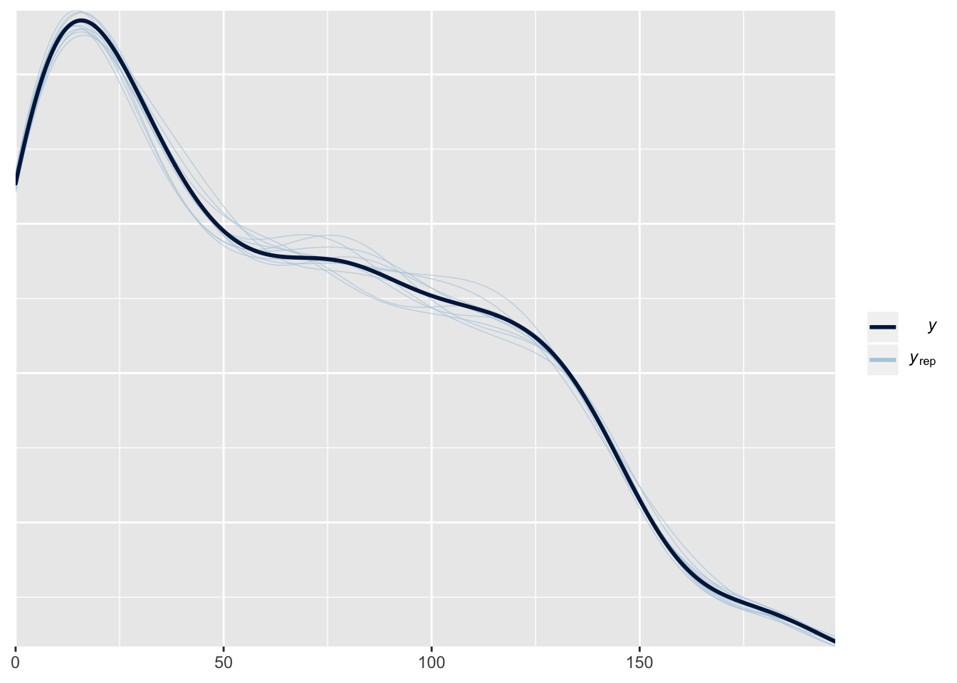
| Version | Author | Date |
|---|---|---|
| 6b03f9c | lukeholman | 2019-03-12 |
Inspect the model summary
This summary shows the median, error, and 95% CIs for the posterior for all the fixed effects. This table is difficult to interpret and not very informative, but is presented here for completeness.
summarise_brms(male_brms)| Covariate | Estimate | Est.Error | l-95% CI | u-95% CI | Notable |
|---|---|---|---|---|---|
| Intercept | 1.60 | 0.44 | 0.75 | 2.48 | * |
| SDSD-5 | -0.30 | 3.08 | -6.24 | 5.71 | |
| SDSD-72 | 0.21 | 3.02 | -5.72 | 6.12 | |
| SDSD-Mad | 0.09 | 3.03 | -5.81 | 5.89 | |
| copies_of_SD1 | -0.53 | 3.31 | -6.99 | 5.93 | |
| copies_of_SD2 | -1.11 | 4.30 | -9.86 | 7.50 | |
| parent_with_SDFather | 0.00 | 3.03 | -5.93 | 5.90 | |
| parent_with_SDMother | 0.12 | 3.04 | -5.83 | 6.05 | |
| parent_with_SDBothparents | -0.22 | 3.06 | -6.32 | 5.83 | |
| SDSD-5:copies_of_SD1 | -1.43 | 3.36 | -8.01 | 5.11 | |
| SDSD-72:copies_of_SD1 | 0.25 | 3.34 | -6.44 | 6.75 | |
| SDSD-Mad:copies_of_SD1 | 0.78 | 3.37 | -5.81 | 7.39 | |
| SDSD-5:copies_of_SD2 | -0.04 | 5.11 | -10.10 | 10.05 | |
| SDSD-72:copies_of_SD2 | -0.01 | 5.05 | -9.92 | 9.53 | |
| SDSD-Mad:copies_of_SD2 | -1.07 | 4.37 | -9.68 | 7.51 | |
| SDSD-5:parent_with_SDFather | -0.29 | 3.37 | -6.78 | 6.42 | |
| SDSD-72:parent_with_SDFather | 0.52 | 3.29 | -5.85 | 6.99 | |
| SDSD-Mad:parent_with_SDFather | -0.22 | 3.30 | -6.73 | 6.23 | |
| SDSD-5:parent_with_SDMother | 0.69 | 3.32 | -5.96 | 7.19 | |
| SDSD-72:parent_with_SDMother | -0.26 | 3.34 | -6.80 | 6.32 | |
| SDSD-Mad:parent_with_SDMother | -0.18 | 3.33 | -6.59 | 6.44 | |
| SDSD-5:parent_with_SDBothparents | -0.59 | 3.49 | -7.36 | 6.40 | |
| SDSD-72:parent_with_SDBothparents | -0.16 | 3.38 | -6.75 | 6.45 | |
| SDSD-Mad:parent_with_SDBothparents | 0.62 | 3.31 | -5.94 | 7.15 | |
| copies_of_SD1:parent_with_SDFather | -0.44 | 3.29 | -6.91 | 6.05 | |
| copies_of_SD2:parent_with_SDFather | 0.10 | 4.93 | -9.52 | 9.66 | |
| copies_of_SD1:parent_with_SDMother | -0.16 | 3.28 | -6.48 | 6.36 | |
| copies_of_SD2:parent_with_SDMother | 0.03 | 5.06 | -9.99 | 9.89 | |
| copies_of_SD1:parent_with_SDBothparents | 0.01 | 3.38 | -6.63 | 6.59 | |
| copies_of_SD2:parent_with_SDBothparents | -0.94 | 4.25 | -9.33 | 7.32 | |
| SDSD-5:copies_of_SD1:parent_with_SDFather | -1.27 | 3.32 | -7.70 | 5.33 | |
| SDSD-72:copies_of_SD1:parent_with_SDFather | -0.14 | 3.32 | -6.74 | 6.29 | |
| SDSD-Mad:copies_of_SD1:parent_with_SDFather | 1.24 | 3.36 | -5.35 | 7.87 | |
| SDSD-5:copies_of_SD2:parent_with_SDFather | 0.02 | 5.09 | -10.01 | 10.11 | |
| SDSD-72:copies_of_SD2:parent_with_SDFather | 0.03 | 4.89 | -9.63 | 9.51 | |
| SDSD-Mad:copies_of_SD2:parent_with_SDFather | 0.01 | 5.05 | -9.95 | 9.91 | |
| SDSD-5:copies_of_SD1:parent_with_SDMother | -1.02 | 3.37 | -7.61 | 5.37 | |
| SDSD-72:copies_of_SD1:parent_with_SDMother | 0.60 | 3.36 | -6.16 | 7.09 | |
| SDSD-Mad:copies_of_SD1:parent_with_SDMother | 0.37 | 3.34 | -6.29 | 6.77 | |
| SDSD-5:copies_of_SD2:parent_with_SDMother | 0.00 | 5.01 | -9.93 | 9.70 | |
| SDSD-72:copies_of_SD2:parent_with_SDMother | -0.03 | 5.08 | -9.85 | 10.14 | |
| SDSD-Mad:copies_of_SD2:parent_with_SDMother | -0.01 | 5.03 | -9.98 | 10.05 | |
| SDSD-5:copies_of_SD1:parent_with_SDBothparents | 0.94 | 3.43 | -6.00 | 7.52 | |
| SDSD-72:copies_of_SD1:parent_with_SDBothparents | -0.15 | 3.49 | -6.95 | 6.90 | |
| SDSD-Mad:copies_of_SD1:parent_with_SDBothparents | -0.65 | 3.34 | -7.14 | 5.87 | |
| SDSD-5:copies_of_SD2:parent_with_SDBothparents | -0.01 | 5.05 | -9.75 | 9.83 | |
| SDSD-72:copies_of_SD2:parent_with_SDBothparents | -0.04 | 4.98 | -9.92 | 9.61 | |
| SDSD-Mad:copies_of_SD2:parent_with_SDBothparents | -0.93 | 4.29 | -9.20 | 7.43 |
Hypothesis testing
Table S9: The results of hypothesis tests computed using the model of male fitness in Experiment 1. Each row gives the posterior estimate of a difference in means, such that the estimate is positive if mean 1 is larger than mean 2, and negative otherwise (expressed in % offspring sired). The mean 1 and mean 2 columns list the parent which had SD (mother, father, or both), followed by the number of SD alleles present in the offspring (0, 1 or 2). The Posterior probability column gives the probability that the mean with the smaller point estimate is actually larger than the other mean, analagously to a one-tailed p-value. The Evidence ratio (ER) column gives the ratio of evidence, such that ER = 5 means that it is 5 times more likely that the mean with the smaller point estimate really is the smaller one. Asterisks highlight rows where the posterior probability is less than 0.05.
tests4 <- hypothesis_tests(male_brms, males)
tests4 %>% clean_table() %>% pander(split.cell = 40, split.table = Inf)| SD | Comparison | Difference | Error | Posterior probability |
|---|---|---|---|---|
| SD-5 | Neither, 0 - Father, 0 | 10.9 (-13.9 to 42.5) | 14.6 | 0.2375 |
| SD-72 | Neither, 0 - Father, 0 | -8.3 (-23.7 to 4.4) | 7.2 | 0.1099 |
| SD-Mad | Neither, 0 - Father, 0 | 1.7 (-15.5 to 19.4) | 8.9 | 0.4201 |
| SD-5 | Neither, 0 - Mother, 0 | -6.2 (-22.2 to 7.6) | 7.5 | 0.1953 |
| SD-72 | Neither, 0 - Mother, 0 | -0.9 (-18.2 to 16.6) | 8.6 | 0.4524 |
| SD-Mad | Neither, 0 - Mother, 0 | -0.2 (-18.2 to 18.0) | 9.2 | 0.483 |
| SD-5 | Mother, 0 - Father, 0 | 17.2 ( -5.8 to 47.4) | 13.9 | 0.09125 |
| SD-72 | Mother, 0 - Father, 0 | -7.3 (-22.6 to 4.7) | 7.0 | 0.1331 |
| SD-Mad | Mother, 0 - Father, 0 | 2.0 (-16.1 to 19.3) | 8.9 | 0.3945 |
| SD-5 | Mother, 1 - Father, 1 | 20.0 ( 5.5 to 39.2) | 8.8 | 0.003375 |
| SD-72 | Mother, 1 - Father, 1 | 4.8 ( -9.6 to 19.9) | 7.4 | 0.2538 |
| SD-Mad | Mother, 1 - Father, 1 | -3.8 (-13.8 to 5.1) | 4.7 | 0.2009 |
| SD-5 | Mother, 0 - Mother, 1 | 61.6 ( 41.0 to 77.7) | 9.4 | 0 |
| SD-72 | Mother, 0 - Mother, 1 | -2.2 (-18.4 to 12.7) | 7.8 | 0.3987 |
| SD-Mad | Mother, 0 - Mother, 1 | -5.7 (-23.0 to 8.5) | 7.8 | 0.229 |
| SD-5 | Father, 0 - Father, 1 | 64.5 ( 34.6 to 85.6) | 13.5 | 0 |
| SD-72 | Father, 0 - Father, 1 | 9.9 ( -2.2 to 23.9) | 6.7 | 0.055 |
| SD-Mad | Father, 0 - Father, 1 | -11.5 (-26.7 to 0.6) | 6.9 | 0.03213 |
| SD-Mad | Both parents, 1 - Both parents, 2 | 70.6 ( 54.2 to 82.6) | 7.2 | 0 |
Making Figure 1
make_plot <- function(model, data, ylab, ylim = NULL){
  new <- data %>%
    distinct(SD, copies_of_SD, MotherHasSD, FatherHasSD, SD_from_mum, SD_from_dad, mum_genotype, dad_genotype, parent_with_SD) %>%
    mutate(total = 100, number_of_laying_females = 5, larval_density = 0)

  dots <- data.frame(new, fitted(model, newdata = new, re_formula = NA)) %>%
    mutate(parent_with_SD = ifelse(MotherHasSD == 1, "Mother", "Father"),
           parent_with_SD = replace(parent_with_SD, MotherHasSD == 1 & FatherHasSD == 1, "Both")) %>%
    mutate(parent_with_SD = factor(parent_with_SD, c("Father", "Mother", "Both")))

  inner_bar <- data.frame(new, fitted(model, newdata = new, re_formula = NA, probs = c(0.25, 0.75))) %>%
    mutate(parent_with_SD = ifelse(MotherHasSD == 1, "Mother", "Father"),
           parent_with_SD = replace(parent_with_SD, MotherHasSD == 1 & FatherHasSD == 1, "Both")) %>%
    mutate(parent_with_SD = factor(parent_with_SD, c("Father", "Mother", "Both")))

  lowerCI <- dots$Q2.5[dots$MotherHasSD == 0 & dots$FatherHasSD == 0]
  upperCI <- dots$Q97.5[dots$MotherHasSD == 0 & dots$FatherHasSD == 0]
  dots <- dots %>% filter(!(MotherHasSD == 0 & FatherHasSD == 0)) %>%
    left_join(inner_bar %>% select(-Estimate, -Est.Error))

  if("number_of_laying_females" %in% names(data)){
    dots$Estimate <- dots$Estimate / 5
    dots$Q2.5 <- dots$Q2.5 / 5
    dots$Q97.5 <- dots$Q97.5 / 5
    dots$Q25 <- dots$Q25 / 5
    dots$Q75 <- dots$Q75 / 5
    lowerCI <- lowerCI / 5
    upperCI <- upperCI / 5
  }

  pd <- position_dodge(0.45)
  plot <- dots %>%
    mutate(copies_of_SD = factor(copies_of_SD, levels = c("0", "0 or 1", "1", "2"))) %>%
    ggplot(aes(parent_with_SD, Estimate, colour = copies_of_SD, fill = copies_of_SD)) +
    geom_errorbar(aes(ymin = Q2.5, ymax = Q97.5), width = 0, position = pd, alpha = 0) + # invisible layer - placeholder for scales
    annotate("rect", xmin = -Inf, xmax = Inf, ymin = lowerCI, ymax = upperCI, alpha = 0.2, fill = "skyblue") +
    geom_errorbar(aes(ymin = Q2.5, ymax = Q97.5), width = 0, position = pd, size = 1.2) +
    geom_errorbar(aes(ymin = Q25, ymax = Q75), width = 0, position = pd, size = 3) +
    geom_point(position = pd, size = 2, colour = "black", pch = 21) +
    scale_colour_brewer(name = "Copies of SD", palette = "Spectral",
                        drop = FALSE, direction = -1,
                        aesthetics = c("colour", "fill")) +
    facet_wrap(~SD) +
    xlab("Parent carrying SD") + ylab(ylab) + theme_hc() + theme(axis.ticks.y = element_blank())

  if(!is.null(ylim))  plot <- plot + scale_y_continuous(limits = ylim)
  plot

}

make_expt1_multiplot <- function(...) {
    plots <- list(...)
    g <- ggplotGrob(plots[[1]] + theme(legend.position="top"))$grobs
    legend <- g[[which(sapply(g, function(x) x$name) == "guide-box")]]
    lheight <- sum(legend$height)
    plots <- lapply(plots, function(x) ggplotGrob(x + theme(legend.position = "none")))

    p <- gtable_cbind(gtable_rbind(plots[[1]], plots[[3]]),
                      gtable_rbind(plots[[2]], plots[[4]]))

    grid.arrange(legend, p,
                 nrow = 2,
                 heights = unit.c(lheight, unit(1, "npc") - lheight),
                 bottom = "Parent carrying SD")
}

fig1 <- make_expt1_multiplot(
  make_plot(larvae_brms, larvae, "Juvenile fitness") + xlab(NULL) + theme(axis.text.x = element_blank(), axis.ticks.x = element_blank()),
  make_plot(SR_brms, SR_data, "Adult sex ratio (% males)") + xlab(NULL) + theme(axis.text.x = element_blank(), axis.ticks.x = element_blank()),
  make_plot(female_brms, females, "Adult female fitness", c(0, 62)) + xlab(NULL),
  make_plot(male_brms, males, "Adult male fitness", c(0, 100)) + xlab(NULL)
)
| Version | Author | Date |
|---|---|---|
| 6b03f9c | lukeholman | 2019-03-12 |
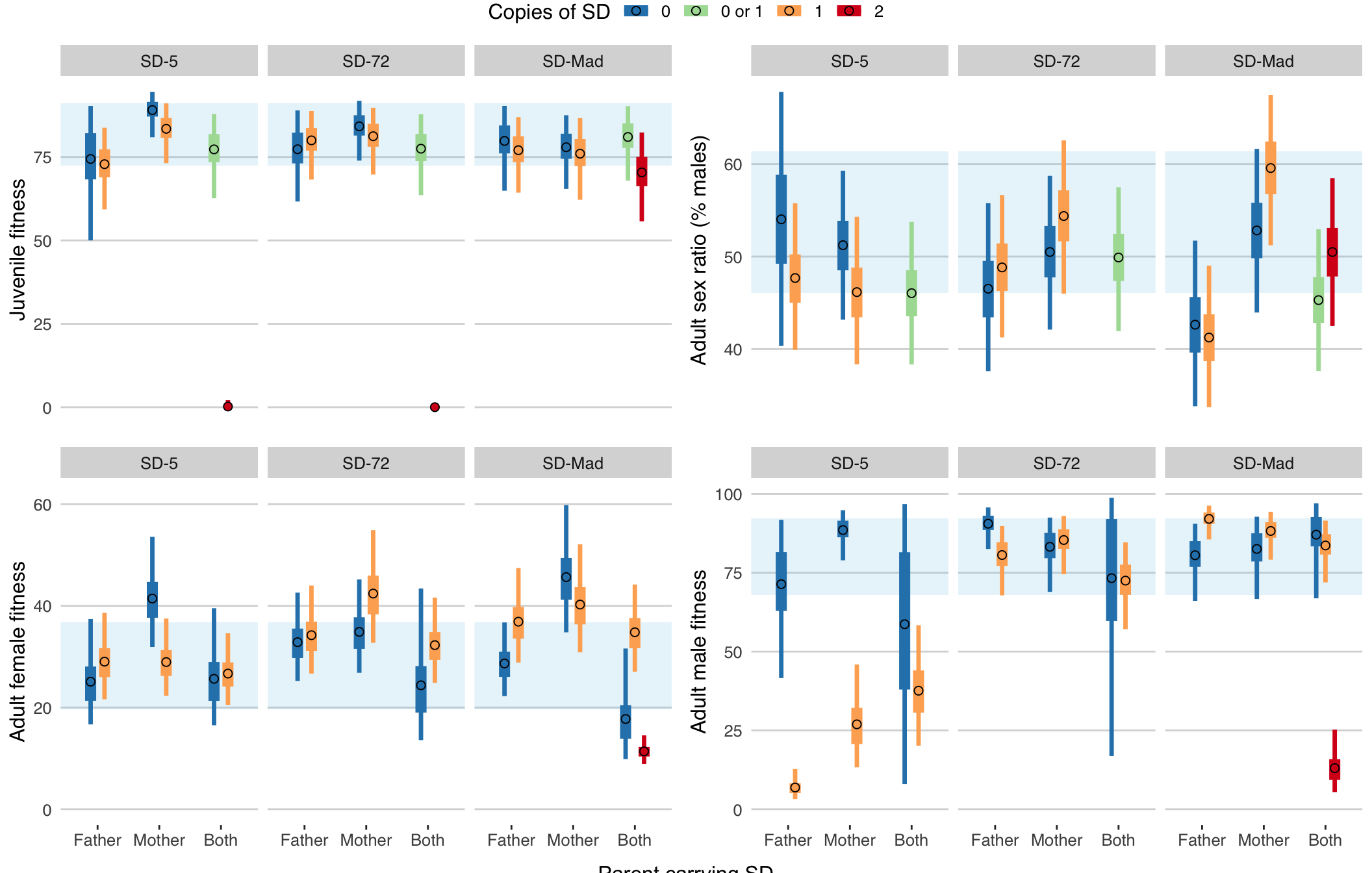
ggsave(fig1, file = "figures/fig1.pdf", height = 7, width = 11)Figure 1: Posterior estimates of the group means for the four different response variables in Experiment 1, for each type of cross (x-axis), SD variant (panels), and genotype (colours). The horizontal blue bar shows the 95% CIs for the sex ratio in the control cross between two SD-free parents, and the error bars show the 95% quantiles of the posterior. Tables S6-S9 give the accompanying statistcal results. Points labelled as carrying “0 or 1” SD allele refer to cases where the genotype of the offspring could not be ascertained due to the brown eye marker not being expressed in larvae; most of these individuals probably carried 1 SD allele because of segregation distortion.
Making Table 1
Table 1: List of the all the notable differences between groups in Experiment 1 (posterior probability <0.05; see Tables S6-S9 for the remaining results). For each contast, we give the parent carrying SD (neither, mother, father, or both) and the number of SD} alleles carried by the offspring. The difference in means is expressed in the original units, i.e. % larvae surviving, % male larvae, number of larvae produced, or % offspring sired, and the parentheses give 95% credible intervals. The difference is positive when the first-listed mean is larger than the second-listed mean, and negative otherwise. The posterior probability (p) has a similar interpretation to a one-tailed p-value.
table1 <- bind_rows(tests1 %>% mutate(Trait = "Larval survival"),
                    tests2 %>% mutate(Trait = "Sex ratio"),
                    tests3 %>% mutate(Trait = "Female fitness"),
                    tests4 %>% mutate(Trait = "Male fitness")) %>%
  filter(Notable == "*") %>% clean_table()

write_csv(table1 %>% rename(p = `Posterior probability`), path = "figures/Table1.csv")
table1 %>% pander(split.cell = 50, split.table = Inf) | Trait | SD | Comparison | Difference | Error | Posterior probability |
|---|---|---|---|---|---|
| Larval survival | SD-5 | Both parents, 0 or 1 - Both parents, 2 | 77.1 ( 62.2 to 87.8) | 6.5 | 0 |
| Larval survival | SD-72 | Both parents, 0 or 1 - Both parents, 2 | 77.5 ( 63.6 to 87.8) | 6.1 | 0 |
| Sex ratio | SD-Mad | Neither, 0 - Father, 0 | 11.1 ( -0.8 to 23.0) | 6.0 | 0.03387 |
| Sex ratio | SD-Mad | Mother, 1 - Father, 1 | 18.3 ( 7.1 to 29.7) | 5.7 | 0.001375 |
| Female fitness | SD-5 | Neither, 0 - Mother, 0 | -14.4 (-28.6 to -0.4) | 7.0 | 0.02187 |
| Female fitness | SD-Mad | Neither, 0 - Mother, 0 | -18.7 (-34.7 to -3.8) | 7.8 | 0.005875 |
| Female fitness | SD-5 | Mother, 0 - Father, 0 | 16.4 ( 1.0 to 31.0) | 7.6 | 0.01862 |
| Female fitness | SD-Mad | Mother, 0 - Father, 0 | 17.0 ( 3.2 to 32.6) | 7.5 | 0.008625 |
| Female fitness | SD-5 | Mother, 0 - Mother, 1 | 12.5 ( -0.2 to 26.1) | 6.6 | 0.02687 |
| Female fitness | SD-Mad | Both parents, 1 - Both parents, 2 | 23.4 ( 15.0 to 33.1) | 4.6 | 0 |
| Male fitness | SD-5 | Mother, 1 - Father, 1 | 20.0 ( 5.5 to 39.2) | 8.8 | 0.003375 |
| Male fitness | SD-5 | Mother, 0 - Mother, 1 | 61.6 ( 41.0 to 77.7) | 9.4 | 0 |
| Male fitness | SD-5 | Father, 0 - Father, 1 | 64.5 ( 34.6 to 85.6) | 13.5 | 0 |
| Male fitness | SD-Mad | Father, 0 - Father, 1 | -11.5 (-26.7 to 0.6) | 6.9 | 0.03213 |
| Male fitness | SD-Mad | Both parents, 1 - Both parents, 2 | 70.6 ( 54.2 to 82.6) | 7.2 | 0 |
Experiment 2
Run a Bayesian binomial generalised linear mixed model
# Function to simular the missing genotypes of embryos that died, assuming fair meiosis in SD mothers and k = k in SD fathers
simulate_expt2_data <- function(expt2_dataset, k){

  have_SD_mum <- which(expt2_dataset$SD_parent == "mum")
  have_SD_dad <- which(expt2_dataset$SD_parent == "dad")

  expt2_dataset$SD_embryos[have_SD_mum] <- with(expt2_dataset[have_SD_mum, ],
                                                SD_offspring + rbinom(length(SD_embryos), Dead_offspring, 0.5))

  expt2_dataset$SD_embryos[have_SD_dad] <- with(expt2_dataset[have_SD_dad, ],
                                                SD_offspring + rbinom(length(SD_embryos), Dead_offspring, k))

  expt2_dataset <- expt2_dataset %>%
    mutate(SD_embryos = as.numeric(SD_embryos),
           CyO_embryos = starting_number_focal_sex - SD_embryos) %>%
    select(-starting_number_focal_sex, -Dead_offspring)

  expt2_dataset %>%
    select(sex_of_embryos, SD, SD_parent, vial, block, SD_offspring, CyO_offspring) %>%
    tidyr::gather(genotype, num_survivors, SD_offspring, CyO_offspring) %>%
    mutate(genotype = gsub("_offspring", "", genotype)) %>%
    left_join(expt2_dataset %>%
                select(sex_of_embryos, SD, SD_parent, vial, block, SD_embryos, CyO_embryos) %>%
                tidyr::gather(genotype, total_number, SD_embryos, CyO_embryos) %>%
                mutate(genotype = gsub("_embryos", "", genotype))) %>%
    arrange(vial)
}

# Simulate some data and run the Bayesian GLMM
model_simulated_data <- function(expt2_dataset, k){

  # First re-format teh data and simulate the missing embryo genotypes using stated value of k
  dat <- simulate_expt2_data(expt2_dataset, k)

  # Now run the model
  brm(num_survivors  | trials(total_number) ~ genotype * sex_of_embryos * SD * SD_parent + (1 | vial),
      data = dat, family = "binomial",
      chains = 4, cores = nCores, seed = 1,
      prior = prior(normal(0, 5), class = "b"),
      control = list(adapt_delta = 0.9999, max_treedepth = 15))

}

# Do the same model for k = 0.5, 0.6 and 0.7
if(!file.exists("data/model_output/expt2_brms.rds")){
  model_list <- list(
    model_simulated_data(expt2, 0.5),
    model_simulated_data(expt2, 0.6),
    model_simulated_data(expt2, 0.7))

  saveRDS(model_list, "data/model_output/expt2_brms.rds")
} else model_list <- readRDS("data/model_output/expt2_brms.rds")
Check a diagnostic plot of the model
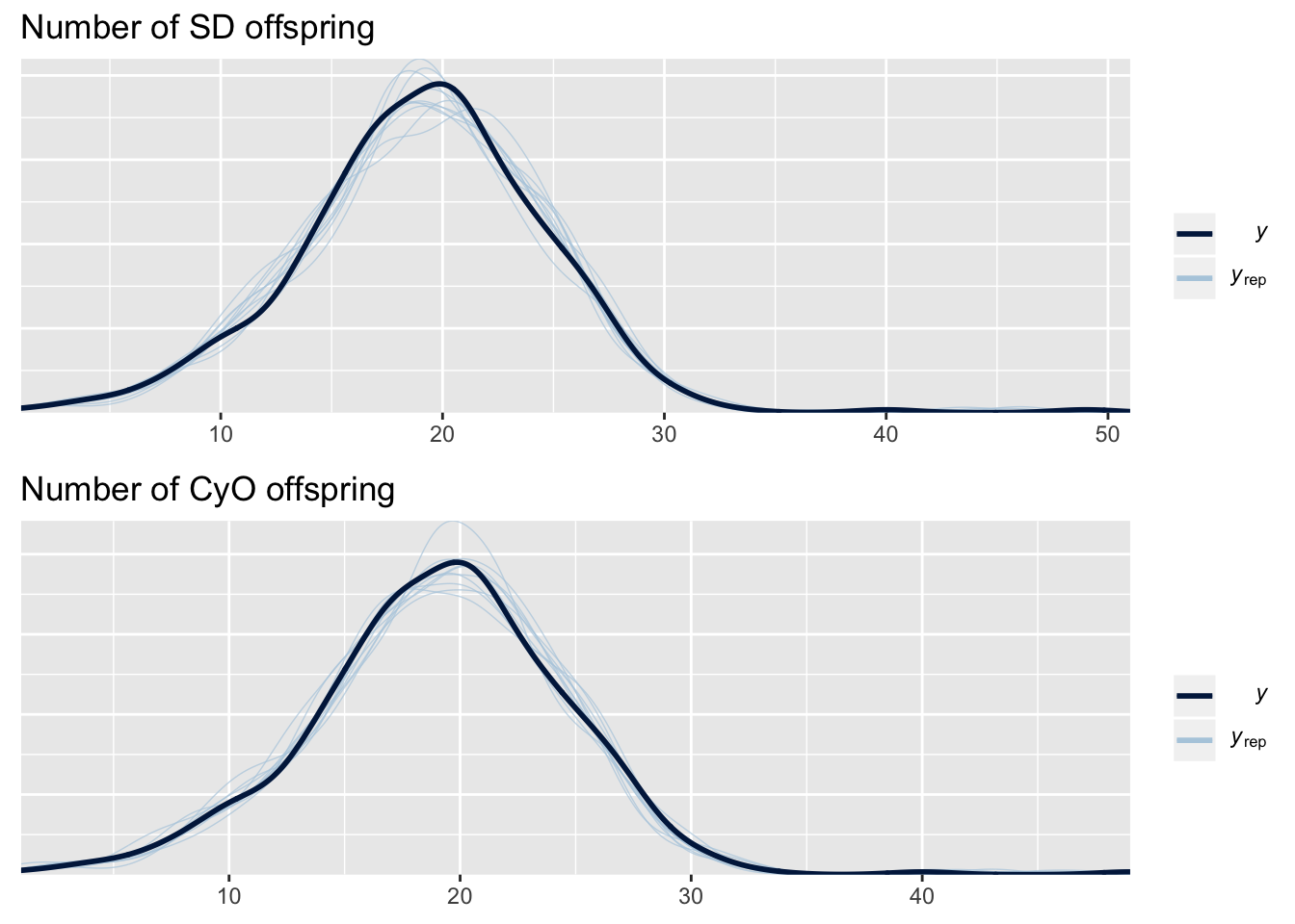
This plot shows the frequency distribution of the original data (black line), along with predicted data that were computed using 10 random samples from the posterior of the model parameters. The posterior predicted values closely match the originals, suggesting that the model is approximating the data reasonably well. There are two plots for this model because we used a multivariate model that jointly modelled two response variables: the survival of SD larvae and of CyO larvae.
grid.arrange(
  pp_check(model_list[[1]], resp = "SDoffspring")  + labs(title = "Number of SD offspring"),
  pp_check(model_list[[1]], resp = "CyOoffspring") + labs(title = "Number of CyO offspring")
)
| Version | Author | Date |
|---|---|---|
| 6b03f9c | lukeholman | 2019-03-12 |
Inspect the model summary
This summary shows the median, error, and 95% CIs for the posterior for all the fixed effects. This table is difficult to interpret and not very informative, but is presented here for completeness.
summarise_brms(model_list[[1]])| Covariate | Estimate | Est.Error | l-95% CI | u-95% CI | Notable |
|---|---|---|---|---|---|
| Intercept | 1.80 | 0.21 | 1.40 | 2.21 | * |
| genotypeSD | -0.10 | 0.20 | -0.49 | 0.28 | |
| sex_of_embryosmale | -0.19 | 0.29 | -0.76 | 0.37 | |
| SDSD-72 | 0.16 | 0.30 | -0.42 | 0.74 | |
| SDSD-Mad | 0.10 | 0.35 | -0.58 | 0.77 | |
| SD_parentmum | -0.19 | 0.28 | -0.74 | 0.37 | |
| genotypeSD:sex_of_embryosmale | -0.17 | 0.27 | -0.70 | 0.36 | |
| genotypeSD:SDSD-72 | 0.07 | 0.29 | -0.49 | 0.65 | |
| genotypeSD:SDSD-Mad | 0.16 | 0.33 | -0.49 | 0.82 | |
| sex_of_embryosmale:SDSD-72 | -0.34 | 0.42 | -1.14 | 0.52 | |
| sex_of_embryosmale:SDSD-Mad | 0.28 | 0.50 | -0.70 | 1.25 | |
| genotypeSD:SD_parentmum | -0.21 | 0.26 | -0.71 | 0.32 | |
| sex_of_embryosmale:SD_parentmum | -0.45 | 0.39 | -1.20 | 0.33 | |
| SDSD-72:SD_parentmum | 0.30 | 0.41 | -0.50 | 1.10 | |
| SDSD-Mad:SD_parentmum | 0.44 | 0.45 | -0.41 | 1.31 | |
| genotypeSD:sex_of_embryosmale:SDSD-72 | 0.34 | 0.40 | -0.45 | 1.13 | |
| genotypeSD:sex_of_embryosmale:SDSD-Mad | -0.09 | 0.47 | -1.00 | 0.83 | |
| genotypeSD:sex_of_embryosmale:SD_parentmum | 0.32 | 0.35 | -0.36 | 1.01 | |
| genotypeSD:SDSD-72:SD_parentmum | 0.49 | 0.38 | -0.26 | 1.23 | |
| genotypeSD:SDSD-Mad:SD_parentmum | -0.34 | 0.42 | -1.18 | 0.48 | |
| sex_of_embryosmale:SDSD-72:SD_parentmum | 0.16 | 0.54 | -0.93 | 1.24 | |
| sex_of_embryosmale:SDSD-Mad:SD_parentmum | -0.40 | 0.61 | -1.58 | 0.78 | |
| genotypeSD:sex_of_embryosmale:SDSD-72:SD_parentmum | -0.54 | 0.51 | -1.52 | 0.46 | |
| genotypeSD:sex_of_embryosmale:SDSD-Mad:SD_parentmum | 0.62 | 0.57 | -0.47 | 1.73 |
Plot the posterior predictions of the group means
new_data <- simulate_expt2_data(expt2, 0.5) %>%
  select(sex_of_embryos, SD, SD_parent, genotype) %>%
  distinct() %>% mutate(total_number = 100) %>%
  arrange(desc(SD_parent), SD, desc(sex_of_embryos))

plot_expt2 <- function(model){

  pd <- position_dodge(0.4)

  predictions <- fitted(model,
                        summary = TRUE,
                        newdata = new_data, re_formula = NA)

  inner_bar <- fitted(model,
                      summary = TRUE,
                      newdata = new_data, re_formula = NA,
                      probs = c(0.25, 0.75))

  process_preds <- function(preds){
    data.frame(new_data, preds) %>%
      rename(Offspring_type = genotype) %>%
      mutate(sex_of_embryos  = str_replace_all(sex_of_embryos, "female", "daughters"),
             sex_of_embryos  = str_replace_all(sex_of_embryos, "male", "sons"),
             Offspring_type = paste(Offspring_type, sex_of_embryos),
             SD_parent = str_replace_all(SD_parent, "dad", "SD/CyO father"),
             SD_parent = str_replace_all(SD_parent, "mum", "SD/CyO mother"))
  }

  left_join(process_preds(predictions),
            process_preds(inner_bar)) %>%
    ggplot(aes(Offspring_type, Estimate, colour = SD_parent, fill = SD_parent)) +
    geom_errorbar(aes(ymin = Q2.5, ymax = Q97.5), width = 0, position = pd, size = 1.3) +
    geom_errorbar(aes(ymin = Q25, ymax = Q75), width = 0, position = pd, size = 3) +
    geom_point(position = pd, size = 2, colour = "black",  pch = 21) +
    facet_grid(~SD) +
    scale_colour_brewer(name = "Cross", palette = "Pastel1", direction = -1, aesthetics = c("colour", "fill")) +
    theme_hc() +
    theme(axis.text.x = element_text(angle = 45, vjust = 1, hjust = 1),
          legend.position = "top", axis.ticks.y = element_blank()) +
    ylab("Juvenile fitness") + xlab("Genotype and sex of offspring")
}

fig2 <- plot_expt2(model_list[[1]])
ggsave(fig2, file = "figures/fig2.pdf", height = 3.9, width = 7)
fig2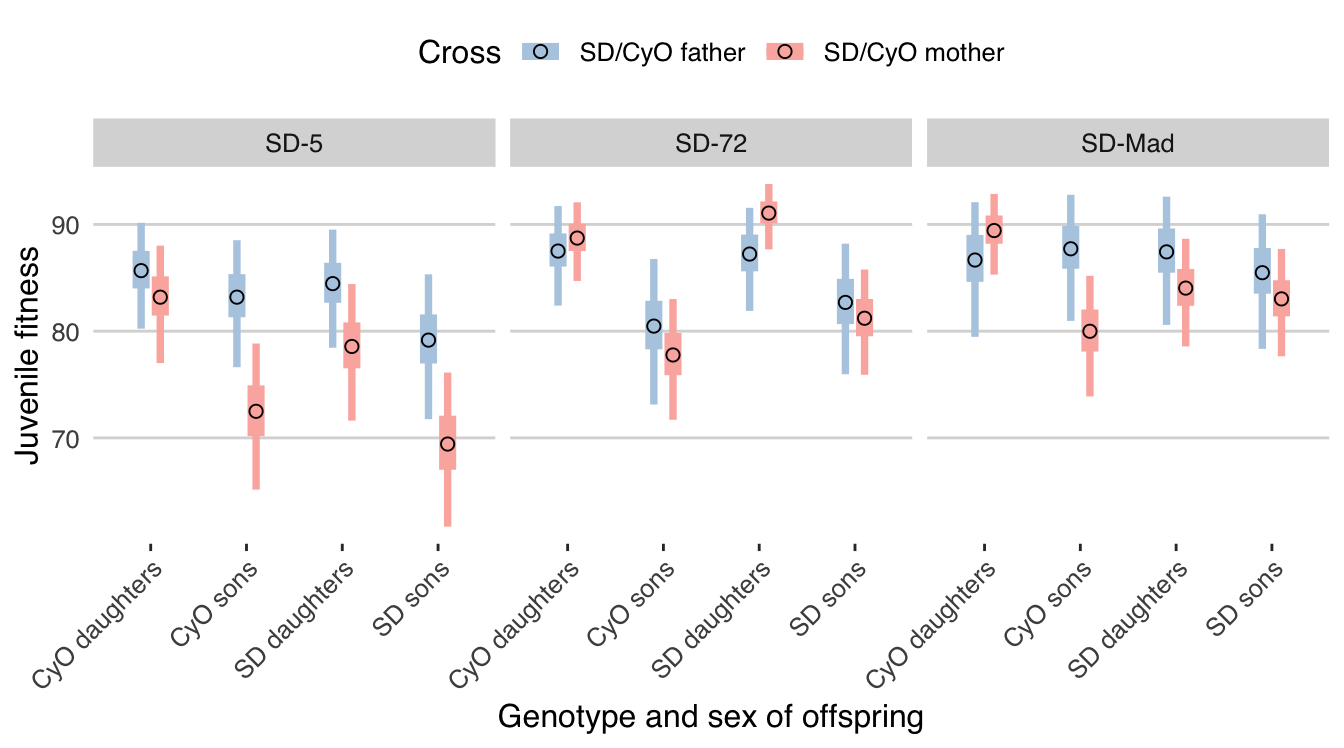
| Version | Author | Date |
|---|---|---|
| 6b03f9c | lukeholman | 2019-03-12 |
Figure 2: Posterior estimates of % L1 larva-to-adult survival in Experiment 2 for each combination of offspring sex and genotype (x-axis), SD variant (panels), and cross (colours). Error bars show the 95% quantiles of the posterior. See Tables 2 and S10 for associated hypothesis tests. This plot was generated assuming fair meiosis (\(k\) = 0.5) in SD/CyO males; see Figure S1 for equivalent plots made using different assumed values of \(k\).
Check the effect of our assumption that meiosis is fair in SD/CyO males
make_expt2_multiplot <- function(...) {
    plots <- list(...)
    g <- ggplotGrob(plots[[1]] + theme(legend.position="bottom"))$grobs
    legend <- g[[which(sapply(g, function(x) x$name) == "guide-box")]]
    lheight <- sum(legend$height)
    plots <- lapply(plots, function(x) ggplotGrob(x + theme(legend.position = "none")))

    p <- gtable_rbind(plots[[1]], plots[[2]], plots[[3]])

    grid.arrange(p, legend,
                 nrow = 2,
                 heights = unit.c(unit(1, "npc") - lheight, lheight))
  }

make_expt2_multiplot(
  plot_expt2(model_list[[1]]) + theme(axis.text.x = element_blank(), axis.ticks.x = element_blank()) + xlab(NULL) + ylab(NULL),
  plot_expt2(model_list[[2]]) + theme(axis.text.x = element_blank(), axis.ticks.x = element_blank()) + xlab(NULL),
  plot_expt2(model_list[[3]]) + ylab(NULL))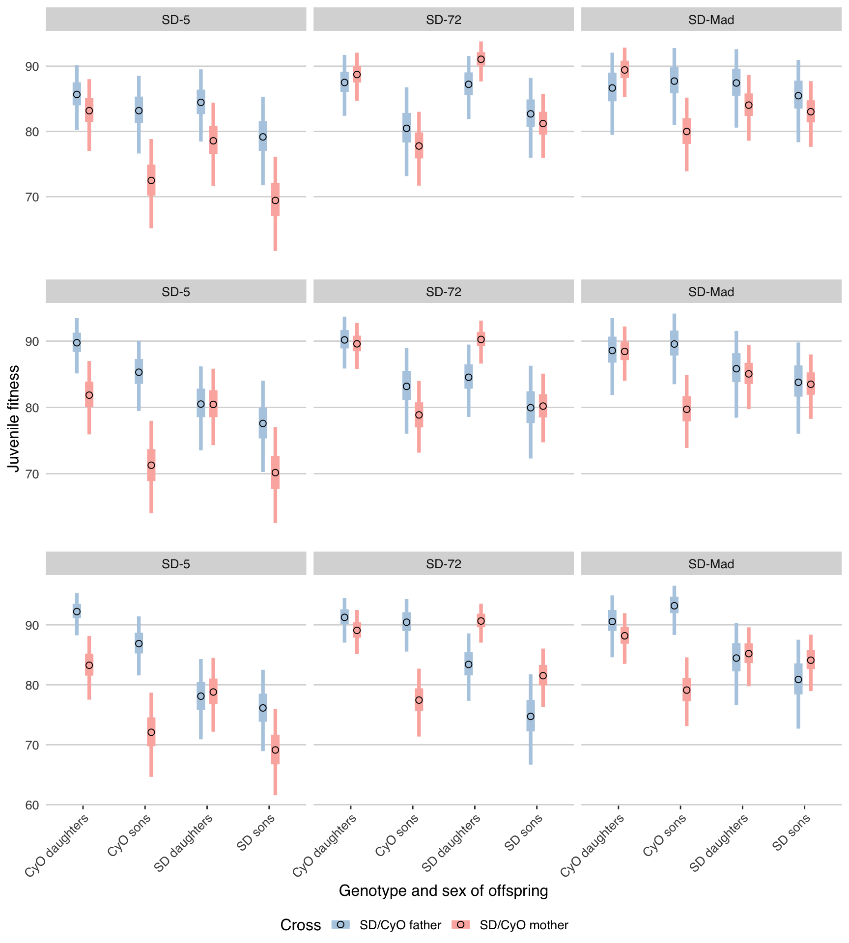
| Version | Author | Date |
|---|---|---|
| 6b03f9c | lukeholman | 2019-03-12 |
Figure S1: Equivalent plots to Figure 2, under the assumption that meiosis is fair (\(k\) = 0.5, top row, same as Figure 2), slightly biased (\(k\) = 0.6, middle row), and more strongly biased (\(k\) = 0.7, bottom row). Note that the significant results for Figure 2 mostly stay the same or increase in magnitude, suggesting that they are genuine and are not sensitive to our assumptions about the data.
Hypothesis testing
hypothesis_tests_expt2 <- function(model){

  compare <- function(mean1, mean2, SD, Mean_1, Mean_2){
  difference <- mean1 - mean2
  prob_less <- hypothesis(data.frame(x = difference), "x < 0")$hypothesis
  prob_more <- hypothesis(data.frame(x = difference), "x > 0")$hypothesis
  output <- data.frame(
    SD, Mean_1, Mean_2,
    hypothesis(data.frame(x = difference), "x = 0")$hypothesis %>%
    mutate(Posterior_probability = min(c(prob_less$Post.Prob, prob_more$Post.Prob)),
           Evidence_ratio = max(c(prob_less$Evid.Ratio, prob_more$Evid.Ratio)))
  )
}
  preds <- fitted(model,
                  summary = FALSE,
                  newdata = new_data, re_formula = NA)


  SD5_sons_mum_SD <- preds[,1]
  SD5_sons_mum_CyO <- preds[,2]
  SD5_daughters_mum_SD <- preds[,3]
  SD5_daughters_mum_CyO <- preds[,4]
  SD72_sons_mum_SD <- preds[,5]
  SD72_sons_mum_CyO <- preds[,6]
  SD72_daughters_mum_SD <- preds[,7]
  SD72_daughters_mum_CyO <- preds[,8]
  SDMad_sons_mum_SD <- preds[,9]
  SDMad_sons_mum_CyO <- preds[,10]
  SDMad_daughters_mum_SD <- preds[,11]
  SDMad_daughters_mum_CyO <- preds[,12]
  SD5_sons_dad_SD <- preds[,13]
  SD5_sons_dad_CyO <- preds[,14]
  SD5_daughters_dad_SD <- preds[,15]
  SD5_daughters_dad_CyO <- preds[,16]
  SD72_sons_dad_SD <- preds[,17]
  SD72_sons_dad_CyO <- preds[,18]
  SD72_daughters_dad_SD <- preds[,19]
  SD72_daughters_dad_CyO <- preds[,20]
  SDMad_sons_dad_SD <- preds[,21]
  SDMad_sons_dad_CyO <- preds[,22]
  SDMad_daughters_dad_SD <- preds[,23]
  SDMad_daughters_dad_CyO <- preds[,24]

  rbind(
    # sex effect on SD individuals when mother has SD
    compare(SD5_sons_mum_SD, SD5_daughters_mum_SD, "SD-5", "Sons, SD, mother", "Daughters, SD, mother"),
    compare(SD72_sons_mum_SD, SD72_daughters_mum_SD, "SD-72", "Sons, SD, mother", "Daughters, SD, mother"),
    compare(SDMad_sons_mum_SD, SDMad_daughters_mum_SD, "SD-Mad", "Sons, SD, mother", "Daughters, SD, mother"),
    # sex effect on CyO individuals when mother has SD
    compare(SD5_sons_mum_CyO, SD5_daughters_mum_CyO, "SD-5", "Sons, CyO, mother", "Daughters, CyO, mother"),
    compare(SD72_sons_mum_CyO, SD72_daughters_mum_CyO, "SD-72", "Sons, CyO, mother", "Daughters, CyO, mother"),
    compare(SDMad_sons_mum_CyO, SDMad_daughters_mum_CyO, "SD-Mad", "Sons, CyO, mother", "Daughters, CyO, mother"),
    # sex effect on SD individuals when father has SD
    compare(SD5_sons_dad_SD, SD5_daughters_dad_SD, "SD-5", "Sons, SD, father", "Daughters, SD, father"),
    compare(SD72_sons_dad_SD, SD72_daughters_dad_SD, "SD-72", "Sons, SD, father", "Daughters, SD, father"),
    compare(SDMad_sons_dad_SD, SDMad_daughters_dad_SD, "SD-Mad", "Sons, SD, father", "Daughters, SD, father"),
    # sex effect on CyO individuals when father has SD
    compare(SD5_sons_dad_CyO, SD5_daughters_dad_CyO, "SD-5", "Sons, CyO, father", "Daughters, CyO, father"),
    compare(SD72_sons_dad_CyO, SD72_daughters_dad_CyO, "SD-72", "Sons, CyO, father", "Daughters, CyO, father"),
    compare(SDMad_sons_dad_CyO, SDMad_daughters_dad_CyO, "SD-Mad", "Sons, CyO, father", "Daughters, CyO, father"),
    # effect of inheriting SD not CyO from mother on sons
    compare(SD5_sons_mum_CyO, SD5_sons_mum_SD, "SD-5", "Sons, CyO, mother", "Sons, SD, mother"),
    compare(SD72_sons_mum_CyO, SD72_sons_mum_SD, "SD-72", "Sons, CyO, mother", "Sons, SD, mother"),
    compare(SDMad_sons_mum_CyO, SDMad_sons_mum_SD, "SD-Mad", "Sons, CyO, mother", "Sons, SD, mother"),
    # effect of inheriting SD not CyO from father on sons
    compare(SD5_sons_dad_CyO, SD5_sons_dad_SD, "SD-5", "Sons, CyO, father", "Sons, SD, father"),
    compare(SD72_sons_dad_CyO, SD72_sons_dad_SD, "SD-72", "Sons, CyO, father", "Sons, SD, father"),
    compare(SDMad_sons_dad_CyO, SDMad_sons_dad_SD, "SD-Mad", "Sons, CyO, father", "Sons, SD, father"),
    # effect of inheriting SD not CyO from mother on daughters
    compare(SD5_daughters_mum_CyO, SD5_daughters_mum_SD, "SD-5", "Daughters, CyO, mother", "Daughters, SD, mother"),
    compare(SD72_daughters_mum_CyO, SD72_daughters_mum_SD, "SD-72", "Daughters, CyO, mother", "Daughters, SD, mother"),
    compare(SDMad_daughters_mum_CyO, SDMad_daughters_mum_SD, "SD-Mad", "Daughters, CyO, mother", "Daughters, SD, mother"),
    # effect of inheriting SD not CyO from father on daughters
    compare(SD5_daughters_dad_CyO, SD5_daughters_dad_SD, "SD-5", "Daughters, CyO, father", "Daughters, SD, father"),
    compare(SD72_daughters_dad_CyO, SD72_daughters_dad_SD, "SD-72", "Daughters, CyO, father", "Daughters, SD, father"),
    compare(SDMad_daughters_dad_CyO, SDMad_daughters_dad_SD, "SD-Mad", "Daughters, CyO, father", "Daughters, SD, father"),
    # effect of cross direction for SD sons
    compare(SD5_sons_mum_SD, SD5_sons_dad_SD, "SD-5", "Sons, SD, mother", "Sons, SD, father"),
    compare(SD72_sons_mum_SD, SD72_sons_dad_SD, "SD-72", "Sons, SD, mother", "Sons, SD, father"),
    compare(SDMad_sons_mum_SD, SDMad_sons_dad_SD, "SD-Mad", "Sons, SD, mother", "Sons, SD, father"),
    # effect of cross direction for SD daughters
    compare(SD5_daughters_mum_SD, SD5_daughters_dad_SD, "SD-5", "Daughters, SD, mother", "Daughters, SD, father"),
    compare(SD72_daughters_mum_SD, SD72_daughters_dad_SD, "SD-72", "Daughters, SD, mother", "Daughters, SD, father"),
    compare(SDMad_daughters_mum_SD, SDMad_daughters_dad_SD, "SD-Mad", "Daughters, SD, mother", "Daughters, SD, father"),
    # effect of cross direction for CyO sons
    compare(SD5_sons_mum_CyO, SD5_sons_dad_CyO, "SD-5", "Sons, CyO, mother", "Sons, CyO, father"),
    compare(SD72_sons_mum_CyO, SD72_sons_dad_CyO, "SD-72", "Sons, CyO, mother", "Sons, CyO, father"),
    compare(SDMad_sons_mum_CyO, SDMad_sons_dad_CyO, "SD-Mad", "Sons, CyO, mother", "Sons, CyO, father"),
    # effect of cross direction for CyO daughters
    compare(SD5_daughters_mum_CyO, SD5_daughters_dad_CyO, "SD-5", "Daughters, CyO, mother", "Daughters, CyO, father"),
    compare(SD72_daughters_mum_CyO, SD72_daughters_dad_CyO, "SD-72", "Daughters, CyO, mother", "Daughters, CyO, father"),
    compare(SDMad_daughters_mum_CyO, SDMad_daughters_dad_CyO, "SD-Mad", "Daughters, CyO, mother", "Daughters, CyO, father")
  ) %>%
    select(-Hypothesis, -Evid.Ratio, -Post.Prob, -Star) %>%
    mutate(Notable = ifelse(Posterior_probability < 0.05, "*", ""),
           Test = c(rep("Sex difference in survival", 12),
                    rep("Effect of offspring genotype", 12),
                    rep("Effect of parental genotype", 12))) %>% as_tibble()
}

tests_expt2 <- hypothesis_tests_expt2(model_list[[1]]) %>%
  mutate(Estimate = format(round(Estimate, 1), nsmall = 1),
         Est.Error = format(round(Est.Error, 1), nsmall = 1),
         CI.Lower = format(round(CI.Lower, 1), nsmall = 1),
         CI.Upper = format(round(CI.Upper, 1), nsmall = 1),
         Difference = paste(Estimate, " (", CI.Lower, " to ", CI.Upper, ")", sep = ""),
         Comparison = paste(Mean_1, "-", Mean_2),
         Error = Est.Error) %>%
  select(SD, Comparison, Difference, Error, Posterior_probability, Notable) %>%
  arrange(SD, Comparison)
Table 2: List of the all the notable differences between groups in Experiment 2 (posterior probability $<$0.05; see Table S10 for the remaining results). For each group, we list the sex of the focal larvae, their genotype (SD or CyO), and the parent that carried SD (mother or father). The difference in means is expressed in % larvae surviving; other details are as in Table 1.
table2 <- tests_expt2 %>%
  filter(Notable == "*") %>% select(-Notable)
names(table2) <- str_replace_all(names(table2), "_", " ")

write_csv(table2 %>% rename(p = `Posterior probability`), path = "figures/Table2.csv")
table2 %>% pander(split.cell = 50, split.table = Inf)| SD | Comparison | Difference | Error | Posterior probability |
|---|---|---|---|---|
| SD-5 | Daughters, CyO, mother - Daughters, SD, mother | 4.6 ( -0.6 to 10.0) | 2.7 | 0.041 |
| SD-5 | Sons, CyO, mother - Daughters, CyO, mother | -10.7 (-19.4 to -2.0) | 4.5 | 0.00825 |
| SD-5 | Sons, CyO, mother - Sons, CyO, father | -10.7 (-19.8 to -1.5) | 4.6 | 0.0105 |
| SD-5 | Sons, SD, mother - Daughters, SD, mother | -9.1 (-18.7 to 0.4) | 4.8 | 0.028 |
| SD-5 | Sons, SD, mother - Sons, SD, father | -9.7 (-19.4 to -0.1) | 5.0 | 0.02475 |
| SD-72 | Sons, CyO, father - Daughters, CyO, father | -7.0 (-15.5 to 1.0) | 4.2 | 0.04475 |
| SD-72 | Sons, CyO, mother - Daughters, CyO, mother | -11.0 (-17.9 to -4.3) | 3.5 | 0.00075 |
| SD-72 | Sons, SD, mother - Daughters, SD, mother | -9.9 (-15.8 to -4.2) | 3.0 | 5e-04 |
| SD-Mad | Daughters, CyO, mother - Daughters, SD, mother | 5.4 ( 1.2 to 9.9) | 2.2 | 0.00675 |
| SD-Mad | Sons, CyO, mother - Daughters, CyO, mother | -9.4 (-16.3 to -2.7) | 3.5 | 0.00225 |
| SD-Mad | Sons, CyO, mother - Sons, CyO, father | -7.7 (-15.6 to 0.6) | 4.1 | 0.0345 |
Table S10: Complete version of Table 2, showing all the contrasts that were tested in Experiment 2.
tests_expt2 %>% pander(split.cell = 50, split.table = Inf) | SD | Comparison | Difference | Error | Posterior_probability | Notable |
|---|---|---|---|---|---|
| SD-5 | Daughters, CyO, father - Daughters, SD, father | 1.2 ( -3.5 to 6.3) | 2.5 | 0.3105 | |
| SD-5 | Daughters, CyO, mother - Daughters, CyO, father | -2.5 ( -9.8 to 4.8) | 3.7 | 0.2448 | |
| SD-5 | Daughters, CyO, mother - Daughters, SD, mother | 4.6 ( -0.6 to 10.0) | 2.7 | 0.041 | * |
| SD-5 | Daughters, SD, mother - Daughters, SD, father | -5.9 (-14.6 to 2.5) | 4.2 | 0.07775 | |
| SD-5 | Sons, CyO, father - Daughters, CyO, father | -2.5 (-10.4 to 4.9) | 3.9 | 0.2597 | |
| SD-5 | Sons, CyO, father - Sons, SD, father | 4.0 ( -1.8 to 10.0) | 3.0 | 0.08675 | |
| SD-5 | Sons, CyO, mother - Daughters, CyO, mother | -10.7 (-19.4 to -2.0) | 4.5 | 0.00825 | * |
| SD-5 | Sons, CyO, mother - Sons, CyO, father | -10.7 (-19.8 to -1.5) | 4.6 | 0.0105 | * |
| SD-5 | Sons, CyO, mother - Sons, SD, mother | 3.1 ( -2.8 to 9.0) | 3.0 | 0.1493 | |
| SD-5 | Sons, SD, father - Daughters, SD, father | -5.3 (-14.5 to 3.7) | 4.5 | 0.118 | |
| SD-5 | Sons, SD, mother - Daughters, SD, mother | -9.1 (-18.7 to 0.4) | 4.8 | 0.028 | * |
| SD-5 | Sons, SD, mother - Sons, SD, father | -9.7 (-19.4 to -0.1) | 5.0 | 0.02475 | * |
| SD-72 | Daughters, CyO, father - Daughters, SD, father | 0.3 ( -4.4 to 5.0) | 2.4 | 0.449 | |
| SD-72 | Daughters, CyO, mother - Daughters, CyO, father | 1.2 ( -4.7 to 7.4) | 3.0 | 0.3395 | |
| SD-72 | Daughters, CyO, mother - Daughters, SD, mother | -2.3 ( -5.9 to 1.1) | 1.8 | 0.0875 | |
| SD-72 | Daughters, SD, mother - Daughters, SD, father | 3.8 ( -1.6 to 9.9) | 2.9 | 0.08525 | |
| SD-72 | Sons, CyO, father - Daughters, CyO, father | -7.0 (-15.5 to 1.0) | 4.2 | 0.04475 | * |
| SD-72 | Sons, CyO, father - Sons, SD, father | -2.2 ( -8.8 to 3.8) | 3.2 | 0.2433 | |
| SD-72 | Sons, CyO, mother - Daughters, CyO, mother | -11.0 (-17.9 to -4.3) | 3.5 | 0.00075 | * |
| SD-72 | Sons, CyO, mother - Sons, CyO, father | -2.7 (-11.4 to 6.3) | 4.5 | 0.2742 | |
| SD-72 | Sons, CyO, mother - Sons, SD, mother | -3.4 ( -8.1 to 1.2) | 2.4 | 0.074 | |
| SD-72 | Sons, SD, father - Daughters, SD, father | -4.5 (-12.7 to 3.3) | 4.1 | 0.1335 | |
| SD-72 | Sons, SD, mother - Daughters, SD, mother | -9.9 (-15.8 to -4.2) | 3.0 | 5e-04 | * |
| SD-72 | Sons, SD, mother - Sons, SD, father | -1.5 ( -9.3 to 6.4) | 4.1 | 0.354 | |
| SD-Mad | Daughters, CyO, father - Daughters, SD, father | -0.8 ( -6.9 to 5.2) | 3.1 | 0.4085 | |
| SD-Mad | Daughters, CyO, mother - Daughters, CyO, father | 2.8 ( -4.3 to 10.7) | 3.8 | 0.236 | |
| SD-Mad | Daughters, CyO, mother - Daughters, SD, mother | 5.4 ( 1.2 to 9.9) | 2.2 | 0.00675 | * |
| SD-Mad | Daughters, SD, mother - Daughters, SD, father | -3.4 (-11.0 to 4.9) | 4.0 | 0.1965 | |
| SD-Mad | Sons, CyO, father - Daughters, CyO, father | 1.1 ( -7.8 to 9.8) | 4.5 | 0.4127 | |
| SD-Mad | Sons, CyO, father - Sons, SD, father | 2.2 ( -4.1 to 8.7) | 3.2 | 0.2318 | |
| SD-Mad | Sons, CyO, mother - Daughters, CyO, mother | -9.4 (-16.3 to -2.7) | 3.5 | 0.00225 | * |
| SD-Mad | Sons, CyO, mother - Sons, CyO, father | -7.7 (-15.6 to 0.6) | 4.1 | 0.0345 | * |
| SD-Mad | Sons, CyO, mother - Sons, SD, mother | -3.0 ( -8.0 to 1.9) | 2.5 | 0.1115 | |
| SD-Mad | Sons, SD, father - Daughters, SD, father | -1.9 (-10.9 to 6.7) | 4.6 | 0.3347 | |
| SD-Mad | Sons, SD, mother - Daughters, SD, mother | -1.0 ( -8.0 to 6.1) | 3.6 | 0.3847 | |
| SD-Mad | Sons, SD, mother - Sons, SD, father | -2.5 (-10.3 to 6.3) | 4.1 | 0.2578 |
sessionInfo()R version 3.5.1 (2018-07-02)
Platform: x86_64-apple-darwin15.6.0 (64-bit)
Running under: macOS High Sierra 10.13.6
Matrix products: default
BLAS: /Library/Frameworks/R.framework/Versions/3.5/Resources/lib/libRblas.0.dylib
LAPACK: /Library/Frameworks/R.framework/Versions/3.5/Resources/lib/libRlapack.dylib
locale:
[1] en_AU.UTF-8/en_AU.UTF-8/en_AU.UTF-8/C/en_AU.UTF-8/en_AU.UTF-8
attached base packages:
[1] grid stats graphics grDevices utils datasets methods
[8] base
other attached packages:
[1] stringr_1.3.1 tibble_2.0.99.9000 readr_1.1.1
[4] ggthemes_4.0.1 gridExtra_2.3 lazerhawk_0.2.4
[7] pander_0.6.2 Cairo_1.5-9 reshape2_1.4.3
[10] brms_2.6.0 ggplot2_3.1.0 Rcpp_1.0.0
[13] dplyr_0.8.0.1 knitr_1.20
loaded via a namespace (and not attached):
[1] nlme_3.1-137 matrixStats_0.54.0 fs_1.2.6
[4] xts_0.11-0 devtools_1.13.6 RColorBrewer_1.1-2
[7] threejs_0.3.1 rprojroot_1.3-2 rstan_2.18.2
[10] tools_3.5.1 backports_1.1.2 R6_2.4.0
[13] DT_0.4 lazyeval_0.2.1 colorspace_1.3-2
[16] withr_2.1.2 tidyselect_0.2.5 prettyunits_1.0.2
[19] processx_3.2.1 Brobdingnag_1.2-5 compiler_3.5.1
[22] git2r_0.23.0 cli_1.0.1 shinyjs_1.0
[25] labeling_0.3 colourpicker_1.0 scales_1.0.0
[28] dygraphs_1.1.1.6 mvtnorm_1.0-8 ggridges_0.5.0
[31] callr_2.0.4 digest_0.6.18 StanHeaders_2.18.0
[34] rmarkdown_1.10 base64enc_0.1-3 pkgconfig_2.0.2
[37] htmltools_0.3.6 htmlwidgets_1.2 rlang_0.3.1
[40] shiny_1.2.0 zoo_1.8-3 crosstalk_1.0.0
[43] gtools_3.8.1 inline_0.3.15 magrittr_1.5
[46] loo_2.0.0 bayesplot_1.5.0 Matrix_1.2-14
[49] munsell_0.5.0 abind_1.4-5 stringi_1.3.1
[52] whisker_0.3-2 yaml_2.2.0 pkgbuild_1.0.2
[55] plyr_1.8.4 parallel_3.5.1 promises_1.0.1
[58] crayon_1.3.4 miniUI_0.1.1.1 lattice_0.20-35
[61] hms_0.4.2 ps_1.3.0 pillar_1.3.1.9000
[64] igraph_1.2.1 markdown_0.8 shinystan_2.5.0
[67] stats4_3.5.1 rstantools_1.5.0 glue_1.3.0.9000
[70] evaluate_0.11 httpuv_1.4.5 gtable_0.2.0
[73] purrr_0.3.1 tidyr_0.8.2 assertthat_0.2.0
[76] mime_0.6 xtable_1.8-3 colortools_0.1.5
[79] coda_0.19-2 later_0.7.5 rsconnect_0.8.8
[82] shinythemes_1.1.1 memoise_1.1.0 workflowr_1.2.0
[85] bridgesampling_0.4-0