Correcting the GWAS results using multivariate adaptive shrinkage
Last updated: 2021-09-26
Checks: 6 1
Knit directory: fitnessGWAS/
This reproducible R Markdown analysis was created with workflowr (version 1.6.2). The Checks tab describes the reproducibility checks that were applied when the results were created. The Past versions tab lists the development history.
Great! Since the R Markdown file has been committed to the Git repository, you know the exact version of the code that produced these results.
Great job! The global environment was empty. Objects defined in the global environment can affect the analysis in your R Markdown file in unknown ways. For reproduciblity it’s best to always run the code in an empty environment.
The command set.seed(20180914) was run prior to running the code in the R Markdown file. Setting a seed ensures that any results that rely on randomness, e.g. subsampling or permutations, are reproducible.
Great job! Recording the operating system, R version, and package versions is critical for reproducibility.
Nice! There were no cached chunks for this analysis, so you can be confident that you successfully produced the results during this run.
Using absolute paths to the files within your workflowr project makes it difficult for you and others to run your code on a different machine. Change the absolute path(s) below to the suggested relative path(s) to make your code more reproducible.
| absolute | relative |
|---|---|
| /Users/lholman/Rprojects/fitnessGWAS | . |
Great! You are using Git for version control. Tracking code development and connecting the code version to the results is critical for reproducibility.
The results in this page were generated with repository version af15dd6. See the Past versions tab to see a history of the changes made to the R Markdown and HTML files.
Note that you need to be careful to ensure that all relevant files for the analysis have been committed to Git prior to generating the results (you can use wflow_publish or wflow_git_commit). workflowr only checks the R Markdown file, but you know if there are other scripts or data files that it depends on. Below is the status of the Git repository when the results were generated:
Ignored files:
    Ignored:    .DS_Store
    Ignored:    .Rapp.history
    Ignored:    .Rhistory
    Ignored:    .Rproj.user/
    Ignored:    .httr-oauth
    Ignored:    .pversion
    Ignored:    analysis/.DS_Store
    Ignored:    analysis/correlations_SNP_effects_cache/
    Ignored:    code/.DS_Store
    Ignored:    code/Drosophila_GWAS.Rmd
    Ignored:    data/.DS_Store
    Ignored:    data/derived/
    Ignored:    data/input/.DS_Store
    Ignored:    data/input/.pversion
    Ignored:    data/input/dgrp.fb557.annot.txt
    Ignored:    data/input/dgrp2.bed
    Ignored:    data/input/dgrp2.bim
    Ignored:    data/input/dgrp2.fam
    Ignored:    data/input/huang_transcriptome/
    Ignored:    figures/.DS_Store
    Ignored:    figures/fig1_inkscape.svg
    Ignored:    figures/figure1a.pdf
    Ignored:    figures/figure1b.pdf

Untracked files:
    Untracked:  big_model.rds
    Untracked:  code/gcta64
    Untracked:  code/plink
    Untracked:  code/quant_gen_1.R
    Untracked:  data/input/genomic_relatedness_matrix.rds
    Untracked:  figures/SNP_effect_ED.pdf
    Untracked:  figures/boyle_plot.pdf
    Untracked:  figures/fig1.pdf
    Untracked:  manuscript/GWAS_manuscript.log
    Untracked:  old_analyses/

Unstaged changes:
    Modified:   .gitignore
    Deleted:    Rplots.pdf
    Deleted:    analysis/GO_KEGG_enrichment.Rmd
    Deleted:    analysis/plotting_results.Rmd
    Deleted:    code/GO_and_KEGG_gsea.R
    Deleted:    code/make_sites_files_for_ARGweaver.R
    Deleted:    code/plotting_results.Rmd
    Deleted:    code/run_argweaver.R
    Modified:   code/run_mashr.R
    Deleted:    data/input/clough_2014_dsx_targets.csv
    Modified:   figures/GWAS_stats_figure.pdf
    Modified:   figures/TWAS_stats_figure.pdf
    Modified:   figures/antagonism_ratios.pdf
    Modified:   figures/composite_mixture_figure.pdf
    Modified:   figures/eff_size_histos.pdf
    Deleted:    figures/figure1.eps
    Deleted:    figures/figure2.eps
    Modified:   manuscript/GWAS_manuscript.Rmd
    Modified:   manuscript/GWAS_manuscript.pdf
    Modified:   manuscript/GWAS_manuscript.tex
Note that any generated files, e.g. HTML, png, CSS, etc., are not included in this status report because it is ok for generated content to have uncommitted changes.
These are the previous versions of the repository in which changes were made to the R Markdown (analysis/gwas_adaptive_shrinkage.Rmd) and HTML (docs/gwas_adaptive_shrinkage.html) files. If you’ve configured a remote Git repository (see ?wflow_git_remote), click on the hyperlinks in the table below to view the files as they were in that past version.
| File | Version | Author | Date | Message |
|---|---|---|---|---|
| Rmd | af15dd6 | lukeholman | 2021-09-26 | Commit Sept 2021 |
| Rmd | 3855d33 | lukeholman | 2021-03-04 | big fist commit 2021 |
| html | 3855d33 | lukeholman | 2021-03-04 | big fist commit 2021 |
| Rmd | 8d54ea5 | Luke Holman | 2018-12-23 | Initial commit |
| html | 8d54ea5 | Luke Holman | 2018-12-23 | Initial commit |
library(tidyverse)
library(ashr) # Also requires installation of RMosek, which needs a (free) licence. See the ashr Github page for help
library(mashr) # NB: This has multiple dependencies and was tricky to install. Read the Github page, and good luck!
library(glue)
library(kableExtra)
library(gridExtra)


# Get the list of SNPs (or chunks of 100% SNP clumps) that are in approx. LD with one another
get_mashr_data <- function(){

  SNPs_in_LD <- read.table("data/derived/SNPs_in_LD", header = FALSE)

  data_for_mashr <- read_csv("data/derived/all_univariate_GEMMA_results.csv") %>%
    filter(str_detect(SNPs, ",") | SNPs %in% SNPs_in_LD$V1) %>%
    select(SNPs, starts_with("beta"), starts_with("SE"))

  single_snps <- data_for_mashr %>% filter(!str_detect(SNPs, ","))
  multiple_snps <- data_for_mashr %>% filter(str_detect(SNPs, ","))
  multiple_snps <- multiple_snps[enframe(strsplit(multiple_snps$SNPs, split = ", ")) %>%
                                   unnest(value) %>%
                                   filter(value %in% SNPs_in_LD$V1) %>%
                                   pull(name), ]
  bind_rows(single_snps, multiple_snps) %>% arrange(SNPs)
}
Run multivariate adaptive shrinkage using mashr
Whole-genome analyses
This section analyses variants from all chromosomes for which data were available (2L, 2R, 3L, 3R, 4, and X).
The following code runs the package mashr, which attempts to infer more accurate estimates of the true SNP effect sizes (denoted \(\beta\)) by applying shrinkage based on the multivariate structure of the data. mashr accepts a matrix of four \(\beta\) terms for each locus (for the four fitness measures) as well as the four associated standard errors. mashr then uses Bayesian mixture models to estimate the true (i.e. shrinked) \(\beta\) terms, the local false sign rate, the proportion of SNPs that belong to each mixture component, and other useful things. For more information on mashr, see the package website, and the associated paper by Urbut, Wang, and Stephens (doi:10.1101/096552).
Importantly, there are two ways to run mashr: fitting a mixture model that uses “canonical” covariance matrices which are defined a priori by the user, or using covariance matrices that are selected by an algorithm based on the multivariate structure of the raw data. The following code runs both approaches, since they provide complementary information (see Methods in our paper).
In the ‘canonical’ analysis, we were a priori interested in determining the relative abundances of variants that affect fitness in the following list of possible ways:
- null (no effect on fitness)
- uniform effect (the fitness effect of the allele is identical on all sexes and age classes; termed
equal_effectsinmashr) - same sign, variable magnitude (the fitness effect of the allele has the same sign for all sexes and age classes, though its magnitude is variable; termed
simple_hetinmashr) - sexually antagonistic (one allele is good for one sex and bad for the other, though this effect is the same in young and old individuals)
- age antagonistic (one allele is good for one age class and bad for the other, though this effect is the same in males and females)
- female-specific (there is an effect in females but no effect in males; same sign of effect across age classes)
- male-specific (there is an effect in males but no effect in females; same sign of effect across age classes)
- early-life-specific (the locus affects the fitness of young flies of both sexes, but has no effect on old flies)
- late-life-specific (the locus affects the fitness of old flies of both sexes, but has no effect on young flies)
- female-specific effect, with a variable effect across age classes
- male-specific effect, with an effect magnitude and/or sign that changes with age
- female-specific effect, with an effect magnitude and/or sign that changes with age
- early-life-specific effect, with an effect magnitude and/or sign that differs between sexes
- late-life-specific effect, with an effect magnitude and/or sign that differs between sexes
These categories were chosen because our a priori hypothesis is that different loci conceivably affect fitness in a manner that depends on age, sex, and the age-sex interaction. There were 46 covariance matrices, including the null, though most of these are inferred to be absent or very rare and thus have essentially no influence on the results of the mixture model.
Both mashr analyses use the default ‘null-biased’ prior, which means that loci with no effect on any of the fitness components are 10-fold more common than any of the other possibilities (reflecting our expectation that genetic polymorphisms with strong effects on fitness are probably rare).
Because mashr models are computationally intensive, and to avoid issues of pseudoreplication in downstream analyses, we ran mashr on a subset of the 1,207,357 loci that were analysed using GEMMA. We pruned this list to a subset of 209,053 loci that were in approximate linkage disequilibrium with one another.
run_mashr <- function(beta_and_se, mashr_mode, ED_p_cutoff = NULL){

  print(str(beta_and_se))

  mashr_setup <- function(beta_and_se){
    betas <- beta_and_se %>% select(starts_with("beta")) %>% as.matrix()
    SEs <- beta_and_se %>% select(starts_with("SE")) %>% as.matrix()
    rownames(betas) <- beta_and_se$SNP
    rownames(SEs) <- beta_and_se$SNP
    mash_set_data(betas, SEs)
  }

  mash_data <- mashr_setup(beta_and_se)

  # Setting mashr_mode == "ED" makes mashr choose the covariance matrices for us, using the
  #  software Extreme Deconvolution. This software "reconstructs the error-deconvolved or 'underlying'
  # distribution function common to all samples, even when the individual data points are samples from different distributions"
  # Following the mashr vignette, we initialise the algorithm in ED using the principal components of the strongest effects in the dataset
  # Reference for ED: https://arxiv.org/abs/0905.2979
  if(mashr_mode == "ED"){
    # Find the strongest effects in the data
    m.1by1 <- mash_1by1(mash_data)
    strong <- get_significant_results(m.1by1, thresh = ED_p_cutoff)
    # Obtain data-driven covariance matrices by running Extreme Deconvolution
    U.pca <- cov_pca(mash_data, npc = 4, subset = strong)
    U <- cov_ed(mash_data, U.pca, subset = strong)
  }

  # Otherwise, we define the covariance matrices ourselves (a long list of a priori interesting matrices are checked)
  if(mashr_mode == "canonical"){
    make_SA_matrix <- function(r) matrix(c(1,1,r,r,1,1,r,r,r,r,1,1,r,r,1,1), ncol=4)
    make_age_antag_matrix <- function(r) matrix(c(1,r,1,r,r,1,r,1,1,r,1,r,r,1,r,1), ncol=4)
    make_sex_specific <- function(mat, sex){
      if(sex == "F") {mat[, 3:4] <- 0;  mat[3:4, ] <- 0}
      if(sex == "M") {mat[, 1:2] <- 0; mat[1:2, ] <- 0}
      mat
    }
    make_age_specific <- function(mat, age){
      if(age == "early") {mat[, c(2,4)] <- 0; mat[c(2,4), ] <- 0}
      if(age == "late")  {mat[, c(1,3)] <- 0; mat[c(1,3), ] <- 0}
      mat
    }

    add_matrix <- function(mat, mat_list, name){
      mat_list[[length(mat_list) + 1]] <- mat
      names(mat_list)[length(mat_list)] <- name
      mat_list
    }
    id_matrix <- matrix(1, ncol=4, nrow=4)

    # Get the mashr default canonical covariance matrices: this includes the ones
    # called "null", "uniform", and "same sign" in the list that precedes this code chunk
    U <- cov_canonical(mash_data)

    # And now our custom covariance matrices:

    # Identical across ages, but sex-antagonistic
    U <- make_SA_matrix(-0.25) %>% add_matrix(U, "Sex_antag_0.25")
    U <- make_SA_matrix(-0.5) %>% add_matrix(U, "Sex_antag_0.5")
    U <- make_SA_matrix(-0.75) %>% add_matrix(U, "Sex_antag_0.75")
    U <- make_SA_matrix(-1) %>% add_matrix(U, "Sex_antag_1.0")

    # Identical across sexes, but age-antagonistic
    U <- make_age_antag_matrix(-0.25) %>% add_matrix(U, "Age_antag_0.25")
    U <- make_age_antag_matrix(-0.5) %>% add_matrix(U, "Age_antag_0.5")
    U <- make_age_antag_matrix(-0.75) %>% add_matrix(U, "Age_antag_0.75")
    U <- make_age_antag_matrix(-1) %>% add_matrix(U, "Age_antag_1.0")

    # Sex-specific, identical effect in young and old
    U <- id_matrix %>% make_sex_specific("F") %>% add_matrix(U, "Female_specific_1")
    U <- id_matrix %>% make_sex_specific("M") %>% add_matrix(U, "Male_specific_1")

    # Age-specific, identical effect in males and females
    U <- id_matrix %>% make_age_specific("early") %>% add_matrix(U, "Early_life_specific_1")
    U <- id_matrix %>% make_age_specific("late")  %>% add_matrix(U, "Late_life_specific_1")

    # Positively correlated but variable effect across ages, and also sex-specific
    U <- make_age_antag_matrix(0.25) %>% make_sex_specific("F") %>% add_matrix(U, "Female_specific_0.25")
    U <- make_age_antag_matrix(0.5) %>% make_sex_specific("F") %>% add_matrix(U, "Female_specific_0.5")
    U <- make_age_antag_matrix(0.75) %>% make_sex_specific("F") %>% add_matrix(U, "Female_specific_0.75")
    U <- make_age_antag_matrix(0.25) %>% make_sex_specific("M") %>% add_matrix(U, "Male_specific_0.25")
    U <- make_age_antag_matrix(0.5) %>% make_sex_specific("M") %>% add_matrix(U, "Male_specific_0.5")
    U <- make_age_antag_matrix(0.75) %>% make_sex_specific("M") %>% add_matrix(U, "Male_specific_0.75")

    # Negatively correlated across ages, and also sex-specific
    U <- make_age_antag_matrix(-0.25) %>% make_sex_specific("F") %>% add_matrix(U, "Female_specific_age_antag_0.25")
    U <- make_age_antag_matrix(-0.5) %>% make_sex_specific("F") %>% add_matrix(U, "Female_specific_age_antag_0.5")
    U <- make_age_antag_matrix(-0.75) %>% make_sex_specific("F") %>% add_matrix(U, "Female_specific_age_antag_0.75")
    U <- make_age_antag_matrix(-0.25) %>% make_sex_specific("M") %>% add_matrix(U, "Male_specific_age_antag_0.25")
    U <- make_age_antag_matrix(-0.5) %>% make_sex_specific("M") %>% add_matrix(U, "Male_specific_age_antag_0.5")
    U <- make_age_antag_matrix(-0.75) %>% make_sex_specific("M") %>% add_matrix(U, "Male_specific_age_antag_0.75")

    # Positively correlated but variable effect across sexes, and also age-specific
    U <- make_SA_matrix(0.25) %>% make_age_specific("early") %>% add_matrix(U, "Early_life_specific_0.25")
    U <- make_SA_matrix(0.5) %>% make_age_specific("early") %>% add_matrix(U, "Early_life_specific_0.5")
    U <- make_SA_matrix(0.75) %>% make_age_specific("early") %>% add_matrix(U, "Early_life_specific_0.75")
    U <- make_SA_matrix(0.25) %>% make_age_specific("late") %>% add_matrix(U, "Late_life_specific_0.25")
    U <- make_SA_matrix(0.5) %>% make_age_specific("late") %>% add_matrix(U, "Late_life_specific_0.5")
    U <- make_SA_matrix(0.75) %>% make_age_specific("late") %>% add_matrix(U, "Late_life_specific_0.75")

    # Negatively correlated but variable effect across sexes, and also age-specific
    U <- make_SA_matrix(-0.25) %>% make_age_specific("early") %>% add_matrix(U, "Early_life_antag_0.25")
    U <- make_SA_matrix(-0.5) %>% make_age_specific("early") %>% add_matrix(U, "Early_life_antag_0.5")
    U <- make_SA_matrix(-0.75) %>% make_age_specific("early") %>% add_matrix(U, "Early_life_antag_0.75")
    U <- make_SA_matrix(-0.25) %>% make_age_specific("late") %>% add_matrix(U, "Late_life_antag_0.25")
    U <- make_SA_matrix(-0.5) %>% make_age_specific("late") %>% add_matrix(U, "Late_life_antag_0.5")
    U <- make_SA_matrix(-0.75) %>% make_age_specific("late") %>% add_matrix(U, "Late_life_antag_0.75")
  }

  return(mash(data = mash_data, Ulist = U)) # Run mashr
}


if(!file.exists("data/derived/mashr_results_canonical.rds")){

  data_for_mashr <- get_mashr_data()

  print("Starting the data-driven analysis")
  run_mashr(data_for_mashr, mashr_mode = "ED", ED_p_cutoff = 0.2) %>%
    saveRDS(file = "data/derived/mashr_results_ED.rds")

  print("Starting the canonical analysis")
  run_mashr(data_for_mashr, mashr_mode = "canonical") %>%
    saveRDS(file = "data/derived/mashr_results_canonical.rds")

  mashr_results_ED <- read_rds("data/derived/mashr_results_ED.rds")
  mashr_results_canonical <- read_rds("data/derived/mashr_results_canonical.rds")

} else {
  mashr_results_ED <- read_rds("data/derived/mashr_results_ED.rds")
  mashr_results_canonical <- read_rds("data/derived/mashr_results_canonical.rds")
}
Chromosome-specific analyses
This section runs a single canonical analysis for each of the major chromosomes (2L, 2R, 3L, 3R, and X; chromosome 4 was ommited because it carries only a few polymorphisms not in strong LD). The purpose of this analysis is to copare the inferred frequencies of different types of variants on each chromosome, e.g. to test whether the X chromosome is enriched for sexually antagonistic loci as predicted by some theoretical models.
mashr_one_chromosome <- function(chr){

  data_for_mashr <- get_mashr_data()

  focal_data <- data_for_mashr %>%
    filter(grepl(glue("{chr}_"), SNPs)) %>%
    select(starts_with("beta"), starts_with("SE"))

  run_mashr(focal_data, mashr_mode = "canonical") %>%
    saveRDS(file = glue("data/derived/mashr_results_canonical_chr{chr}.rds"))
}

if(!file.exists("data/derived/mashr_results_canonical_chrX.rds")){
  print("Starting the chromosome-specific analysis")
  lapply(c("2L", "2R", "3L", "3R", "X"), mashr_one_chromosome)
}
Find mixture probabilities for each SNP
This uses the canonical analysis’ classifications. Each SNP gets a posterior probability that it belongs to the \(i\)’th mixture component – only the mixture components that are not very rare are included. These are: equal_effects (i.e. the SNP is predicted to affect all 4 traits equally), female-specific and male-specific (i.e. an effect on females/males only, which is concordant across age categories), sexually antagonistic (again, regardless of age), and null. The null category is the rarest one, despite the prior assuming null SNPs are \(10\times\) more common than any other type. The analysis therefore suggests that most SNPs either affect some/all of our 4 phenotypes, or (more likely) are in linkage disequilibrium with a SNP which does.
# Get the mixture weights, as advised by mash authors here: https://github.com/stephenslab/mashr/issues/68
posterior_weights_cov <- mashr_results_canonical$posterior_weights
colnames(posterior_weights_cov) <- sapply(
  str_split(colnames(posterior_weights_cov), '\\.'),
  function(x) {
    if(length(x) == 1) return(x)
    else if(length(x) == 2) return(x[1])
    else if(length(x) == 3) return(paste(x[1], x[2], sep = "."))
  })
posterior_weights_cov <- t(rowsum(t(posterior_weights_cov),
                                  colnames(posterior_weights_cov)))

data_for_mashr <- get_mashr_data()

# Make a neat dataframe
mixture_assignment_probabilities <- data.frame(
  SNP_clump = data_for_mashr$SNPs,
  posterior_weights_cov,
  stringsAsFactors = FALSE
) %>% as_tibble() %>%
  rename(P_equal_effects = equal_effects,
         P_female_specific = Female_specific_1,
         P_male_specific = Male_specific_1,
         P_null = null,
         P_sex_antag = Sex_antag_0.25)
Add the mashr results to the database
Here, we make a single large dataframe holding all of the ‘raw’ results from the univariate GEMMA analysis, and the corresponding “shrinked” results from mashr (for both the canonical and data-driven mashr analyses). Because it is so large, we add this sheet of results to the database, allowing memory-efficient searching, joins, etc.
all_univariate_lmm_results <- read_csv("data/derived/all_univariate_GEMMA_results.csv") %>%
  rename_at(vars(-SNPs), ~ str_c(., "_raw"))

mashr_snps <- data_for_mashr$SNPs

canonical_estimates <- get_pm(mashr_results_canonical) %>%
  as_tibble() %>%
  rename_all(~str_c(., "_mashr_canonical"))

ED_estimates <- get_pm(mashr_results_ED) %>%
  as_tibble() %>%
  rename_all(~str_c(., "_mashr_ED"))

lfsr_canonical <- get_lfsr(mashr_results_canonical) %>%
  as_tibble() %>%
  rename_all(~str_replace_all(., "beta", "LFSR")) %>%
  rename_all(~str_c(., "_mashr_canonical"))

lfsr_ED <- get_lfsr(mashr_results_ED) %>%
  as_tibble() %>%
  rename_all(~str_replace_all(., "beta", "LFSR")) %>%
  rename_all(~str_c(., "_mashr_ED"))


all_mashr_results <- bind_cols(
  tibble(SNPs = mashr_snps),
  canonical_estimates,
  ED_estimates,
  lfsr_canonical,
  lfsr_ED)

all_univariate_lmm_results <- left_join(all_univariate_lmm_results, all_mashr_results, by = "SNPs")

nested <- all_univariate_lmm_results %>% filter(str_detect(SNPs, ", "))
split_snps <- strsplit(nested$SNPs, split = ", ")
nested <- lapply(1:nrow(nested),
                 function(i) {
                   data.frame(SNP = split_snps[[i]],
                              SNP_clump = nested$SNPs[i],
                              nested[i,] %>% select(-SNPs), stringsAsFactors = FALSE)
                   }) %>%
  do.call("rbind", .) %>% as_tibble()
rm(split_snps)

all_univariate_lmm_results <- all_univariate_lmm_results %>%
  filter(!str_detect(SNPs, ", ")) %>%
  rename(SNP_clump = SNPs) %>% mutate(SNP = SNP_clump) %>%
  select(SNP, SNP_clump, everything()) %>%
  bind_rows(nested) %>%
  arrange(SNP)

# Merge in the mixture proportions
all_univariate_lmm_results <-
  all_univariate_lmm_results %>%
  left_join(mixture_assignment_probabilities, by = "SNP_clump")

db <- DBI::dbConnect(RSQLite::SQLite(),
                     "data/derived/annotations.sqlite3", create = FALSE)

db %>% db_drop_table(table = "univariate_lmm_results")
db %>% copy_to(all_univariate_lmm_results,
               "univariate_lmm_results", temporary = FALSE)
Log likelihood
The data-driven covariance matrices have a likelihood that is 99.2% as high as for the canonical matrices, even though the canonical analysis has far, far more parameters (46 matrices vs 6). This indicates that the data-driven covariance matrices provide a better fit to the data, as expected (see: https://stephenslab.github.io/mashr/articles/simulate_noncanon.html). Thus, we use the data-driven covariance matrices when we wish to derive ‘adjusted’ effect sizes for each SNP (i.e. adjusted for winner’s/loser’s curse effects, and for the statistically inferred covariance structure for the variant effects on the four phenotypes). The canonical covariance matrices are instead used for classifying SNPs into easy-to-see categories (e.g. sex-specific, sexually antagonistic, concordant, etc), and estimating the % SNPs that belong to each category
tibble(`Mashr version` = c("A. Data-driven covariance matrices",
                           "B. Cononical covariance matrices",
                           "Likelihood ratio (A / B)"),
       `Log likelihood` = c(get_loglik(mashr_results_ED),
                            get_loglik(mashr_results_canonical),
                            get_loglik(mashr_results_ED) / get_loglik(mashr_results_canonical))) %>%
  kable() %>%
kable_styling()| Mashr version | Log likelihood |
|---|---|
| A. Data-driven covariance matrices | 6.316979e+05 |
| B. Cononical covariance matrices | 6.377258e+05 |
| Likelihood ratio (A / B) | 9.905478e-01 |
Inspecting the effect of adaptive shrinkage on the SNP effect size estimates
The plots below reveal that mashr did indeed shrinking the effect size estimates towards zero. The amount of shrinkage applied was very similar when applying mashr using either the data-driven or canonical covariance matrices.
db <- DBI::dbConnect(RSQLite::SQLite(),
                     "data/derived/annotations.sqlite3")

# Results for all 1,613,615 SNPs, even those that are in 100% LD with others (these are grouped up by the SNP_clump column)
all_snps <- tbl(db, "univariate_lmm_results")

# All SNPs and SNP groups that are in <100% LD with one another (n = 1,207,357)
SNP_clumps <- all_snps %>% select(-SNP) %>% distinct() %>% collect(n=Inf)

# Subsetting variable to get the approx-LD subset of SNPs
LD_subset <- !is.na(SNP_clumps$LFSR_female_early_mashr_ED)


hex_plot <- function(x, y, xlab, ylab){
  filter(SNP_clumps,LD_subset) %>%
    ggplot(aes_string(x, y)) +
    geom_abline(linetype = 2) +
    geom_vline(xintercept = 0, linetype = 3) +
    geom_hline(yintercept = 0, linetype = 3) +
    stat_binhex(bins = 200, colour = "#FFFFFF00") +
    scale_fill_distiller(palette = "Purples") +
    coord_cartesian(xlim = c(-1,1), ylim = c(-0.55, 0.3)) +
    theme_minimal() + xlab(xlab) + ylab(ylab) +
    theme(legend.position = "none")
}
grid.arrange(
  hex_plot("beta_female_early_raw",
           "beta_female_early_mashr_canonical",
           "Raw estimate of SNP\neffect size from LMM",
           "Corrected estimate from\nmashr (canonical)"),
  hex_plot("beta_female_early_raw",
           "beta_female_early_mashr_ED",
           "Raw estimate of SNP\neffect size from LMM",
           "Corrected estimate from\nmashr (data-driven)"),
  hex_plot("beta_female_early_mashr_canonical",
         "beta_female_early_mashr_ED",
         "Corrected estimate from\nmashr (canonical)",
         "Corrected estimate from\nmashr (data-driven)"),
  ncol = 3)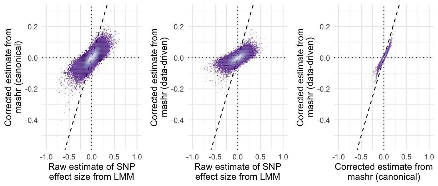
Figure SX: Plots comparing the raw effect sizes for each locus (calculated by linear mixed models implemented in GEMMA, LMM) with the effect sizes obtained using adaptive shrinkage implemented in mashr (either in ‘data-driven’ or ‘canonical’ methods). The dashed line shows \(y = x\), such that the first two plots illustrate that both forms of shrinkage moved both negative and positive effects towards zero. The third plot illustrates that very similar effect sizes were obtained whether we used the data-driven or canonical method.
sessionInfo()R version 4.0.3 (2020-10-10)
Platform: x86_64-apple-darwin17.0 (64-bit)
Running under: macOS Catalina 10.15.7
Matrix products: default
BLAS: /Library/Frameworks/R.framework/Versions/4.0/Resources/lib/libRblas.dylib
LAPACK: /Library/Frameworks/R.framework/Versions/4.0/Resources/lib/libRlapack.dylib
locale:
[1] en_GB.UTF-8/en_GB.UTF-8/en_GB.UTF-8/C/en_GB.UTF-8/en_GB.UTF-8
attached base packages:
[1] stats graphics grDevices utils datasets methods base
other attached packages:
[1] gridExtra_2.3 kableExtra_1.3.4 glue_1.4.2 mashr_0.2.38
[5] ashr_2.2-47 forcats_0.5.0 stringr_1.4.0 dplyr_1.0.0
[9] purrr_0.3.4 readr_2.0.0 tidyr_1.1.0 tibble_3.0.1
[13] ggplot2_3.3.2 tidyverse_1.3.0 workflowr_1.6.2
loaded via a namespace (and not attached):
[1] nlme_3.1-149 fs_1.4.1 bit64_0.9-7 lubridate_1.7.10
[5] RColorBrewer_1.1-2 webshot_0.5.2 httr_1.4.1 rprojroot_1.3-2
[9] tools_4.0.3 backports_1.1.7 R6_2.4.1 irlba_2.3.3
[13] DBI_1.1.0 colorspace_1.4-1 rmeta_3.0 withr_2.2.0
[17] tidyselect_1.1.0 bit_1.1-15.2 compiler_4.0.3 git2r_0.27.1
[21] cli_2.0.2 rvest_0.3.5 xml2_1.3.2 labeling_0.3
[25] scales_1.1.1 hexbin_1.28.1 SQUAREM_2020.2 mvtnorm_1.1-0
[29] mixsqp_0.3-43 systemfonts_0.2.2 digest_0.6.25 rmarkdown_2.5
[33] svglite_1.2.3 pkgconfig_2.0.3 htmltools_0.5.0 dbplyr_1.4.4
[37] invgamma_1.1 highr_0.8 rlang_0.4.6 readxl_1.3.1
[41] RSQLite_2.2.0 rstudioapi_0.11 farver_2.0.3 generics_0.0.2
[45] jsonlite_1.7.0 vroom_1.5.3 magrittr_2.0.1 Matrix_1.2-18
[49] Rcpp_1.0.4.6 munsell_0.5.0 fansi_0.4.1 abind_1.4-5
[53] gdtools_0.2.2 lifecycle_0.2.0 stringi_1.5.3 whisker_0.4
[57] yaml_2.2.1 plyr_1.8.6 grid_4.0.3 blob_1.2.1
[61] parallel_4.0.3 promises_1.1.0 crayon_1.3.4 lattice_0.20-41
[65] haven_2.3.1 hms_0.5.3 knitr_1.32 pillar_1.4.4
[69] reprex_0.3.0 evaluate_0.14 modelr_0.1.8 vctrs_0.3.0
[73] tzdb_0.1.2 httpuv_1.5.3.1 cellranger_1.1.0 gtable_0.3.0
[77] assertthat_0.2.1 xfun_0.22 broom_0.5.6 later_1.0.0
[81] viridisLite_0.3.0 truncnorm_1.0-8 memoise_1.1.0 ellipsis_0.3.1