Plotting the effect sizes after adjustment using mashr
Last updated: 2021-03-04
Checks: 7 0
Knit directory: fitnessGWAS/
This reproducible R Markdown analysis was created with workflowr (version 1.6.2). The Checks tab describes the reproducibility checks that were applied when the results were created. The Past versions tab lists the development history.
Great! Since the R Markdown file has been committed to the Git repository, you know the exact version of the code that produced these results.
Great job! The global environment was empty. Objects defined in the global environment can affect the analysis in your R Markdown file in unknown ways. For reproduciblity it’s best to always run the code in an empty environment.
The command set.seed(20180914) was run prior to running the code in the R Markdown file. Setting a seed ensures that any results that rely on randomness, e.g. subsampling or permutations, are reproducible.
Great job! Recording the operating system, R version, and package versions is critical for reproducibility.
Nice! There were no cached chunks for this analysis, so you can be confident that you successfully produced the results during this run.
Great job! Using relative paths to the files within your workflowr project makes it easier to run your code on other machines.
Great! You are using Git for version control. Tracking code development and connecting the code version to the results is critical for reproducibility.
The results in this page were generated with repository version c606d3d. See the Past versions tab to see a history of the changes made to the R Markdown and HTML files.
Note that you need to be careful to ensure that all relevant files for the analysis have been committed to Git prior to generating the results (you can use wflow_publish or wflow_git_commit). workflowr only checks the R Markdown file, but you know if there are other scripts or data files that it depends on. Below is the status of the Git repository when the results were generated:
Ignored files:
    Ignored:    .DS_Store
    Ignored:    .Rapp.history
    Ignored:    .Rhistory
    Ignored:    .Rproj.user/
    Ignored:    .httr-oauth
    Ignored:    .pversion
    Ignored:    analysis/.DS_Store
    Ignored:    analysis/correlations_SNP_effects_cache/
    Ignored:    analysis/plot_models_variant_effects_cache/
    Ignored:    code/.DS_Store
    Ignored:    code/Drosophila_GWAS.Rmd
    Ignored:    data/.DS_Store
    Ignored:    data/derived/
    Ignored:    data/input/.DS_Store
    Ignored:    data/input/.pversion
    Ignored:    data/input/dgrp.fb557.annot.txt
    Ignored:    data/input/dgrp2.bed
    Ignored:    data/input/dgrp2.bim
    Ignored:    data/input/dgrp2.fam
    Ignored:    data/input/huang_transcriptome/
    Ignored:    figures/.DS_Store

Untracked files:
    Untracked:  Rplots.pdf
    Untracked:  analysis/GO_KEGG_enrichment.Rmd
    Untracked:  analysis/TWAS_tables.Rmd
    Untracked:  code/GO_and_KEGG_gsea.R
    Untracked:  code/eQTL_analysis.Rmd
    Untracked:  code/make_sites_files_for_ARGweaver.R
    Untracked:  code/plotting_results.Rmd
    Untracked:  code/run_argweaver.R
    Untracked:  code/run_mashr.R
    Untracked:  data/argweaver/
    Untracked:  data/input/TF_binding_sites.csv
    Untracked:  figures/GWAS_mixture_proportions.rds
    Untracked:  figures/GWAS_stats_figure.pdf
    Untracked:  figures/TWAS_mixture_proportions.rds
    Untracked:  figures/TWAS_stats_figure.pdf
    Untracked:  figures/antagonism_ratios.pdf
    Untracked:  figures/composite_mixture_figure.pdf
    Untracked:  figures/eff_size_histos.pdf
    Untracked:  figures/stats_figure.pdf
    Untracked:  manuscript/

Unstaged changes:
    Modified:   .gitignore
    Modified:   README.md
    Modified:   analysis/GWAS_tables.Rmd
    Modified:   analysis/TWAS.Rmd
    Modified:   analysis/_site.yml
    Deleted:    analysis/about.Rmd
    Deleted:    analysis/eQTL_analysis.Rmd
    Modified:   analysis/gwas_adaptive_shrinkage.Rmd
    Modified:   analysis/license.Rmd
    Modified:   analysis/make_annotation_database.Rmd
    Modified:   analysis/plot_line_means.Rmd
    Modified:   analysis/plotting_results.Rmd
    Deleted:    code/gwas_adaptive_shrinkage.R
    Modified:   data/input/female_fitness.csv
    Modified:   data/input/female_fitness_CLEANED.csv
    Modified:   data/input/male_fitness.csv
    Modified:   data/input/male_fitness_CLEANED.csv
    Modified:   figures/figure1.eps
    Deleted:    figures/figure1.png
    Modified:   figures/figure2.eps
Note that any generated files, e.g. HTML, png, CSS, etc., are not included in this status report because it is ok for generated content to have uncommitted changes.
These are the previous versions of the repository in which changes were made to the R Markdown (analysis/checking_mashr_results.Rmd) and HTML (docs/checking_mashr_results.html) files. If you’ve configured a remote Git repository (see ?wflow_git_remote), click on the hyperlinks in the table below to view the files as they were in that past version.
| File | Version | Author | Date | Message |
|---|---|---|---|---|
| html | 836a780 | lukeholman | 2021-03-04 | Build site. |
| Rmd | 0af3d41 | lukeholman | 2021-03-04 | big first commit 2021 |
| Rmd | 8d54ea5 | Luke Holman | 2018-12-23 | Initial commit |
| html | 8d54ea5 | Luke Holman | 2018-12-23 | Initial commit |
library(dplyr)
library(readr)
library(ggplot2)
library(gridExtra)
library(tidyr)

db <- DBI::dbConnect(RSQLite::SQLite(),
                     "data/derived/annotations.sqlite3")

# Results for all 1,613,615 SNPs, even those that are in 100% LD with others (these are grouped up by the SNP_clump column)
all_snps <- tbl(db, "univariate_lmm_results")

# All SNPs and SNP groups that are in <100% LD with one another (n = 1,207,357)
SNP_clumps <- all_snps %>% select(-SNP) %>% distinct() %>% collect(n=Inf)
Inspecting the effect of adaptive shrinkage on the SNP effect size estimates
The plots reveal that the R package mashr, which implements multivariate adaptive shrinkage, was effective at shrinking the effect size estimates towards zero. The amount of shrinkage applied was slightly stronger when applying mashr using data-driven covariance matrices, as opposed to ‘canonical’ covariance matrices that were selected a priori by us.
hex_plot <- function(x, y, xlab, ylab){
  ggplot(SNP_clumps, aes_string(x, y)) +
    geom_abline(linetype = 2) +
    geom_vline(xintercept = 0, linetype = 3) +
    geom_hline(yintercept = 0, linetype = 3) +
    stat_binhex(bins = 200, colour = "#FFFFFF00") +
    scale_fill_distiller(palette = "Purples") +
    coord_cartesian(xlim = c(-1,1), ylim = c(-0.55, 0.3)) +
    theme_minimal() + xlab(xlab) + ylab(ylab) +
    theme(legend.position = "none")
}
grid.arrange(
  hex_plot("beta_female_early_raw",
           "beta_female_early_mashr_canonical",
           "Raw estimate of SNP effect size from LMM",
           "Corrected estimate from mashr (canonical)"),
  hex_plot("beta_female_early_raw",
           "beta_female_early_mashr_ED",
           "Raw estimate of SNP effect size from LMM",
           "Corrected estimate from mashr (data-driven)"),
  hex_plot("beta_female_early_mashr_canonical",
         "beta_female_early_mashr_ED",
         "Corrected estimate from mashr (canonical)",
         "Corrected estimate from mashr (data-driven)"),
  ncol = 3)
Relationship between raw \(p\)-values and the local false sign rate
The local false sign rate (defined as the probability that a SNP’s true effect is non-zero and has the same sign as the effect size estimate) was positively correlated with the raw p-value, as expected.
Note that the false sign rate is sometimes ‘more significant’ than the \(p\)-value; one likely reason for this is that the local false sign rate (LFSR) uses the information provided by the correlations among SNP effects on our four fitness traits, while the \(p\)-value ignores this information.
A second reason why the LFSR is often higher is that the LFSR was (noisily) estimated using a Markov chain, in a Bayesian model that incorporates priors, while the \(p\)-value is estimated by maximum likelihood (so there is no statistical noise) and comes from a frequentist model lacking priors (or rather, it has a completely flat prior, unlike the mashr analysis).
The LFSR from the canonical and data-driven approaches are pretty much the same, though results from the data-drive mashr analysis are slightly ‘more significant’ on average (shown by the preponderance of points above the line \(y = x\)).
hex_plot2 <- function(p, xlab, ylab){
    p +
    geom_abline(linetype = 2) +
    stat_binhex(bins = 200, colour = "#FFFFFF00") +
    scale_fill_distiller(palette = "Blues") +
    scale_x_continuous(expand = c(0,0)) + scale_y_continuous(expand = c(0,0)) +
    coord_cartesian(xlim = c(0, 8), ylim = c(0, 8)) +
    theme_minimal() + xlab(xlab) + ylab(ylab) +
    theme(legend.position = "none")
}

grid.arrange(
  SNP_clumps %>%
    ggplot(aes(-log10(pvalue_female_early_raw),
               -log10(LFSR_female_early_mashr_canonical))) %>%
    hex_plot2("-log10 p-value from LMM",
              "-log10 local false sign rate (canonical)"),
  SNP_clumps %>%
    ggplot(aes(-log10(pvalue_female_early_raw),
               -log10(LFSR_female_early_mashr_ED))) %>%
    hex_plot2("-log10 p-value from LMM",
              "-log10 local false sign rate (data-driven)"),
  SNP_clumps %>%
    ggplot(aes(-log10(LFSR_female_early_mashr_canonical),
               -log10(LFSR_female_early_mashr_ED))) %>%
    hex_plot2("-log10 local false sign\nrate (canonical)",
              "-log10 local false sign rate (data-driven)"),
  ncol = 3)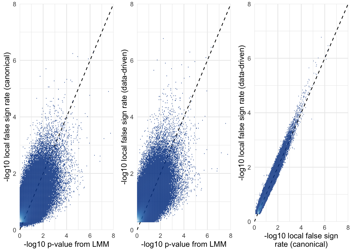
Conclusion
Based on these plots, we elected to focus on the results generated by the data-driven mashr analysis, as opposed to the canonical mashr analysis. This is more conservative, because the effect sizes and local false sign rates are more moderate in the data-driven analysis. Also, using the data-driven approach yields estimates that are independent of our prior expectations about the possible covariance structures that might exist in the data, and is therefore more robust if our expectations are wrong.
sessionInfo()R version 4.0.3 (2020-10-10)
Platform: x86_64-apple-darwin17.0 (64-bit)
Running under: macOS Catalina 10.15.7
Matrix products: default
BLAS: /Library/Frameworks/R.framework/Versions/4.0/Resources/lib/libRblas.dylib
LAPACK: /Library/Frameworks/R.framework/Versions/4.0/Resources/lib/libRlapack.dylib
locale:
[1] en_GB.UTF-8/en_GB.UTF-8/en_GB.UTF-8/C/en_GB.UTF-8/en_GB.UTF-8
attached base packages:
[1] stats graphics grDevices utils datasets methods base
other attached packages:
[1] tidyr_1.1.0 gridExtra_2.3 ggplot2_3.3.2 readr_1.3.1
[5] dplyr_1.0.0 workflowr_1.6.2
loaded via a namespace (and not attached):
[1] Rcpp_1.0.4.6 RColorBrewer_1.1-2 dbplyr_1.4.4 compiler_4.0.3
[5] pillar_1.4.4 later_1.0.0 git2r_0.27.1 tools_4.0.3
[9] bit_1.1-15.2 digest_0.6.25 lattice_0.20-41 memoise_1.1.0
[13] RSQLite_2.2.0 evaluate_0.14 lifecycle_0.2.0 tibble_3.0.1
[17] gtable_0.3.0 pkgconfig_2.0.3 rlang_0.4.6 DBI_1.1.0
[21] yaml_2.2.1 hexbin_1.28.1 xfun_0.19 withr_2.2.0
[25] stringr_1.4.0 knitr_1.30 generics_0.0.2 fs_1.4.1
[29] vctrs_0.3.0 hms_0.5.3 bit64_0.9-7 rprojroot_1.3-2
[33] grid_4.0.3 tidyselect_1.1.0 glue_1.4.2 R6_2.4.1
[37] rmarkdown_2.5 farver_2.0.3 blob_1.2.1 purrr_0.3.4
[41] magrittr_2.0.1 whisker_0.4 backports_1.1.7 scales_1.1.1
[45] promises_1.1.0 htmltools_0.5.0 ellipsis_0.3.1 assertthat_0.2.1
[49] colorspace_1.4-1 httpuv_1.5.3.1 labeling_0.3 stringi_1.5.3
[53] munsell_0.5.0 crayon_1.3.4