Analysis of Experiment 1
Last updated: 2019-10-17
Checks: 7 0
Knit directory: LPS_honeybees/
This reproducible R Markdown analysis was created with workflowr (version 1.4.0). The Checks tab describes the reproducibility checks that were applied when the results were created. The Past versions tab lists the development history.
Great! Since the R Markdown file has been committed to the Git repository, you know the exact version of the code that produced these results.
Great job! The global environment was empty. Objects defined in the global environment can affect the analysis in your R Markdown file in unknown ways. For reproduciblity it’s best to always run the code in an empty environment.
The command set.seed(20190701) was run prior to running the code in the R Markdown file. Setting a seed ensures that any results that rely on randomness, e.g. subsampling or permutations, are reproducible.
Great job! Recording the operating system, R version, and package versions is critical for reproducibility.
Nice! There were no cached chunks for this analysis, so you can be confident that you successfully produced the results during this run.
Great job! Using relative paths to the files within your workflowr project makes it easier to run your code on other machines.
Great! You are using Git for version control. Tracking code development and connecting the code version to the results is critical for reproducibility. The version displayed above was the version of the Git repository at the time these results were generated.
Note that you need to be careful to ensure that all relevant files for the analysis have been committed to Git prior to generating the results (you can use wflow_publish or wflow_git_commit). workflowr only checks the R Markdown file, but you know if there are other scripts or data files that it depends on. Below is the status of the Git repository when the results were generated:
Ignored files:
    Ignored:    .DS_Store
    Ignored:    .Rhistory
    Ignored:    .Rproj.user/
    Ignored:    data/.DS_Store
Note that any generated files, e.g. HTML, png, CSS, etc., are not included in this status report because it is ok for generated content to have uncommitted changes.
These are the previous versions of the R Markdown and HTML files. If you’ve configured a remote Git repository (see ?wflow_git_remote), click on the hyperlinks in the table below to view them.
| File | Version | Author | Date | Message |
|---|---|---|---|---|
| Rmd | 367c1bd | lukeholman | 2019-09-30 | First big commit |
Load data and R packages
library(brms)
library(bayesplot)
library(tidyverse)
library(gridExtra)
library(kableExtra)
library(bayestestR)
library(tidybayes)
source("code/helper_functions.R")

exp2_treatments <- c("Ringer CHC", "LPS CHC")

durations <- read_csv("data/data_collection_sheets/experiment_durations.csv") %>%
  filter(experiment == 2) %>% select(-experiment)

outcome_tally <- read_csv(file = "data/clean_data/experiment_2_outcome_tally.csv") %>%
  mutate(outcome = factor(outcome, levels = c("Stayed inside the hive", "Left of own volition", "Forced out")),
         treatment = factor(treatment, levels = exp2_treatments))

# Re-formatted version of the same data, where each row is an individual bee. We need this format to run the brms model.
data_for_categorical_model <- outcome_tally %>%
  mutate(id = 1:n()) %>%
  split(.$id) %>%
  map(function(x){
    if(x$n[1] == 0) return(NULL)
    data.frame(
      treatment = x$treatment[1],
      hive = x$hive[1],
      colour = x$colour[1],
      outcome = rep(x$outcome[1], x$n))
  }) %>% do.call("rbind", .) %>% as_tibble() %>%
  arrange(hive, treatment) %>%
  mutate(outcome_numeric = as.numeric(outcome),
         hive = as.character(hive),
         treatment = factor(treatment, levels = exp2_treatments)) %>%
  left_join(durations, by = "hive")
Inspect the raw data
Table format
outcome_tally %>%
  kable(digits = 3) %>% kable_styling() %>%
scroll_box(height = "380px")| hive | treatment | colour | outcome | n |
|---|---|---|---|---|
| Arts | LPS CHC | Dark Blue | Stayed inside the hive | 56 |
| Arts | LPS CHC | Dark Blue | Left of own volition | 5 |
| Arts | LPS CHC | Dark Blue | Forced out | 7 |
| Arts | Ringer CHC | Pink | Stayed inside the hive | 64 |
| Arts | Ringer CHC | Pink | Left of own volition | 5 |
| Arts | Ringer CHC | Pink | Forced out | 1 |
| Garden | LPS CHC | Dark Blue | Stayed inside the hive | 70 |
| Garden | LPS CHC | Dark Blue | Left of own volition | 2 |
| Garden | LPS CHC | Dark Blue | Forced out | 3 |
| Garden | Ringer CHC | Pink | Stayed inside the hive | 73 |
| Garden | Ringer CHC | Pink | Left of own volition | 2 |
| Garden | Ringer CHC | Pink | Forced out | 0 |
| Skylab | LPS CHC | Pink | Stayed inside the hive | 93 |
| Skylab | LPS CHC | Pink | Left of own volition | 2 |
| Skylab | LPS CHC | Pink | Forced out | 5 |
| Skylab | Ringer CHC | Dark Blue | Stayed inside the hive | 97 |
| Skylab | Ringer CHC | Dark Blue | Left of own volition | 1 |
| Skylab | Ringer CHC | Dark Blue | Forced out | 1 |
| Zoology | LPS CHC | Pink | Stayed inside the hive | 38 |
| Zoology | LPS CHC | Pink | Left of own volition | 4 |
| Zoology | LPS CHC | Pink | Forced out | 6 |
| Zoology | Ringer CHC | Dark Blue | Stayed inside the hive | 42 |
| Zoology | Ringer CHC | Dark Blue | Left of own volition | 2 |
| Zoology | Ringer CHC | Dark Blue | Forced out | 6 |
Plotted as a bar chart
all_hives <- outcome_tally %>%
  group_by(treatment, outcome) %>%
  summarise(n = sum(n)) %>%
  ungroup() %>% mutate(hive = "All hives")

outcome_tally %>%
  group_by(treatment, hive, outcome) %>%
  summarise(n = sum(n)) %>%
  ungroup() %>%
  mutate(hive = paste(hive, "hive")) %>%
  full_join(all_hives, by = c("treatment", "hive", "outcome", "n")) %>%
  mutate(prop = n / sum(n)) %>%
  ggplot(aes(outcome, n , fill = treatment)) +
  geom_bar(stat = "identity", position = "dodge") +
  facet_wrap( ~ hive, nrow = 1, scales = "free_y") +
  scale_fill_brewer(palette = "Set2", name = "Treatment") +
  xlab("Outcome") + ylab("Number of bees") +
  theme(axis.text.x = element_text(angle = 45, hjust=1))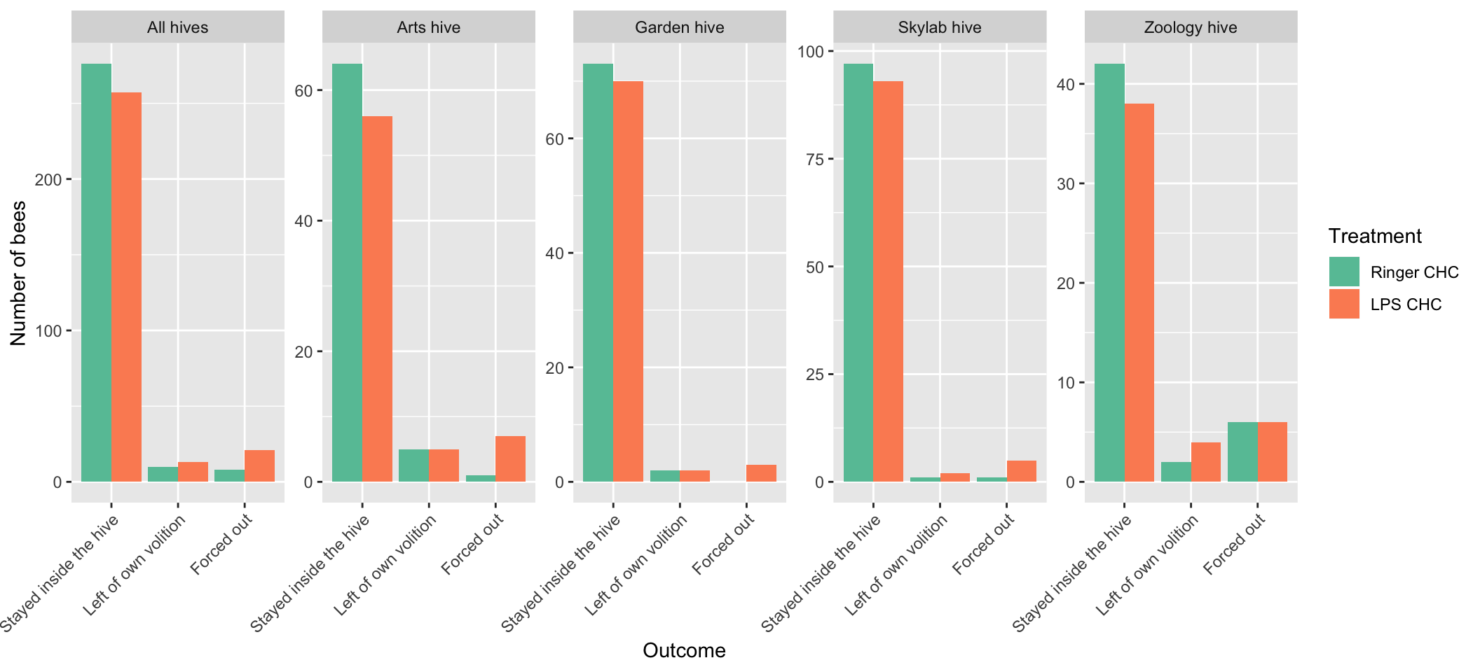
Multinomial model of outcome
Run the models
Fit a multinomial logisitic model, with 3 possible outcomes describing what happened to each bee introduced to the hive: stayed inside, left of its own volition, or forced out by the other workers. To assess the effects of our predictor variables, we compare 5 models with different fixed factors, ranking them by posterior model probability.
if(!file.exists("output/model_probabilities_expt2.rds")){
  my_prior <- c(set_prior("normal(0, 2)", class = "b"))

  run_brms_categorical <- function(formula){
    formula <- gsub(" ", "", paste("outcome_numeric ~", formula))
    brm(formula,
        data = data_for_categorical_model,
        prior = my_prior,
        family = "categorical",
        save_all_pars = TRUE,
        control = list(adapt_delta = 0.999, max_treedepth = 15),
        chains = 4, cores = 4, iter = 40000, seed = 1)
  }

  formula_list <- c(
    "treatment:hive + treatment + hive + observation_time_minutes",
    "treatment + hive + observation_time_minutes",
    "treatment + observation_time_minutes",
    "hive + observation_time_minutes",
    "observation_time_minutes")

  # run all 5 models, sequentially
  model_list_expt2 <- lapply(formula_list, run_brms_categorical)

  # Estimate the log marginal likelihood by bridge sampling, and use to determine the posterior model probabilities
  # See: vignette("bridgesampling_example_stan")
  model_probabilities <- post_prob(model_list_expt2[[1]],
                                   model_list_expt2[[2]],
                                   model_list_expt2[[3]],
                                   model_list_expt2[[4]],
                                   model_list_expt2[[5]])
  top_index <- which.max(unname(model_probabilities))

  model_probabilities <- tibble(
    `Fixed effects` = formula_list,
    `Posterior model probability` = unname(model_probabilities)) %>%
    arrange(-`Posterior model probability`)

  model_probabilities <- model_probabilities %>%
    mutate(`% of top model probability` = round(100 * `Posterior model probability` / `Posterior model probability`[1], 1),
           `% of top model probability` = c("\\-", `% of top model probability`[2:length(`% of top model probability`)]))

 # saveRDS(model_list_expt2[[1]], "output/full_model_expt2.rds")
  saveRDS(model_list_expt2[[top_index]], "output/top_model_expt2.rds")
  saveRDS(model_probabilities, "output/model_probabilities_expt2.rds")
}

top_model <- readRDS("output/top_model_expt2.rds")
model_probabilities <- readRDS("output/model_probabilities_expt2.rds")
Posterior model probabilites
model_probabilities %>%
kable(digits = 3) %>% kable_styling()| Fixed effects | Posterior model probability | % of top model probability |
|---|---|---|
| treatment + observation_time_minutes | 0.566 |
|
| observation_time_minutes | 0.354 | 62.6 |
| treatment + hive + observation_time_minutes | 0.048 | 8.4 |
| hive + observation_time_minutes | 0.027 | 4.8 |
| treatment:hive + treatment + hive + observation_time_minutes | 0.006 | 1 |
Fixed effects from the top model
The model output suggests that the third possible outcome (i.e. being forced out of the hive; denoted as mu3 in the table) was more common in the ‘LPS CHCs’ treatment group. See Hypothesis testing and effect sizes below for more useful statistical results.
get_fixed_effects_with_p_values(top_model) %>%
kable(digits = 3) %>% kable_styling()| Parameter | Estimate | Est.Error | lower_95_CI | upper_95_CI | Rhat | Bulk_ESS | Tail_ESS | p | |
|---|---|---|---|---|---|---|---|---|---|
| mu2_Intercept | -6.396 | 1.191 | -8.931 | -4.262 | 1 | 44785 | 41916 | 0.000 | * |
| mu3_Intercept | -6.002 | 0.993 | -8.059 | -4.176 | 1 | 46424 | 44048 | 0.000 | * |
| mu2_treatmentLPSCHC | 0.362 | 0.431 | -0.474 | 1.223 | 1 | 60598 | 50515 | 0.199 | |
| mu2_observation_time_minutes | 0.030 | 0.011 | 0.011 | 0.052 | 1 | 49351 | 45506 | 0.001 | * |
| mu3_treatmentLPSCHC | 1.054 | 0.422 | 0.261 | 1.914 | 1 | 52801 | 48727 | 0.004 | * |
| mu3_observation_time_minutes | 0.025 | 0.009 | 0.008 | 0.043 | 1 | 53563 | 48343 | 0.001 | * |
Plotting estimates from the model
Derive prediction from the posterior
new <- expand.grid(treatment = levels(data_for_categorical_model$treatment),
                   observation_time_minutes = 120)

preds <- fitted(top_model, newdata = new, summary = FALSE)
dimnames(preds) <- list(NULL, new[,1], NULL)

plotting_data <- rbind(
  as.data.frame(preds[,, 1]) %>% mutate(outcome = "Stayed inside the hive", posterior_sample = 1:n()),
  as.data.frame(preds[,, 2]) %>% mutate(outcome = "Left voluntarily", posterior_sample = 1:n()),
  as.data.frame(preds[,, 3]) %>% mutate(outcome = "Forced out", posterior_sample = 1:n())) %>%
  gather(treatment, prop, `Ringer CHC`, `LPS CHC`) %>%
  mutate(treatment = factor(treatment, c("Ringer CHC", "LPS CHC")),
         outcome = factor(outcome, c("Stayed inside the hive", "Left voluntarily", "Forced out"))) %>%
  as_tibble() %>% arrange(treatment, outcome)
Make Figure 2
ggplot(plotting_data, aes(treatment, 100 * prop)) +
  geom_eye(aes(fill = treatment)) +
  scale_fill_brewer(palette = "Pastel1", direction = -1) +
  facet_wrap( ~ outcome, scales = "free_y") +
  ylab("% bees leaving the hive this way") +
  xlab("Mode of exit") +
  theme_bw() +
theme(legend.position = "none") 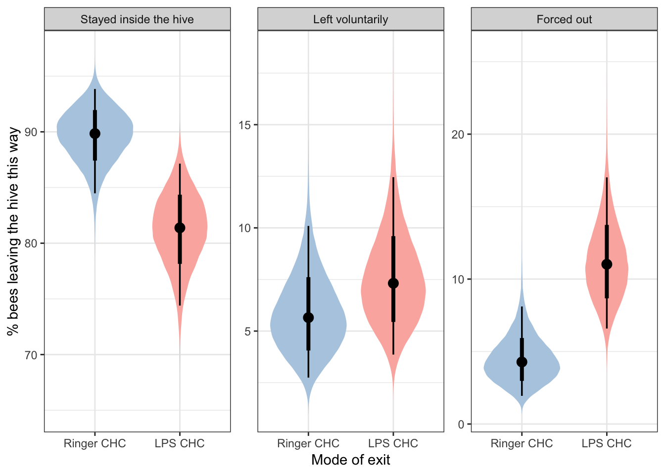
Hypothesis testing and effect sizes
This section calculates the posterior difference in treatment group means, in order to perform some null hypothesis testing, calculate effect size, and calculate the 95% credible intervals on the effect size. In all cases, the effect size expresses the effect of the “LPS-treated bee CHCs” treatment relative to the “Ringer-treated bee CHCs” control.
% bees exiting the hive
my_summary <- function(df, columns, outcome) {
  lapply(columns, function(x){

    p <- df %>% pull(!! x) %>% bayestestR::p_direction() %>% as.numeric()
    p <- (100 - p) / 100

    df %>% pull(!! x) %>% posterior_summary() %>% as_tibble() %>%
      mutate(p=p, Outcome = outcome, Metric = x) %>% select(Outcome, Metric, everything())
  }) %>% do.call("rbind", .)
}

stats_table <- rbind(
  plotting_data %>%
    filter(outcome == "Stayed inside the hive") %>%
    mutate(prop = 1 - prop) %>%
    spread(treatment, prop) %>%
    mutate(`Absolute difference in % bees exiting the hive` = 100 * (`LPS CHC` - `Ringer CHC`),
           `Log10 odds ratio` = log10(`LPS CHC` / `Ringer CHC`)) %>%
    my_summary(c("Absolute difference in % bees exiting the hive",
                 "Log10 odds ratio"),
               outcome = "Stayed inside the hive") %>%
    mutate(p = c(" ", format(round(p[2], 4), nsmall = 4))),

  plotting_data %>%
    filter(outcome == "Left voluntarily") %>%
    spread(treatment, prop) %>%
    mutate(`Absolute difference in % bees leaving voluntarily` = 100 * (`LPS CHC` - `Ringer CHC`),
           `Log10 odds ratio` = log10(`LPS CHC` / `Ringer CHC`)) %>%
    my_summary(c("Absolute difference in % bees leaving voluntarily",
                 "Log10 odds ratio"),
               outcome = "Left voluntarily") %>%
    mutate(p = c(" ", format(round(p[2], 4), nsmall = 4))),

  plotting_data %>%
    filter(outcome == "Forced out") %>%
    spread(treatment, prop) %>%
    mutate(`Absolute difference in % bees leaving voluntarily` = 100 * (`LPS CHC` - `Ringer CHC`),
           `Log10 odds ratio` = log10(`LPS CHC` / `Ringer CHC`)) %>%
    my_summary(c("Absolute difference in % bees leaving voluntarily",
                 "Log10 odds ratio"),
               outcome = "Forced out") %>%
    mutate(p = c(" ", format(round(p[2], 4), nsmall = 4)))
)

stats_table[c(2,4,6), 1] <- " "

stats_table %>%
  mutate(` ` = ifelse(p < 0.05, "\\*", ""),
         ` ` = replace(` `, p < 0.01, "**"),
         ` ` = replace(` `, p < 0.001, "***"),
         ` ` = replace(` `, p == " ", "")) %>%
  kable(digits = 3) %>% kable_styling() %>%
row_spec(c(0,2,4,6), extra_css = "border-bottom: solid;")| Outcome | Metric | Estimate | Est.Error | Q2.5 | Q97.5 | p | |
|---|---|---|---|---|---|---|---|
| Stayed inside the hive | Absolute difference in % bees exiting the hive | 8.437 | 3.649 | 1.456 | 15.812 | ||
| Log10 odds ratio | 0.265 | 0.115 | 0.045 | 0.496 | 0.0092 | ** | |
| Left voluntarily | Absolute difference in % bees leaving voluntarily | 1.685 | 2.639 | -3.397 | 7.087 | ||
| Log10 odds ratio | 0.114 | 0.175 | -0.226 | 0.465 | 0.2559 | ||
| Forced out | Absolute difference in % bees leaving voluntarily | 6.751 | 2.831 | 1.574 | 12.657 | ||
| Log10 odds ratio | 0.415 | 0.172 | 0.094 | 0.768 | 0.0054 | ** |
sessionInfo()R version 3.5.1 (2018-07-02)
Platform: x86_64-apple-darwin15.6.0 (64-bit)
Running under: macOS High Sierra 10.13.6
Matrix products: default
BLAS: /Library/Frameworks/R.framework/Versions/3.5/Resources/lib/libRblas.0.dylib
LAPACK: /Library/Frameworks/R.framework/Versions/3.5/Resources/lib/libRlapack.dylib
locale:
[1] en_AU.UTF-8/en_AU.UTF-8/en_AU.UTF-8/C/en_AU.UTF-8/en_AU.UTF-8
attached base packages:
[1] stats graphics grDevices utils datasets methods base
other attached packages:
[1] tidybayes_1.1.0 bayestestR_0.2.2 kableExtra_0.9.0 gridExtra_2.3
[5] forcats_0.4.0 stringr_1.4.0 dplyr_0.8.3 purrr_0.3.2
[9] readr_1.1.1 tidyr_0.8.2 tibble_2.1.3 ggplot2_3.1.0
[13] tidyverse_1.2.1 bayesplot_1.6.0 brms_2.10.0 Rcpp_1.0.2
loaded via a namespace (and not attached):
[1] colorspace_1.3-2 ggridges_0.5.0
[3] rsconnect_0.8.8 rprojroot_1.3-2
[5] ggstance_0.3.1 markdown_1.0
[7] base64enc_0.1-3 fs_1.3.1
[9] rstudioapi_0.10 rstan_2.19.2
[11] svUnit_0.7-12 DT_0.4
[13] mvtnorm_1.0-11 lubridate_1.7.4
[15] xml2_1.2.0 bridgesampling_0.4-0
[17] knitr_1.23 shinythemes_1.1.1
[19] jsonlite_1.6 workflowr_1.4.0
[21] broom_0.5.0 shiny_1.3.2
[23] compiler_3.5.1 httr_1.4.0
[25] backports_1.1.2 assertthat_0.2.1
[27] Matrix_1.2-14 lazyeval_0.2.2
[29] cli_1.1.0 later_0.8.0
[31] htmltools_0.3.6 prettyunits_1.0.2
[33] tools_3.5.1 igraph_1.2.1
[35] coda_0.19-2 gtable_0.2.0
[37] glue_1.3.1.9000 reshape2_1.4.3
[39] cellranger_1.1.0 nlme_3.1-137
[41] crosstalk_1.0.0 insight_0.3.0
[43] xfun_0.8 ps_1.3.0
[45] rvest_0.3.2 mime_0.7
[47] miniUI_0.1.1.1 gtools_3.8.1
[49] zoo_1.8-3 scales_1.0.0
[51] colourpicker_1.0 hms_0.4.2
[53] promises_1.0.1 Brobdingnag_1.2-5
[55] parallel_3.5.1 inline_0.3.15
[57] shinystan_2.5.0 RColorBrewer_1.1-2
[59] yaml_2.2.0 loo_2.1.0
[61] StanHeaders_2.19.0 stringi_1.4.3
[63] highr_0.8 dygraphs_1.1.1.6
[65] pkgbuild_1.0.2 rlang_0.4.0
[67] pkgconfig_2.0.2 matrixStats_0.54.0
[69] evaluate_0.14 lattice_0.20-35
[71] rstantools_2.0.0 htmlwidgets_1.3
[73] labeling_0.3 processx_3.2.1
[75] tidyselect_0.2.5 plyr_1.8.4
[77] magrittr_1.5 R6_2.4.0
[79] pillar_1.3.1.9000 haven_1.1.2
[81] whisker_0.3-2 withr_2.1.2
[83] xts_0.11-0 abind_1.4-5
[85] modelr_0.1.2 crayon_1.3.4
[87] arrayhelpers_1.0-20160527 rmarkdown_1.13
[89] grid_3.5.1 readxl_1.1.0
[91] callr_2.0.4 git2r_0.23.0
[93] threejs_0.3.1 digest_0.6.20
[95] xtable_1.8-4 httpuv_1.5.1
[97] stats4_3.5.1 munsell_0.5.0
[99] viridisLite_0.3.0 shinyjs_1.0