Modelling G\(\times\)E effects on consumer-resource interactions
Matt Barbour
2020-10-15
Last updated: 2020-10-15
Checks: 7 0
Knit directory: foodweb-theory/
This reproducible R Markdown analysis was created with workflowr (version 1.6.0). The Checks tab describes the reproducibility checks that were applied when the results were created. The Past versions tab lists the development history.
Great! Since the R Markdown file has been committed to the Git repository, you know the exact version of the code that produced these results.
Great job! The global environment was empty. Objects defined in the global environment can affect the analysis in your R Markdown file in unknown ways. For reproduciblity it’s best to always run the code in an empty environment.
The command set.seed(20200205) was run prior to running the code in the R Markdown file. Setting a seed ensures that any results that rely on randomness, e.g. subsampling or permutations, are reproducible.
Great job! Recording the operating system, R version, and package versions is critical for reproducibility.
Nice! There were no cached chunks for this analysis, so you can be confident that you successfully produced the results during this run.
Great job! Using relative paths to the files within your workflowr project makes it easier to run your code on other machines.
Great! You are using Git for version control. Tracking code development and connecting the code version to the results is critical for reproducibility. The version displayed above was the version of the Git repository at the time these results were generated.
Note that you need to be careful to ensure that all relevant files for the analysis have been committed to Git prior to generating the results (you can use wflow_publish or wflow_git_commit). workflowr only checks the R Markdown file, but you know if there are other scripts or data files that it depends on. Below is the status of the Git repository when the results were generated:
Ignored files:
    Ignored:    .Rhistory
    Ignored:    .Rproj.user/

Untracked files:
    Untracked:  Box-3-plot.pdf
    Untracked:  Box-3-plot.png
    Untracked:  analysis/rosenzweig-macarthur.Rmd
    Untracked:  code/Models.R
    Untracked:  rosenzweig-macarthur.png
    Untracked:  temp/

Unstaged changes:
    Modified:   analysis/index.Rmd
    Modified:   analysis/references.bib
    Deleted:    analysis/temperature-dependence.Rmd
Note that any generated files, e.g. HTML, png, CSS, etc., are not included in this status report because it is ok for generated content to have uncommitted changes.
These are the previous versions of the R Markdown and HTML files. If you’ve configured a remote Git repository (see ?wflow_git_remote), click on the hyperlinks in the table below to view them.
| File | Version | Author | Date | Message |
|---|---|---|---|---|
| Rmd | d19252f | mabarbour | 2020-10-15 | GxE analysis of temperature. |
Consumer-resource model
I analyze a continuous time model of a consumer-resource interaction. The resource exhibits logistic growth and the consumer has a type 1 functional response:
\[\frac{dR}{dt}=R(r-\frac{rR}{K}-aC)\] \[\frac{dC}{dt}=C(eaR-m)\]
The following ecological rates govern the dynamics of this model:
r = intrinsic growth rate of resource at low densities
K = carrying capacity of resource
a = attack rate of consumer on the resource
e = conversion efficiency of resources into consumers
m = mortality rate of consumer
I consider these ecological rates as the phenotypes of the consumer and resource. For my initial exploration, I’m going to keep things simple and focus on G\(\times\)E effects of consumers, but I also model the effects of E on resources. I’m also going to link phenotypic change to selection, fitness, and stability.
Following the framework of Gilbert et al. (2014), I assume that the temperature dependence of consumer and resource phenotypes can be modelled as Boltzmann-Arrhenius equations. I focus here on temperature because of its well known influence on consumer and resource phenotypes, and its predictable response to climate change. I also use the biological plausible parameter values that Gilbert et al. (2014) provide in Table 1 and Figure 3 of their paper. I explore the effects of temperature across a gradient from 5-30\(^\circ\)C.
Scaling G\(\times\)E to consumer phenotype
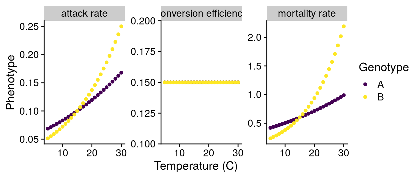
To get a sense for how genotype-by-environment interactions (G\(\times\)E) in consumers might alter these dynamics, I created two different genotypes (A and B). These genotypes have the same “initial” phenotype, which I setup at 15\(^\circ\)C. This choice of temperature was arbitrary and I chose it to follow Fig. 3 of Gilbert et al. (2014). I would argue this represents the effect of genotype (G) as it affects the “intercept” of the phenotype. To simulate a G\(\times\)E effect, I adjusted the activation energy of the temperature relationship (i.e., the slope) assuming a linear tradeoff between genotypes. With these two genotypes, I can visualize G effects (comparing at 15\(^\circ\)C), E effects (mean phenotype change with temperature), and G\(\times\)E effects (different slopes of each genotype).
Scaling G\(\times\)E to consumer attack rate a:
# parameters from Gilbert et al. 2014 and Osmond et al. 2017
E_vC_mean <- 0.46
E_tradeoff <- 0.2
E_vC_A <- E_vC_mean - E_tradeoff
E_vC_B <- E_vC_mean + E_tradeoff

# Genotype A
a_seq <- a_scaling(a0 = a0(a_base = 0.1, v0_C = 1, v0_R = 1,
                           E_vC = E_vC_A, E_vR = 0.46,
                           T_C = C_to_K(15), T_R = C_to_K(15)),
                   v0_C = 1, v0_R = 1, E_vC = E_vC_A, E_vR = 0.46,
                   T_C = C_to_K(Temp_seq), T_R = C_to_K(Temp_seq))

# Genotype B
a_seq2 <- a_scaling(a0 = a0(a_base = 0.1, v0_C = 1, v0_R = 1,
                            E_vC = E_vC_B, E_vR = 0.46,
                            T_C = C_to_K(15), T_R = C_to_K(15)),
                   v0_C = 1, v0_R = 1, E_vC = E_vC_B, E_vR = 0.46,
                   T_C = C_to_K(Temp_seq), T_R = C_to_K(Temp_seq))
Scaling G\(\times\)E to consumer mortality rate m:
E_m_mean <- 0.45
# using same tradeoff
E_m_A <- E_m_mean - E_tradeoff
E_m_B <- E_m_mean + E_tradeoff

m_seq <- m_scaling(m0 = m0(m_base = 0.6, E_m = E_m_A, T = C_to_K(15)),
                   E_m = E_m_A,
                   T = C_to_K(Temp_seq))

m_seq2 <- m_scaling(m0 = m0(m_base = 0.6, E_m = E_m_B, T = C_to_K(15)),
                   E_m = E_m_B,
                   T = C_to_K(Temp_seq))
According to Peters (1983), conversion efficiency e is independent of temperature, so I set e=0.15 as in Fig. 3 of Gilbert et al. (2014).
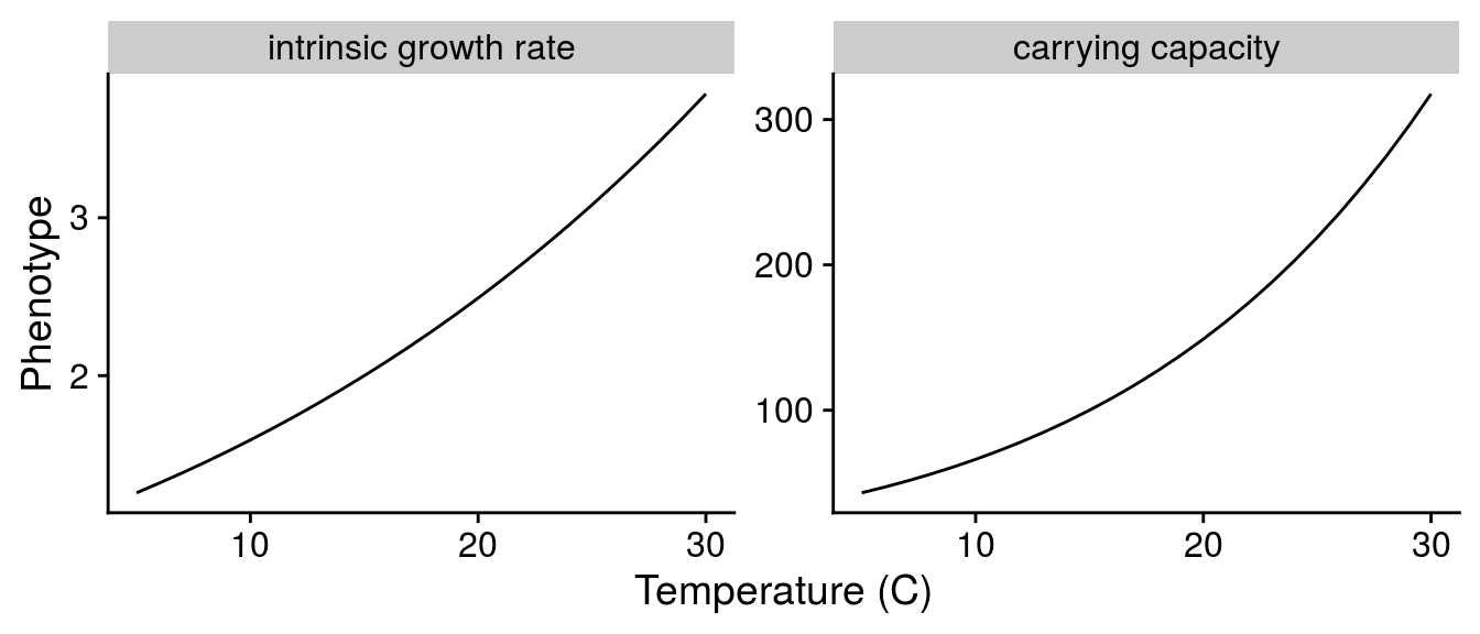
Scaling E to resource phenotype
For resources, I only modelled well known effects of warming.
Scaling intrinsic growth rate r:
# Genotype A
r_seq <- r_scaling(r0 = r0(r_base = 2, E_B = 0.32, T = C_to_K(15)),
                   E_B = 0.32,
                   T = C_to_K(Temp_seq))
Scaling carrying capacity K:
# Genotype A
K_seq <- K_scaling(K0 = K0(K_base = 100, E_B = 0.32, E_S = 0.9, T = C_to_K(15)),
                   E_B = 0.32,
                   E_S = 0.9,
                   T = C_to_K(Temp_seq))
Visualize consumer and resource phenotypes
G\(\times\)E on consumer phenotype
E on resource phenotype
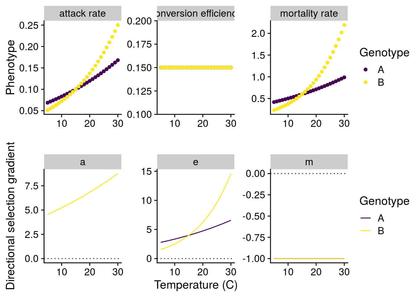
How will G\(\times\)E effects of temperature alter natural selection?
To answer this question, I have to understand how a small change in the phenotype alters the mean fitness (\(\bar{W}\)) of the consumer or resource population (i.e. directional selection). Importantly, both consumer and resource fitness are density-dependent:
\[\bar{W_R}=\frac{1}{R}\frac{dR}{dt}=r-\frac{r}{K}R-aC\] \[\bar{W_C}=\frac{1}{C}\frac{dR}{dt}=eaR-m\]
To make things easier, I assume the consumer and resource dynamics are at an equilibrium and use these values to to estimate selection on each phenotype. Note that I only assess selection acting on the consumer, since I’m primarily interested in the consequences of G\(\times\)E.
Now I can plot both the G\(\times\)E effects of temperature, but also how these G\(\times\)E alters natural selection:
Scaling G\(\times\)E effects to evolutionary change
I’m going to examine how temperature alters the invasion fitness of genotypes A and B. To do this, I need to be able to assess whether Genotype B, e.g., has higher fitness when Genotype A is at equilibrium, and vice versa. But since there phenotypes are different, I need to compare their total phenotype at a particular temperature.
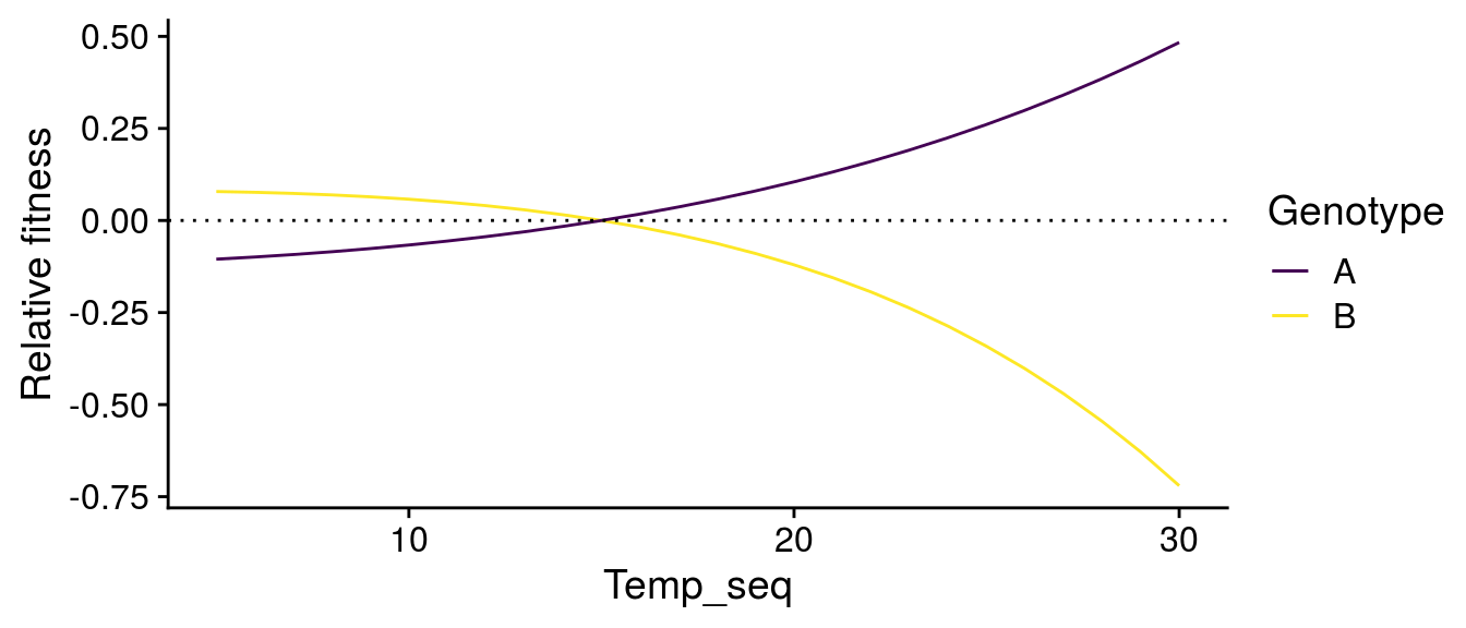
Scaling G\(\times\)E effects to food-web stability
I can also look at how the G\(\times\)E effects of temperature alter the stability of the consumer-resource interactions:
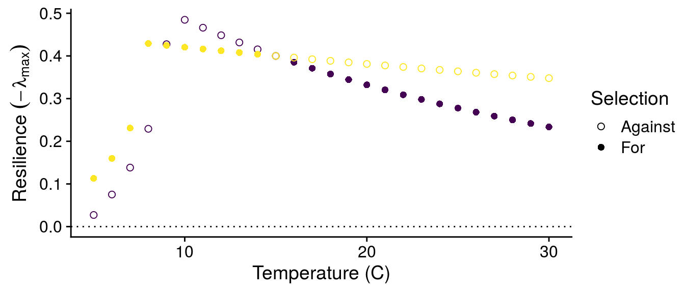
While we still observe a typical stability pattern with temperature (explained in detail in Gilbert et al. 2014), we see that G\(\times\)E effects can switch which genotypes confer greater stability depending on temperature.
Reproduce Fig. 3 in manuscript
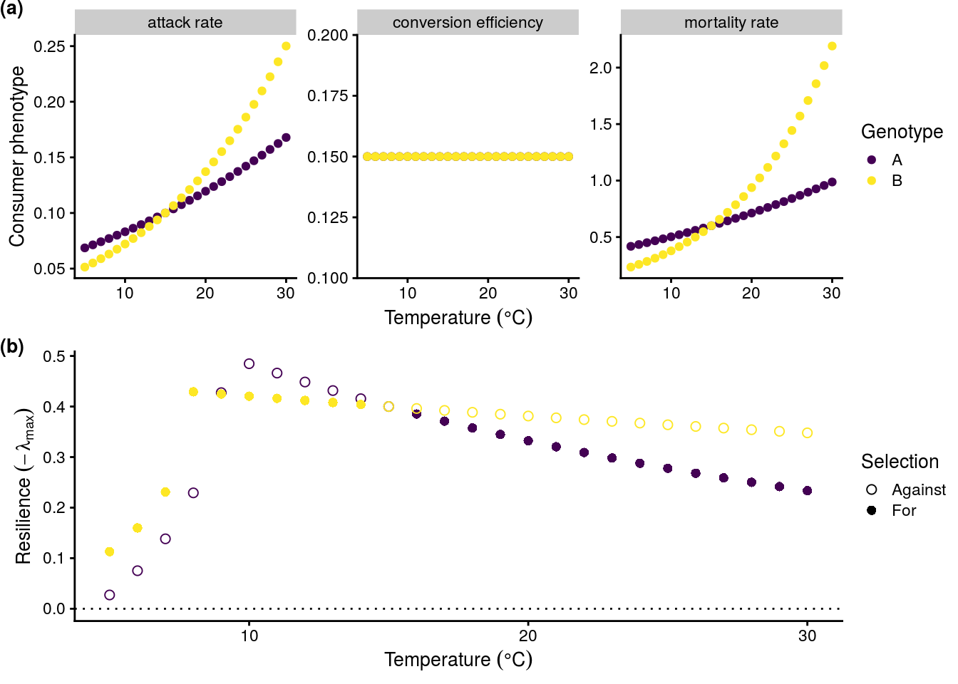
Reproduce Fig. 3 in manuscript.
References
Gilbert, Benjamin, Tyler D Tunney, Kevin S McCann, John P DeLong, David A Vasseur, Van Savage, Jonathan B Shurin, et al. 2014. “A Bioenergetic Framework for the Temperature Dependence of Trophic Interactions.” Ecol. Lett. 17 (8): 902–14.
Peters, Robert Henry. 1983. The Ecological Implications of Body Size. Cambridge University Press.
sessionInfo()R version 3.6.3 (2020-02-29)
Platform: x86_64-pc-linux-gnu (64-bit)
Running under: Ubuntu 16.04.7 LTS
Matrix products: default
BLAS: /usr/lib/libblas/libblas.so.3.6.0
LAPACK: /usr/lib/lapack/liblapack.so.3.6.0
locale:
[1] LC_CTYPE=en_US.UTF-8 LC_NUMERIC=C
[3] LC_TIME=en_US.UTF-8 LC_COLLATE=en_US.UTF-8
[5] LC_MONETARY=en_US.UTF-8 LC_MESSAGES=en_US.UTF-8
[7] LC_PAPER=en_US.UTF-8 LC_NAME=C
[9] LC_ADDRESS=C LC_TELEPHONE=C
[11] LC_MEASUREMENT=en_US.UTF-8 LC_IDENTIFICATION=C
attached base packages:
[1] stats graphics grDevices utils datasets methods base
other attached packages:
[1] cowplot_1.0.0 forcats_0.4.0 stringr_1.4.0 dplyr_0.8.3
[5] purrr_0.3.3 readr_1.3.1 tidyr_1.0.2 tibble_2.1.3
[9] ggplot2_3.2.1 tidyverse_1.3.0 rootSolve_1.7 deSolve_1.24
loaded via a namespace (and not attached):
[1] tidyselect_0.2.5 xfun_0.9 haven_2.2.0 lattice_0.20-38
[5] colorspace_1.4-1 vctrs_0.2.2 generics_0.0.2 viridisLite_0.3.0
[9] htmltools_0.3.6 yaml_2.2.0 rlang_0.4.4 later_1.0.0
[13] pillar_1.4.2 withr_2.1.2 glue_1.3.1 DBI_1.0.0
[17] dbplyr_1.4.2 modelr_0.1.5 readxl_1.3.1 lifecycle_0.1.0
[21] munsell_0.5.0 gtable_0.3.0 workflowr_1.6.0 cellranger_1.1.0
[25] rvest_0.3.5 evaluate_0.14 labeling_0.3 knitr_1.26
[29] httpuv_1.5.1 highr_0.8 broom_0.5.2 Rcpp_1.0.2
[33] promises_1.0.1 backports_1.1.4 scales_1.0.0 jsonlite_1.6
[37] fs_1.3.1 hms_0.5.3 digest_0.6.20 stringi_1.4.3
[41] grid_3.6.3 rprojroot_1.3-2 cli_1.1.0 tools_3.6.3
[45] magrittr_1.5 lazyeval_0.2.2 crayon_1.3.4 whisker_0.3-2
[49] pkgconfig_2.0.2 ellipsis_0.3.0 xml2_1.2.2 reprex_0.3.0
[53] lubridate_1.7.4 rstudioapi_0.10 assertthat_0.2.1 rmarkdown_2.0
[57] httr_1.4.1 R6_2.4.0 nlme_3.1-140 git2r_0.26.1
[61] compiler_3.6.3