Community persistence
Matthew Barbour
2020-10-11
Last updated: 2020-10-11
Checks: 7 0
Knit directory: genes-to-foodweb-stability/
This reproducible R Markdown analysis was created with workflowr (version 1.6.0). The Checks tab describes the reproducibility checks that were applied when the results were created. The Past versions tab lists the development history.
Great! Since the R Markdown file has been committed to the Git repository, you know the exact version of the code that produced these results.
Great job! The global environment was empty. Objects defined in the global environment can affect the analysis in your R Markdown file in unknown ways. For reproduciblity it’s best to always run the code in an empty environment.
The command set.seed(20200205) was run prior to running the code in the R Markdown file. Setting a seed ensures that any results that rely on randomness, e.g. subsampling or permutations, are reproducible.
Great job! Recording the operating system, R version, and package versions is critical for reproducibility.
Nice! There were no cached chunks for this analysis, so you can be confident that you successfully produced the results during this run.
Great job! Using relative paths to the files within your workflowr project makes it easier to run your code on other machines.
Great! You are using Git for version control. Tracking code development and connecting the code version to the results is critical for reproducibility. The version displayed above was the version of the Git repository at the time these results were generated.
Note that you need to be careful to ensure that all relevant files for the analysis have been committed to Git prior to generating the results (you can use wflow_publish or wflow_git_commit). workflowr only checks the R Markdown file, but you know if there are other scripts or data files that it depends on. Below is the status of the Git repository when the results were generated:
Ignored files:
    Ignored:    .Rhistory
    Ignored:    .Rproj.user/
    Ignored:    code/.Rhistory

Untracked files:
    Untracked:  output/community-persistence-keystone.RData
    Untracked:  output/critical-transitions-keystone.RData
    Untracked:  output/structural-stability-keystone.RData

Unstaged changes:
    Modified:   output/plant-growth-no-insects.RData
Note that any generated files, e.g. HTML, png, CSS, etc., are not included in this status report because it is ok for generated content to have uncommitted changes.
These are the previous versions of the R Markdown and HTML files. If you’ve configured a remote Git repository (see ?wflow_git_remote), click on the hyperlinks in the table below to view them.
| File | Version | Author | Date | Message |
|---|---|---|---|---|
| Rmd | 761af40 | mabarbour | 2020-10-11 | Refocus analysis on keystone gene result. |
Setup
# Load and manage data
df <- read_csv("data/arabidopsis_clean_df.csv") %>%
  # renaming for brevity
  rename(cage = Cage,
         com = Composition,
         week = Week,
         temp = Temperature,
         rich = Richness) %>%
  mutate(cage = as.character(cage),
         fweek = factor(ifelse(week < 10, paste("0", week, sep=""), week)),
         temp = ifelse(temp=="20 C", 0, 3)) %>% # set to 3 so that 1 C = 1 genotype
  arrange(cage, week)

# focus on last week of experiment
df17 <- df %>%
  # counter information is not relevant (because it is the same), so we summarise across it
  group_by(cage, fweek, week, temp, rich, Col, gsm1, AOP2, AOP2.gsoh, com) %>%
  summarise_at(vars(BRBR_Survival, LYER_Survival, Mummy_Ptoids_Survival), list(mean)) %>%
  ungroup() %>%
  # we need the dataset to go through week 17, rather than removing cages as they transition
  # to a collapsed community as in `state_df`
  mutate(BRBR = ifelse(is.na(BRBR_Survival) == T, 0, BRBR_Survival),
         LYER = ifelse(is.na(LYER_Survival) == T, 0, LYER_Survival),
         Ptoid = ifelse(is.na(Mummy_Ptoids_Survival) == T, 0, Mummy_Ptoids_Survival)) %>%
  filter(week == 17) %>%
  mutate(# calculate persistence
    Persistence = BRBR + LYER + Ptoid,
    rich - 1, # baseline of 1 genotype
    # define orthogonal constrasts to test for above-average allele effects.
    # aop2_vs_AOP2 must be included first before testing for mam1_vs_MAM1 and gsoh_vs_GSOH
    aop2_vs_AOP2 = Col + gsm1 - AOP2 - AOP2.gsoh,
    mam1_vs_MAM1 = gsm1 - Col,
    gsoh_vs_GSOH = AOP2.gsoh - AOP2)
# note that lowercase denotes the null (non-functional) version of the allele
# wherease capital indicates the functional form
# source in useful functions for analyses
source('code/glm-ftest.R') # ANOVA GLMAnalysis
Below, we reproduce the analysis of deviance for food-web persistence presented in Table S1 in the Supplementary Material.
The analysis below tests for a general effect of genetic diversity (rich) as well as above-average effects of allelic differences at AOP2, MAM1, and GSOH. It also tests for an effect of temperature (temp) and whether temperature modifies any of these genetic effects.
glm.ftest.v2(
  model = glm(data = df17,
              family = quasibinomial(link = "cloglog"),
              formula = terms(Persistence/3 ~
                                temp + rich + aop2_vs_AOP2 + mam1_vs_MAM1 + gsoh_vs_GSOH + com +
                                temp:(rich + aop2_vs_AOP2 + mam1_vs_MAM1 + gsoh_vs_GSOH) + temp:com,
                              keep.order = T)),
  test.formula = list(
    c("temp","temp:com"),
    c("rich","com"),
    c("aop2_vs_AOP2","com"),
    c("mam1_vs_MAM1","com"),
    c("gsoh_vs_GSOH","com"),
    c("temp:rich","temp:com"),
    c("temp:aop2_vs_AOP2","temp:com"),
    c("temp:mam1_vs_MAM1","temp:com"),
    c("temp:gsoh_vs_GSOH","temp:com"))
)[[3]] %>%
  select(Source = treatment,
         `df (Source)` = num_df,
         `df (Error)` = den_df,
         Deviance = deviance,
         `Mean Deviance` = mean_deviance,
         F = F, P = P, Error = error)
Source df (Source) df (Error) Deviance Mean Deviance F P
1 temp 1 6 1.87 1.87 3.294 0.119
2 rich 1 6 1.32 1.32 20.153 0.004
3 aop2_vs_AOP2 1 6 0.75 0.75 11.499 0.015
4 mam1_vs_MAM1 1 6 0.00 0.00 0.008 0.931
5 gsoh_vs_GSOH 1 6 0.08 0.08 1.236 0.309
6 temp:rich 1 6 0.02 0.02 0.028 0.873
7 temp:aop2_vs_AOP2 1 6 0.03 0.03 0.046 0.837
8 temp:mam1_vs_MAM1 1 6 0.40 0.40 0.698 0.435
9 temp:gsoh_vs_GSOH 1 6 0.19 0.19 0.329 0.587
Error
1 temp:com
2 com
3 com
4 com
5 com
6 temp:com
7 temp:com
8 temp:com
9 temp:comWe observe a clear effect of genetic diversity and an above-average contribution of AOP2 to food-web persistence. Temperature did not have a clear effect on food-web persistence and didn’t modify genetic effects.
Effect sizes
Genetic diversity increased the probability of a species persisting by 0.3911896%.
# calculate change in probability
exp(coef(glm(data = df17, family = quasibinomial(link = "cloglog"), formula = Persistence/3 ~ temp + rich))["rich"]) - 1
rich
0.3911896 Keystone gene plot (Fig. 1 in main text)
gene_CI <- conf_int(
  glm(data = df17,
      family = quasibinomial(link = "cloglog"),
      formula = terms(Persistence/3 ~
                        temp + rich + aop2_vs_AOP2 + mam1_vs_MAM1 + gsoh_vs_GSOH,
                      keep.order = T)),
  vcov = "CR2",
  test = "naive-t",
  cluster = df17$com,
  coefs = c("aop2_vs_AOP2","mam1_vs_MAM1","gsoh_vs_GSOH")
) %>%
  data.frame() %>%
  rownames_to_column(var = "term") %>%
  mutate(gene = factor(c("AOP2","MAM1","GSOH"), levels = c("AOP2","MAM1","GSOH")))#ordered = T))

# replacing the average genotype with a genotype that has an aop2 (vs AOP2) allele
# results in a 28% increase in probability of a species persisting
exp(gene_CI$beta[1])-1
[1] 0.2824477# this plot makes clear that AOP2 gene has an above-average effect on community persistence.
ggplot(gene_CI, aes(x = gene, y = exp(beta)-1)) +
geom_point(size = 5) +
geom_linerange(aes(ymax = exp(beta + SE)-1, ymin = exp(beta - SE)-1), size = 1.5) +
geom_linerange(aes(ymax = exp(CI_U)-1, ymin = exp(CI_L)-1)) +
geom_hline(yintercept = 0, linetype = "dotted") +
scale_x_discrete(labels = c(expression(italic(AOP2)),expression(italic(MAM1)),expression(italic(GSOH)))) +
#scale_y_continuous("Probability of species persisting ()") +
scale_y_continuous(name = expression("Effect on food-web persistence "(Delta~"%"))) + # "odds"
xlab("")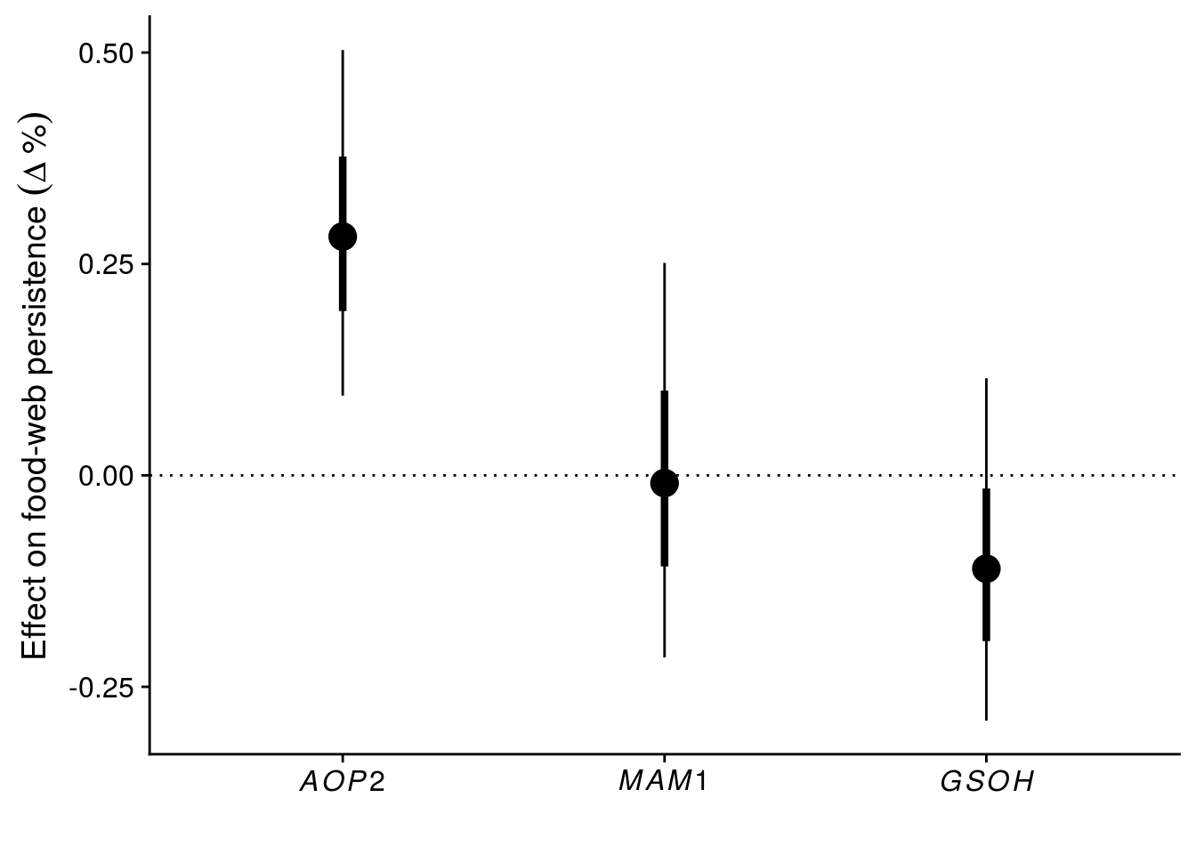
# ggsave(filename = "figures/keystone-gene.pdf", height = 6, width = 8)Let’s visualize the effect of particular alleles within AOP2.
aop2_CI <- conf_int(
  glm(data = df17,
      family = quasibinomial(link = "cloglog"),
      formula = terms(Persistence/3 ~
                        temp + I(AOP2 + AOP2.gsoh) + I(Col + gsm1),
                      keep.order = T)),
  vcov = "CR2",
  test = "naive-t",
  cluster = df17$com,
  coefs = c("I(AOP2 + AOP2.gsoh)","I(Col + gsm1)")
) %>%
  data.frame() %>%
  rownames_to_column(var = "term") %>%
  mutate(allele = c("AOP2","aop2"))
exp(aop2_CI$beta[2])-1 # 80% increase
[1] 0.7992812# get the effect of each genotype
mean_geno <- conf_int(
glm(data = df17,
family = quasibinomial(link = "cloglog"),
formula = terms(Persistence/3 ~
temp + AOP2 + AOP2.gsoh + Col + gsm1,
keep.order = T)),
vcov = "CR2",
test = "naive-t",
cluster = df17$com,
coefs = c("AOP2","AOP2.gsoh","Col","gsm1")
) %>%
data.frame() %>%
rownames_to_column(var = "term") %>%
mutate(allele = c("AOP2","AOP2","aop2","aop2"),
term = factor(term, levels = c("Col","gsm1","AOP2","AOP2.gsoh"), labels = c("Col","gsm1","AOP2","AOP2/gsoh")))
# adding a genotype with an aop2 allele to the population doubles the likelihood of species persistence
ggplot(aop2_CI, aes(x = allele, y = exp(beta)-1)) +
geom_point(size = 5) +
geom_point(data = mean_geno, aes(color = term), size = 5, position = position_dodge(width = 0.3)) +
geom_linerange(aes(ymax = exp(beta + SE)-1, ymin = exp(beta - SE)-1), size = 1.5) +
geom_linerange(aes(ymax = exp(CI_U)-1, ymin = exp(CI_L)-1)) +
geom_hline(yintercept = 0, linetype = "dotted") +
scale_x_discrete(labels = c("AOP2\u2013","AOP2+")) +
scale_y_continuous(expression("Effect on food-web persistence "(Delta~"%"))) +
xlab("Allele") + #xlab(expression("Allele at "~italic(AOP2)~"gene")) +
scale_color_manual(values = c("darkgreen","steelblue","darkorange","firebrick1"), name = "")#, name = "Genotype")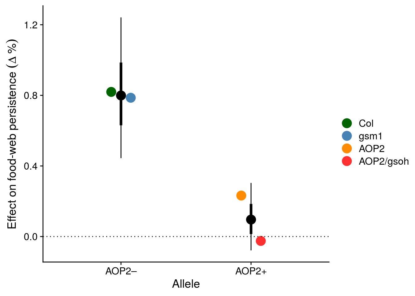
Does AOP2\(-\) explain genetic diversity effect?
glm.ftest.v2(
  model = glm(data = df17,
              family = quasibinomial(link = "cloglog"),
              formula = terms(Persistence/3 ~
                                temp + I(Col + gsm1) + rich + com +
                                temp + temp:com,
                              keep.order = T)),
  test.formula = list(
    c("temp","temp:com"),
    c("I(Col + gsm1)","com"),
    #c("I(AOP2 + AOP2.gsoh)","com"), # rich has a very strong effect if you only include AOP2 + AOP2.gsoh
    c("rich","com"))
)[[3]] %>%
  select(Source = treatment,
         `df (Source)` = num_df,
         `df (Error)` = den_df,
         Deviance = deviance,
         `Mean Deviance` = mean_deviance,
         F = F, P = P, Error = error)
Source df (Source) df (Error) Deviance Mean Deviance F P
1 temp 1 10 1.87 1.87 4.639 0.057
2 I(Col + gsm1) 1 8 2.01 2.01 33.965 <0.001
3 rich 1 8 0.06 0.06 0.988 0.349
Error
1 temp:com
2 com
3 comThe above model suggests that the effect of genetic diversity is explained entirely by the increased probability of having genotypes with an AOP2\(-\) in the plant population.
Note that if instead we modeled the effect of AOP2+ before genetic diversity, we still observe a clear effect of genetic diversity.
glm.ftest.v2(
  model = glm(data = df17,
              family = quasibinomial(link = "cloglog"),
              formula = terms(Persistence/3 ~
                                temp + I(AOP2 + AOP2.gsoh) + rich + com +
                                temp + temp:com,
                              keep.order = T)),
  test.formula = list(
    c("temp","temp:com"),
    #c("I(Col + gsm1)","com"),
    c("I(AOP2 + AOP2.gsoh)","com"),
    c("rich","com"))
)[[3]] %>%
  select(Source = treatment,
         `df (Source)` = num_df,
         `df (Error)` = den_df,
         Deviance = deviance,
         `Mean Deviance` = mean_deviance,
         F = F, P = P, Error = error)
Source df (Source) df (Error) Deviance Mean Deviance F
1 temp 1 10 1.87 1.87 4.639
2 I(AOP2 + AOP2.gsoh) 1 8 0.02 0.02 0.376
3 rich 1 8 2.04 2.04 34.577
P Error
1 0.057 temp:com
2 0.557 com
3 <0.001 comSave analysis
Write out an .RData file to use for creating the Supplementary Material Results.
# save.image(file = "output/community-persistence-keystone.RData")
sessionInfo()R version 3.6.3 (2020-02-29)
Platform: x86_64-pc-linux-gnu (64-bit)
Running under: Ubuntu 16.04.7 LTS
Matrix products: default
BLAS: /usr/lib/libblas/libblas.so.3.6.0
LAPACK: /usr/lib/lapack/liblapack.so.3.6.0
locale:
[1] LC_CTYPE=en_US.UTF-8 LC_NUMERIC=C
[3] LC_TIME=en_US.UTF-8 LC_COLLATE=en_US.UTF-8
[5] LC_MONETARY=en_US.UTF-8 LC_MESSAGES=en_US.UTF-8
[7] LC_PAPER=en_US.UTF-8 LC_NAME=C
[9] LC_ADDRESS=C LC_TELEPHONE=C
[11] LC_MEASUREMENT=en_US.UTF-8 LC_IDENTIFICATION=C
attached base packages:
[1] stats graphics grDevices utils datasets methods base
other attached packages:
[1] kableExtra_1.1.0 clubSandwich_0.3.5 cowplot_1.0.0 forcats_0.4.0
[5] stringr_1.4.0 dplyr_0.8.3 purrr_0.3.3 readr_1.3.1
[9] tidyr_1.0.2 tibble_2.1.3 ggplot2_3.2.1 tidyverse_1.3.0
loaded via a namespace (and not attached):
[1] Rcpp_1.0.2 lubridate_1.7.4 lattice_0.20-38 zoo_1.8-6
[5] assertthat_0.2.1 rprojroot_1.3-2 digest_0.6.20 R6_2.4.0
[9] cellranger_1.1.0 backports_1.1.4 reprex_0.3.0 evaluate_0.14
[13] httr_1.4.1 pillar_1.4.2 rlang_0.4.4 lazyeval_0.2.2
[17] readxl_1.3.1 rstudioapi_0.10 whisker_0.3-2 rmarkdown_2.0
[21] labeling_0.3 webshot_0.5.1 munsell_0.5.0 broom_0.5.2
[25] compiler_3.6.3 httpuv_1.5.1 modelr_0.1.5 xfun_0.9
[29] pkgconfig_2.0.2 htmltools_0.3.6 tidyselect_0.2.5 workflowr_1.6.0
[33] viridisLite_0.3.0 crayon_1.3.4 dbplyr_1.4.2 withr_2.1.2
[37] later_1.0.0 grid_3.6.3 nlme_3.1-140 jsonlite_1.6
[41] gtable_0.3.0 lifecycle_0.1.0 DBI_1.0.0 git2r_0.26.1
[45] magrittr_1.5 scales_1.0.0 cli_1.1.0 stringi_1.4.3
[49] fs_1.3.1 promises_1.0.1 xml2_1.2.2 generics_0.0.2
[53] vctrs_0.2.2 sandwich_2.5-1 tools_3.6.3 glue_1.3.1
[57] hms_0.5.3 yaml_2.2.0 colorspace_1.4-1 rvest_0.3.5
[61] knitr_1.26 haven_2.2.0