Bayesian MAR(1) models and structural stability
Matthew A. Barbour
2020-10-11
Last updated: 2020-10-11
Checks: 7 0
Knit directory: genes-to-foodweb-stability/
This reproducible R Markdown analysis was created with workflowr (version 1.6.0). The Checks tab describes the reproducibility checks that were applied when the results were created. The Past versions tab lists the development history.
Great! Since the R Markdown file has been committed to the Git repository, you know the exact version of the code that produced these results.
Great job! The global environment was empty. Objects defined in the global environment can affect the analysis in your R Markdown file in unknown ways. For reproduciblity it’s best to always run the code in an empty environment.
The command set.seed(20200205) was run prior to running the code in the R Markdown file. Setting a seed ensures that any results that rely on randomness, e.g. subsampling or permutations, are reproducible.
Great job! Recording the operating system, R version, and package versions is critical for reproducibility.
Nice! There were no cached chunks for this analysis, so you can be confident that you successfully produced the results during this run.
Great job! Using relative paths to the files within your workflowr project makes it easier to run your code on other machines.
Great! You are using Git for version control. Tracking code development and connecting the code version to the results is critical for reproducibility. The version displayed above was the version of the Git repository at the time these results were generated.
Note that you need to be careful to ensure that all relevant files for the analysis have been committed to Git prior to generating the results (you can use wflow_publish or wflow_git_commit). workflowr only checks the R Markdown file, but you know if there are other scripts or data files that it depends on. Below is the status of the Git repository when the results were generated:
Ignored files:
    Ignored:    .Rhistory
    Ignored:    .Rproj.user/
    Ignored:    code/.Rhistory

Untracked files:
    Untracked:  output/community-persistence-keystone.RData
    Untracked:  output/critical-transitions-keystone.RData
    Untracked:  output/structural-stability-keystone.RData

Unstaged changes:
    Modified:   output/plant-growth-no-insects.RData
Note that any generated files, e.g. HTML, png, CSS, etc., are not included in this status report because it is ok for generated content to have uncommitted changes.
These are the previous versions of the R Markdown and HTML files. If you’ve configured a remote Git repository (see ?wflow_git_remote), click on the hyperlinks in the table below to view them.
| File | Version | Author | Date | Message |
|---|---|---|---|---|
| Rmd | 761af40 | mabarbour | 2020-10-11 | Refocus analysis on keystone gene result. |
Setup
# load data
timeseries_df <- read_csv("output/timeseries_df.csv") %>%
  mutate(# this makes the intercept correspond to rich = 1, rather
         # than the biologically implausible rich = 0
         rich = rich - 1,
         # now rich and temp coefficients will correspond to +1 genotype and +1 C
         temp = ifelse(temp == "20 C", 0, 3),
         uniq = paste(Cage, temp, com, Week_match, sep = "-"),
         Week_match.1p = 1 + Week_match) # analysis doesn't like initial Week_match = 0, so I just added 1

# filter dataset for multivariate analysis.
# I only retain data for which all species had positive abundances at the previous time step
full_df <- filter(timeseries_df, BRBR_t > 0, LYER_t > 0, Ptoid_t > 0) %>%
  mutate(aop2_genotypes = Col + gsm1, # corresponds to average effect of genotype with a null AOP2- allele
         AOP2_genotypes = AOP2 + AOP2.gsoh) # correspond to average effect of genotype with a functional AOP2+ allele
## source in useful functions
# functions for plotting feasibility domains and calculating normalized angles from critical boundary
source("code/plot-feasibility-domain.R")
# functions for non-equilibrium simulation
source("code/simulate-community-dynamics.R")
# general functions for evaluating what percentage of posterior is aop2 > AOP2 for the LYER-Ptoid boundary. these functions were important for guiding my model selection
source("code/AOP2-LYER-Ptoid-persistence.R")Full model
This model corresponds to equation 1 in the Supplementary Material of the paper. Note that BRBR = aphid Brevicoryne brassicae, LYER = aphid Lipaphis erysimi, and Ptoid = parasitoid Diaeretiella rapae.
# BRBR
full.mv.norm.BRBR.bf <- bf(log1p(BRBR_t1) ~
                       0 + intercept + offset(log1p(BRBR_t)) +
                        (log1p(BRBR_t) + log1p(LYER_t) + log1p(Ptoid_t))*(temp + aop2_genotypes + AOP2_genotypes) +
                        log(Biomass_g_t1) +
                        (1 | Cage) +
                        ar(time = Week_match.1p, gr = Cage, p = 1, cov = FALSE))

# LYER
full.mv.norm.LYER.bf <- bf(log1p(LYER_t1) ~
                       0 + intercept + offset(log1p(LYER_t)) +
                        (log1p(BRBR_t) + log1p(LYER_t) + log1p(Ptoid_t))*(temp + aop2_genotypes + AOP2_genotypes) +
                        log(Biomass_g_t1) +
                        (1 | Cage) +
                        ar(time = Week_match.1p, gr = Cage, p = 1, cov = FALSE))

# Ptoid
full.mv.norm.Ptoid.bf <- bf(log1p(Ptoid_t1) ~
                       0 + intercept + offset(log1p(Ptoid_t)) +
                        (log1p(BRBR_t) + log1p(LYER_t) + log1p(Ptoid_t))*(temp + aop2_genotypes + AOP2_genotypes) +
                        log(Biomass_g_t1) +
                        (1 | Cage) +
                        ar(time = Week_match.1p, gr = Cage, p = 1, cov = FALSE))
Set priors
Intrinsic growth rates
# from Jahan et al. 2014, Journal of Insect Science
# Table 4 lambda (finite rate of increase, discrete time analogue of intrinsic growth rate)
# calculated on a per-day basis and not logged. This is why I multiply by 7 and then take the natural logarithm
Jahan.r.BRBR <- log(c(1.42, 1.36, 1.32, 1.35, 1.40, 1.33, 1.38, 1.37) * 7)
mean(Jahan.r.BRBR) # 2.26
[1] 2.257713sd(Jahan.r.BRBR) # 0.02[1] 0.02468356# visualize prior
hist(rnorm(1000, mean(Jahan.r.BRBR), sd = 1))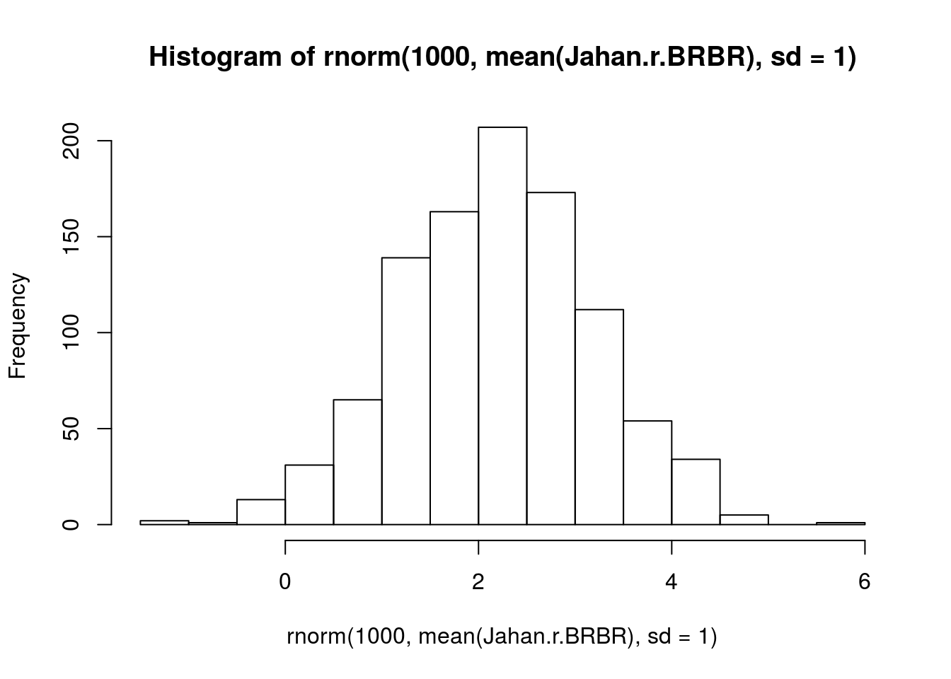
prior.r.BRBR <- "normal(2.26, 1)"

# from Taghizadeh 2019, J. Agr. Sci. Tech.
# Table 2 lambda (finite rate of increase, discrete time analogue of intrinsic growth rate)
# calculated on a per-day basis and not logged. This is why I multiply by 7 and then take the natural logarithm
Tag.r.LYER <- log(c(1.35, 1.30, 1.26, 1.23) * 7)
mean(Tag.r.LYER) # 2.20
[1] 2.196059sd(Tag.r.LYER) # 0.04[1] 0.04028153# visualize prior
hist(rnorm(1000, mean(Tag.r.LYER), sd = 1))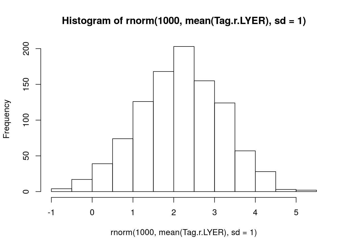
prior.r.LYER <- "normal(2.20, 1)"

# random effects prior based on variance among cultivars
# I'm just going to use this for all of them
mean.r.sd <- mean(c(sd(Jahan.r.BRBR), sd(Tag.r.LYER)))
# visualize prior
hist(rnorm(1000, mean = mean.r.sd, sd = 0.5))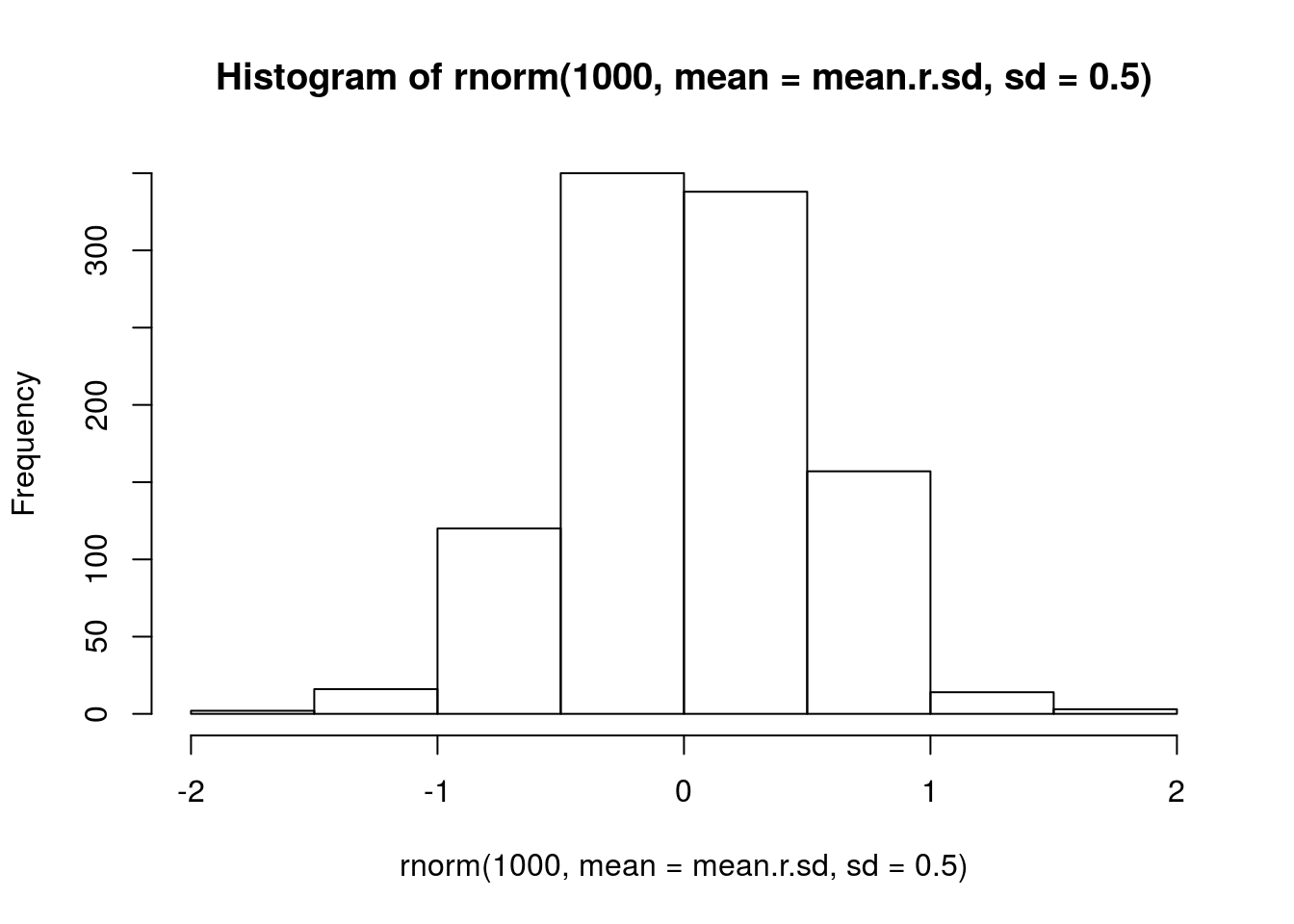
prior.random.effects <- "normal(0.03, 0.5)"

# I don't have a great sense for the growth rate of the parasitoid, other than that it should be negative
# this seems like a reasonable starting point

# visualize prior
hist(rnorm(1000, mean = -1.5, sd = 1))
prior.r.Ptoid <- "normal(-1.5, 1)"Intra- and interspecific interactions
I assume they are weak, i.e. much less than \(|1|\). I also assume that all species exhibit intraspecific competition, aphids have negative interspecific effects with each other, but positive interspecific effects on the parasitoid. I also assume parasitoids have negative interspecific effects on the aphids.
## intraspecific, 0 = no density dependence. this occurs because of offset in model.
# visualize prior
hist(rnorm(1000, mean = -0.1, sd = 0.5))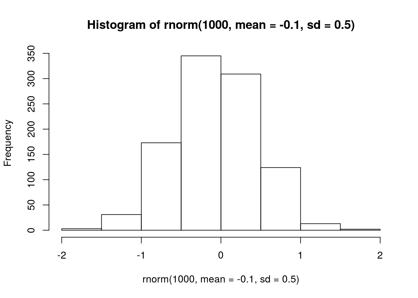
prior.intra.BRBR <- "normal(-0.1, 0.5)"
prior.intra.LYER <- "normal(-0.1, 0.5)"
prior.intra.Ptoid <- "normal(-0.1, 0.5)"

## negative interspecific, 0 = no interaction
# visualize prior
hist(rnorm(1000, mean = -0.1, sd = 0.5))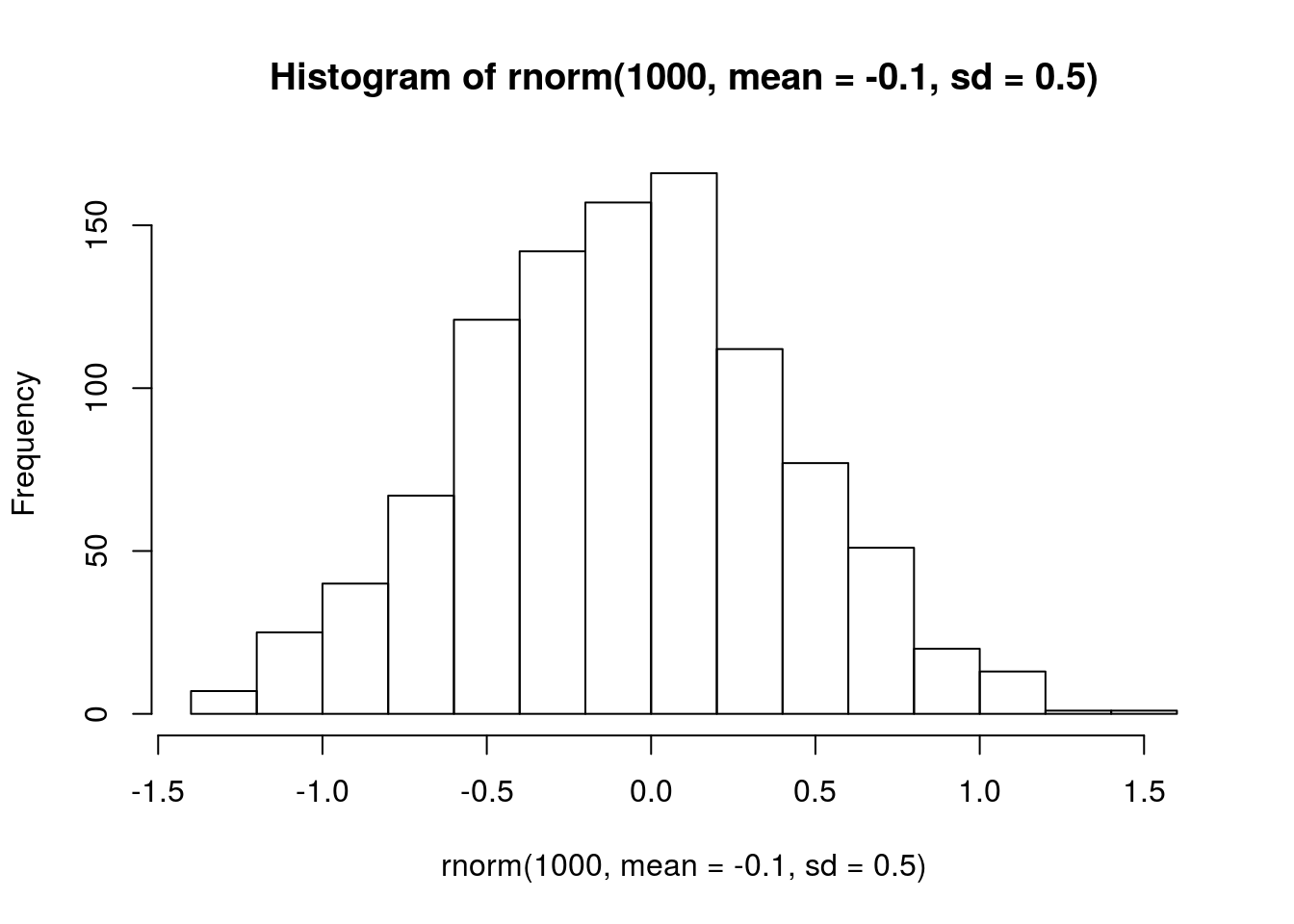
# most of these values are less than 1, which
# is indicative of saturating effects
prior.LYERonBRBR <- "normal(-0.1, 0.5)"
prior.PtoidonBRBR <- "normal(-0.1, 0.5)"
prior.BRBRonLYER <- "normal(-0.1, 0.5)"
prior.PtoidonLYER <- "normal(-0.1, 0.5)"

## positive interspecific
# visualize prior
hist(rnorm(1000, mean = 0.1, sd = 0.5))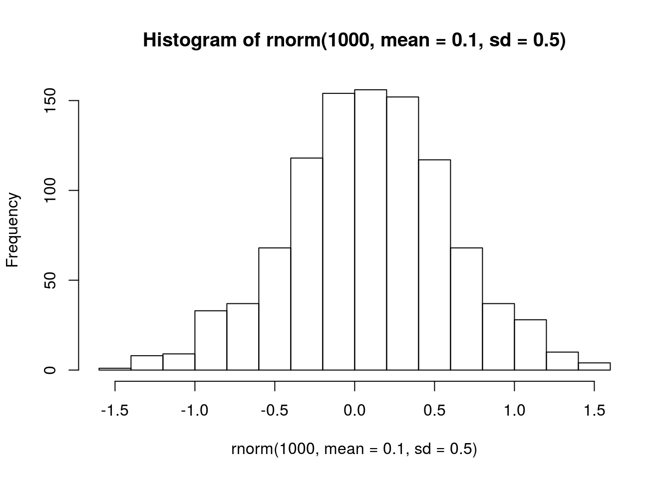
# most of these values are less than 1, which
# is indicative of saturating effects
prior.BRBRonPtoid <- "normal(0.1, 0.5)"
prior.LYERonPtoid <- "normal(0.1, 0.5)"
AOP2 effects
It was unclear to me a priori exactly how allelic differences at AOP2 would affect species’ growth rates or intra- and interspecific interactions. Therefore, I assumed these effects on specific rates could be positive or negative, but would likely be between -1 and 1 (i.e., not ridiculously large).
prior.rich <- "normal(0, 0.5)"Note that in a previous version of this analysis I assessed the effects of genetic diversity, which is why this is called prior.rich. The prior remains the same though, as including both AOP2\(-\) and AOP2\(+\) in the same model corresponds to the effect of genetic diversity (i.e. average effect of adding one genotype to the population).
Temperature effects
As with AOP2 it was unclear to me a priori how warming would affect species’ growth rates or intra- and interspecific interactions; therefore, I used the same prior as for AOP2.
prior.temp <- "normal(0, 0.5)"Biomass effects
For both aphids, I thought that increasing biomass would increase their intrinsic growth rates, but only weakly, because I didn’t expect biomass to be limiting.
# visualize prior
hist(rnorm(1000, mean = 0.1, sd = 0.5))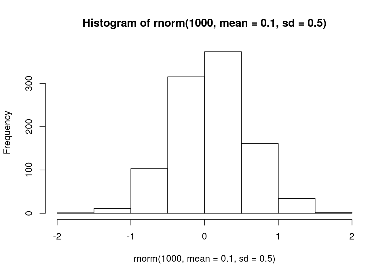
prior.AphidBiomass <- "normal(0.1, 0.5)"For the parasitoid, it was unclear to me whether increasing biomass would have positive or negative effects. I could imagine both, as increasing biomass may increase the search effort of parasitoids, resulting in a negative effect on their growth rate. Alternatively, more biomass may increase the quality of aphids, which could increase the parasitoid’s growth rate. Therefore, I specified a normal prior with mean = 0 and SD = 0.5, so that most of the distribution lied between -1 and 1 (i.e. saturating negative or positive effects).
# visualize prior
hist(rnorm(1000, mean = 0, sd = 0.5))
prior.PtoidBiomass <- "normal(0, 0.5)"Analysis
I first fit a complete model with AOP2\(-\) (aop2_genotypes), AOP2\(+\) (AOP2_genotypes), and temperature (temp) effects.
full.mv.norm.brm <- brm(
  data = full_df,
  formula = mvbf(full.mv.norm.BRBR.bf, full.mv.norm.LYER.bf, full.mv.norm.Ptoid.bf),
  iter = 4000,
  prior = c(# growth rates
            set_prior(prior.r.BRBR, class = "b", coef = "intercept", resp = "log1pBRBRt1"),
            set_prior(prior.r.LYER, class = "b", coef = "intercept", resp = "log1pLYERt1"),
            set_prior(prior.r.Ptoid, class = "b", coef = "intercept", resp = "log1pPtoidt1"),
            # intraspecific effects
            set_prior(prior.intra.BRBR, class = "b", coef = "log1pBRBR_t", resp = "log1pBRBRt1"),
            set_prior(prior.intra.LYER, class = "b", coef = "log1pLYER_t", resp = "log1pLYERt1"),
            set_prior(prior.intra.LYER, class = "b", coef = "log1pPtoid_t", resp = "log1pPtoidt1"),
            # negative interspecific effects
            set_prior(prior.LYERonBRBR, class = "b", coef = "log1pLYER_t", resp = "log1pBRBRt1"),
            set_prior(prior.BRBRonLYER, class = "b", coef = "log1pBRBR_t", resp = "log1pLYERt1"),
            set_prior(prior.PtoidonBRBR, class = "b", coef = "log1pPtoid_t", resp = "log1pBRBRt1"),
            set_prior(prior.PtoidonLYER, class = "b", coef = "log1pPtoid_t", resp = "log1pLYERt1"),
            # positive interspecific effects
            set_prior(prior.BRBRonPtoid, class = "b", coef = "log1pBRBR_t", resp = "log1pPtoidt1"),
            set_prior(prior.LYERonPtoid, class = "b", coef = "log1pLYER_t", resp = "log1pPtoidt1"),
            # aop2 effects
            set_prior(prior.rich, class = "b", coef = "aop2_genotypes", resp = "log1pBRBRt1"),
            set_prior(prior.rich, class = "b", coef = "aop2_genotypes", resp = "log1pLYERt1"),
            set_prior(prior.rich, class = "b", coef = "aop2_genotypes", resp = "log1pPtoidt1"),
            set_prior(prior.rich, class = "b", coef = "log1pBRBR_t:aop2_genotypes", resp = "log1pBRBRt1"),
            set_prior(prior.rich, class = "b", coef = "log1pBRBR_t:aop2_genotypes", resp = "log1pLYERt1"),
            set_prior(prior.rich, class = "b", coef = "log1pBRBR_t:aop2_genotypes", resp = "log1pPtoidt1"),
            set_prior(prior.rich, class = "b", coef = "log1pLYER_t:aop2_genotypes", resp = "log1pBRBRt1"),
            set_prior(prior.rich, class = "b", coef = "log1pLYER_t:aop2_genotypes", resp = "log1pLYERt1"),
            set_prior(prior.rich, class = "b", coef = "log1pLYER_t:aop2_genotypes", resp = "log1pPtoidt1"),
            set_prior(prior.rich, class = "b", coef = "log1pPtoid_t:aop2_genotypes", resp = "log1pBRBRt1"),
            set_prior(prior.rich, class = "b", coef = "log1pPtoid_t:aop2_genotypes", resp = "log1pLYERt1"),
            set_prior(prior.rich, class = "b", coef = "log1pPtoid_t:aop2_genotypes", resp = "log1pPtoidt1"),
            # AOP2 effects
            set_prior(prior.rich, class = "b", coef = "AOP2_genotypes", resp = "log1pBRBRt1"),
            set_prior(prior.rich, class = "b", coef = "AOP2_genotypes", resp = "log1pLYERt1"),
            set_prior(prior.rich, class = "b", coef = "AOP2_genotypes", resp = "log1pPtoidt1"),
            set_prior(prior.rich, class = "b", coef = "log1pBRBR_t:AOP2_genotypes", resp = "log1pBRBRt1"),
            set_prior(prior.rich, class = "b", coef = "log1pBRBR_t:AOP2_genotypes", resp = "log1pLYERt1"),
            set_prior(prior.rich, class = "b", coef = "log1pBRBR_t:AOP2_genotypes", resp = "log1pPtoidt1"),
            set_prior(prior.rich, class = "b", coef = "log1pLYER_t:AOP2_genotypes", resp = "log1pBRBRt1"),
            set_prior(prior.rich, class = "b", coef = "log1pLYER_t:AOP2_genotypes", resp = "log1pLYERt1"),
            set_prior(prior.rich, class = "b", coef = "log1pLYER_t:AOP2_genotypes", resp = "log1pPtoidt1"),
            set_prior(prior.rich, class = "b", coef = "log1pPtoid_t:AOP2_genotypes", resp = "log1pBRBRt1"),
            set_prior(prior.rich, class = "b", coef = "log1pPtoid_t:AOP2_genotypes", resp = "log1pLYERt1"),
            set_prior(prior.rich, class = "b", coef = "log1pPtoid_t:AOP2_genotypes", resp = "log1pPtoidt1"),
            # temp effects
            set_prior(prior.temp, class = "b", coef = "temp", resp = "log1pBRBRt1"),
            set_prior(prior.temp, class = "b", coef = "temp", resp = "log1pLYERt1"),
            set_prior(prior.temp, class = "b", coef = "temp", resp = "log1pPtoidt1"),
            set_prior(prior.temp, class = "b", coef = "log1pBRBR_t:temp", resp = "log1pBRBRt1"),
            set_prior(prior.temp, class = "b", coef = "log1pBRBR_t:temp", resp = "log1pLYERt1"),
            set_prior(prior.temp, class = "b", coef = "log1pBRBR_t:temp", resp = "log1pPtoidt1"),
            set_prior(prior.temp, class = "b", coef = "log1pLYER_t:temp", resp = "log1pBRBRt1"),
            set_prior(prior.temp, class = "b", coef = "log1pLYER_t:temp", resp = "log1pLYERt1"),
            set_prior(prior.temp, class = "b", coef = "log1pLYER_t:temp", resp = "log1pPtoidt1"),
            set_prior(prior.temp, class = "b", coef = "log1pPtoid_t:temp", resp = "log1pBRBRt1"),
            set_prior(prior.temp, class = "b", coef = "log1pPtoid_t:temp", resp = "log1pLYERt1"),
            set_prior(prior.temp, class = "b", coef = "log1pPtoid_t:temp", resp = "log1pPtoidt1"),
            # biomass effects
            set_prior(prior.AphidBiomass, class = "b", coef = "logBiomass_g_t1", resp = "log1pBRBRt1"),
            set_prior(prior.AphidBiomass, class = "b", coef = "logBiomass_g_t1", resp = "log1pLYERt1"),
            set_prior(prior.PtoidBiomass, class = "b", coef = "logBiomass_g_t1", resp = "log1pPtoidt1"),
            # random effects
            set_prior(prior.random.effects, class = "sd", resp = "log1pBRBRt1"),
            set_prior(prior.random.effects, class = "sd", resp = "log1pLYERt1"),
            set_prior(prior.random.effects, class = "sd", resp = "log1pPtoidt1")),
  file = "output/full.mv.norm.brm.keystone.rds")

# print summary
summary(full.mv.norm.brm)
Family: MV(gaussian, gaussian, gaussian)
Links: mu = identity; sigma = identity
mu = identity; sigma = identity
mu = identity; sigma = identity
Formula: log1p(BRBR_t1) ~ 0 + intercept + offset(log1p(BRBR_t)) + (log1p(BRBR_t) + log1p(LYER_t) + log1p(Ptoid_t)) * (temp + aop2_genotypes + AOP2_genotypes) + log(Biomass_g_t1) + (1 | Cage) + ar(time = Week_match.1p, gr = Cage, p = 1, cov = FALSE)
log1p(LYER_t1) ~ 0 + intercept + offset(log1p(LYER_t)) + (log1p(BRBR_t) + log1p(LYER_t) + log1p(Ptoid_t)) * (temp + aop2_genotypes + AOP2_genotypes) + log(Biomass_g_t1) + (1 | Cage) + ar(time = Week_match.1p, gr = Cage, p = 1, cov = FALSE)
log1p(Ptoid_t1) ~ 0 + intercept + offset(log1p(Ptoid_t)) + (log1p(BRBR_t) + log1p(LYER_t) + log1p(Ptoid_t)) * (temp + aop2_genotypes + AOP2_genotypes) + log(Biomass_g_t1) + (1 | Cage) + ar(time = Week_match.1p, gr = Cage, p = 1, cov = FALSE)
Data: full_df (Number of observations: 264)
Samples: 4 chains, each with iter = 4000; warmup = 2000; thin = 1;
total post-warmup samples = 8000
Correlation Structures:
Estimate Est.Error l-95% CI u-95% CI Rhat Bulk_ESS Tail_ESS
ar_log1pBRBRt1[1] -0.47 0.10 -0.65 -0.27 1.00 3459 4671
ar_log1pLYERt1[1] -0.14 0.11 -0.34 0.09 1.00 6057 6167
ar_log1pPtoidt1[1] -0.50 0.08 -0.66 -0.33 1.00 10763 5975
Group-Level Effects:
~Cage (Number of levels: 60)
Estimate Est.Error l-95% CI u-95% CI Rhat Bulk_ESS
sd(log1pBRBRt1_Intercept) 0.31 0.11 0.05 0.51 1.00 919
sd(log1pLYERt1_Intercept) 0.14 0.09 0.01 0.33 1.00 1600
sd(log1pPtoidt1_Intercept) 0.04 0.03 0.00 0.12 1.00 5292
Tail_ESS
sd(log1pBRBRt1_Intercept) 1227
sd(log1pLYERt1_Intercept) 4030
sd(log1pPtoidt1_Intercept) 4483
Population-Level Effects:
Estimate Est.Error l-95% CI u-95% CI
log1pBRBRt1_intercept 1.66 0.70 0.31 3.06
log1pBRBRt1_log1pBRBR_t 0.09 0.16 -0.22 0.40
log1pBRBRt1_log1pLYER_t -0.04 0.17 -0.37 0.30
log1pBRBRt1_log1pPtoid_t -0.98 0.10 -1.17 -0.79
log1pBRBRt1_temp -0.27 0.28 -0.83 0.27
log1pBRBRt1_aop2_genotypes 0.08 0.39 -0.69 0.81
log1pBRBRt1_AOP2_genotypes -0.06 0.39 -0.82 0.71
log1pBRBRt1_logBiomass_g_t1 -0.24 0.24 -0.72 0.23
log1pBRBRt1_log1pBRBR_t:temp -0.08 0.06 -0.19 0.03
log1pBRBRt1_log1pBRBR_t:aop2_genotypes -0.02 0.09 -0.18 0.14
log1pBRBRt1_log1pBRBR_t:AOP2_genotypes -0.07 0.08 -0.23 0.08
log1pBRBRt1_log1pLYER_t:temp -0.00 0.06 -0.12 0.11
log1pBRBRt1_log1pLYER_t:aop2_genotypes -0.04 0.09 -0.21 0.13
log1pBRBRt1_log1pLYER_t:AOP2_genotypes 0.09 0.08 -0.08 0.24
log1pBRBRt1_log1pPtoid_t:temp 0.12 0.04 0.04 0.20
log1pBRBRt1_log1pPtoid_t:aop2_genotypes 0.11 0.06 -0.00 0.23
log1pBRBRt1_log1pPtoid_t:AOP2_genotypes -0.04 0.06 -0.16 0.07
log1pLYERt1_intercept 3.03 0.68 1.70 4.38
log1pLYERt1_log1pBRBR_t 0.46 0.14 0.19 0.73
log1pLYERt1_log1pLYER_t -0.77 0.15 -1.08 -0.47
log1pLYERt1_log1pPtoid_t -0.74 0.09 -0.92 -0.56
log1pLYERt1_temp 0.08 0.26 -0.43 0.59
log1pLYERt1_aop2_genotypes -0.01 0.36 -0.70 0.71
log1pLYERt1_AOP2_genotypes 0.59 0.36 -0.11 1.29
log1pLYERt1_logBiomass_g_t1 -0.05 0.21 -0.46 0.36
log1pLYERt1_log1pBRBR_t:temp -0.03 0.05 -0.12 0.07
log1pLYERt1_log1pBRBR_t:aop2_genotypes -0.10 0.08 -0.25 0.05
log1pLYERt1_log1pBRBR_t:AOP2_genotypes -0.11 0.07 -0.25 0.02
log1pLYERt1_log1pLYER_t:temp 0.01 0.05 -0.09 0.11
log1pLYERt1_log1pLYER_t:aop2_genotypes 0.07 0.08 -0.08 0.22
log1pLYERt1_log1pLYER_t:AOP2_genotypes 0.02 0.07 -0.13 0.17
log1pLYERt1_log1pPtoid_t:temp -0.01 0.04 -0.09 0.06
log1pLYERt1_log1pPtoid_t:aop2_genotypes 0.11 0.06 0.01 0.22
log1pLYERt1_log1pPtoid_t:AOP2_genotypes -0.11 0.05 -0.21 0.00
log1pPtoidt1_intercept -2.11 0.60 -3.30 -0.94
log1pPtoidt1_log1pBRBR_t 0.51 0.10 0.32 0.70
log1pPtoidt1_log1pLYER_t 0.09 0.12 -0.13 0.32
log1pPtoidt1_log1pPtoid_t -0.08 0.07 -0.21 0.06
log1pPtoidt1_temp 0.47 0.23 0.01 0.91
log1pPtoidt1_aop2_genotypes 0.14 0.34 -0.52 0.81
log1pPtoidt1_AOP2_genotypes -0.36 0.34 -1.03 0.33
log1pPtoidt1_logBiomass_g_t1 -0.77 0.17 -1.10 -0.43
log1pPtoidt1_log1pBRBR_t:temp -0.17 0.03 -0.24 -0.10
log1pPtoidt1_log1pBRBR_t:aop2_genotypes -0.06 0.05 -0.16 0.04
log1pPtoidt1_log1pBRBR_t:AOP2_genotypes -0.06 0.05 -0.15 0.03
log1pPtoidt1_log1pLYER_t:temp 0.03 0.04 -0.05 0.11
log1pPtoidt1_log1pLYER_t:aop2_genotypes 0.02 0.06 -0.09 0.14
log1pPtoidt1_log1pLYER_t:AOP2_genotypes 0.12 0.06 0.01 0.23
log1pPtoidt1_log1pPtoid_t:temp 0.03 0.03 -0.03 0.08
log1pPtoidt1_log1pPtoid_t:aop2_genotypes 0.06 0.04 -0.03 0.14
log1pPtoidt1_log1pPtoid_t:AOP2_genotypes -0.04 0.04 -0.12 0.05
Rhat Bulk_ESS Tail_ESS
log1pBRBRt1_intercept 1.00 7944 6027
log1pBRBRt1_log1pBRBR_t 1.00 4474 5458
log1pBRBRt1_log1pLYER_t 1.00 3890 5233
log1pBRBRt1_log1pPtoid_t 1.00 6127 6113
log1pBRBRt1_temp 1.00 7434 6524
log1pBRBRt1_aop2_genotypes 1.00 9159 6370
log1pBRBRt1_AOP2_genotypes 1.00 8608 6290
log1pBRBRt1_logBiomass_g_t1 1.00 9932 6798
log1pBRBRt1_log1pBRBR_t:temp 1.00 5776 5870
log1pBRBRt1_log1pBRBR_t:aop2_genotypes 1.00 5430 5991
log1pBRBRt1_log1pBRBR_t:AOP2_genotypes 1.00 6455 7067
log1pBRBRt1_log1pLYER_t:temp 1.00 5876 5692
log1pBRBRt1_log1pLYER_t:aop2_genotypes 1.00 5185 5743
log1pBRBRt1_log1pLYER_t:AOP2_genotypes 1.00 6058 6330
log1pBRBRt1_log1pPtoid_t:temp 1.00 6966 6843
log1pBRBRt1_log1pPtoid_t:aop2_genotypes 1.00 6468 6098
log1pBRBRt1_log1pPtoid_t:AOP2_genotypes 1.00 7198 6516
log1pLYERt1_intercept 1.00 6965 5990
log1pLYERt1_log1pBRBR_t 1.00 5218 5603
log1pLYERt1_log1pLYER_t 1.00 5166 5926
log1pLYERt1_log1pPtoid_t 1.00 5785 6635
log1pLYERt1_temp 1.00 7154 6150
log1pLYERt1_aop2_genotypes 1.00 8810 5937
log1pLYERt1_AOP2_genotypes 1.00 8612 6413
log1pLYERt1_logBiomass_g_t1 1.00 10326 6103
log1pLYERt1_log1pBRBR_t:temp 1.00 7095 6140
log1pLYERt1_log1pBRBR_t:aop2_genotypes 1.00 5825 5219
log1pLYERt1_log1pBRBR_t:AOP2_genotypes 1.00 6817 6285
log1pLYERt1_log1pLYER_t:temp 1.00 6409 6299
log1pLYERt1_log1pLYER_t:aop2_genotypes 1.00 5583 5710
log1pLYERt1_log1pLYER_t:AOP2_genotypes 1.00 6447 6026
log1pLYERt1_log1pPtoid_t:temp 1.00 8368 6836
log1pLYERt1_log1pPtoid_t:aop2_genotypes 1.00 6783 6242
log1pLYERt1_log1pPtoid_t:AOP2_genotypes 1.00 7780 6627
log1pPtoidt1_intercept 1.00 6000 5841
log1pPtoidt1_log1pBRBR_t 1.00 7508 6234
log1pPtoidt1_log1pLYER_t 1.00 5773 6074
log1pPtoidt1_log1pPtoid_t 1.00 6550 6132
log1pPtoidt1_temp 1.00 6574 5690
log1pPtoidt1_aop2_genotypes 1.00 7574 6101
log1pPtoidt1_AOP2_genotypes 1.00 7131 5984
log1pPtoidt1_logBiomass_g_t1 1.00 11457 6585
log1pPtoidt1_log1pBRBR_t:temp 1.00 8851 6041
log1pPtoidt1_log1pBRBR_t:aop2_genotypes 1.00 8913 5663
log1pPtoidt1_log1pBRBR_t:AOP2_genotypes 1.00 9908 6458
log1pPtoidt1_log1pLYER_t:temp 1.00 7510 5666
log1pPtoidt1_log1pLYER_t:aop2_genotypes 1.00 6799 6398
log1pPtoidt1_log1pLYER_t:AOP2_genotypes 1.00 7319 6417
log1pPtoidt1_log1pPtoid_t:temp 1.00 7660 6157
log1pPtoidt1_log1pPtoid_t:aop2_genotypes 1.00 7282 6258
log1pPtoidt1_log1pPtoid_t:AOP2_genotypes 1.00 8621 6077
Family Specific Parameters:
Estimate Est.Error l-95% CI u-95% CI Rhat Bulk_ESS Tail_ESS
sigma_log1pBRBRt1 1.09 0.06 0.98 1.21 1.00 2301 4483
sigma_log1pLYERt1 0.91 0.04 0.83 0.99 1.00 7388 6274
sigma_log1pPtoidt1 0.76 0.03 0.69 0.83 1.00 13820 5807
Residual Correlations:
Estimate Est.Error l-95% CI u-95% CI Rhat
rescor(log1pBRBRt1,log1pLYERt1) 0.51 0.05 0.40 0.61 1.00
rescor(log1pBRBRt1,log1pPtoidt1) -0.07 0.07 -0.21 0.07 1.00
rescor(log1pLYERt1,log1pPtoidt1) 0.02 0.07 -0.11 0.15 1.00
Bulk_ESS Tail_ESS
rescor(log1pBRBRt1,log1pLYERt1) 6490 6463
rescor(log1pBRBRt1,log1pPtoidt1) 10375 6715
rescor(log1pLYERt1,log1pPtoidt1) 13143 6359
Samples were drawn using sampling(NUTS). For each parameter, Bulk_ESS
and Tail_ESS are effective sample size measures, and Rhat is the potential
scale reduction factor on split chains (at convergence, Rhat = 1).Inspect credible intervals
Below, I inspect which parameters may be safely omitted from the model. It seemed reasonable that if 90% of the posterior probability distribution of the parameter included zero, then I could safely drop it from the model. Therefore, I proceeded with this criteria, starting with the highest-order terms:
# higher-order temperature effects
bayesplot::mcmc_intervals(full.mv.norm.brm, regex_pars = "_t:temp$", prob = 0.66, prob_outer = 0.90) # suggests dropping all, but temp effect on reciprocoal BRBR-Ptoid interaction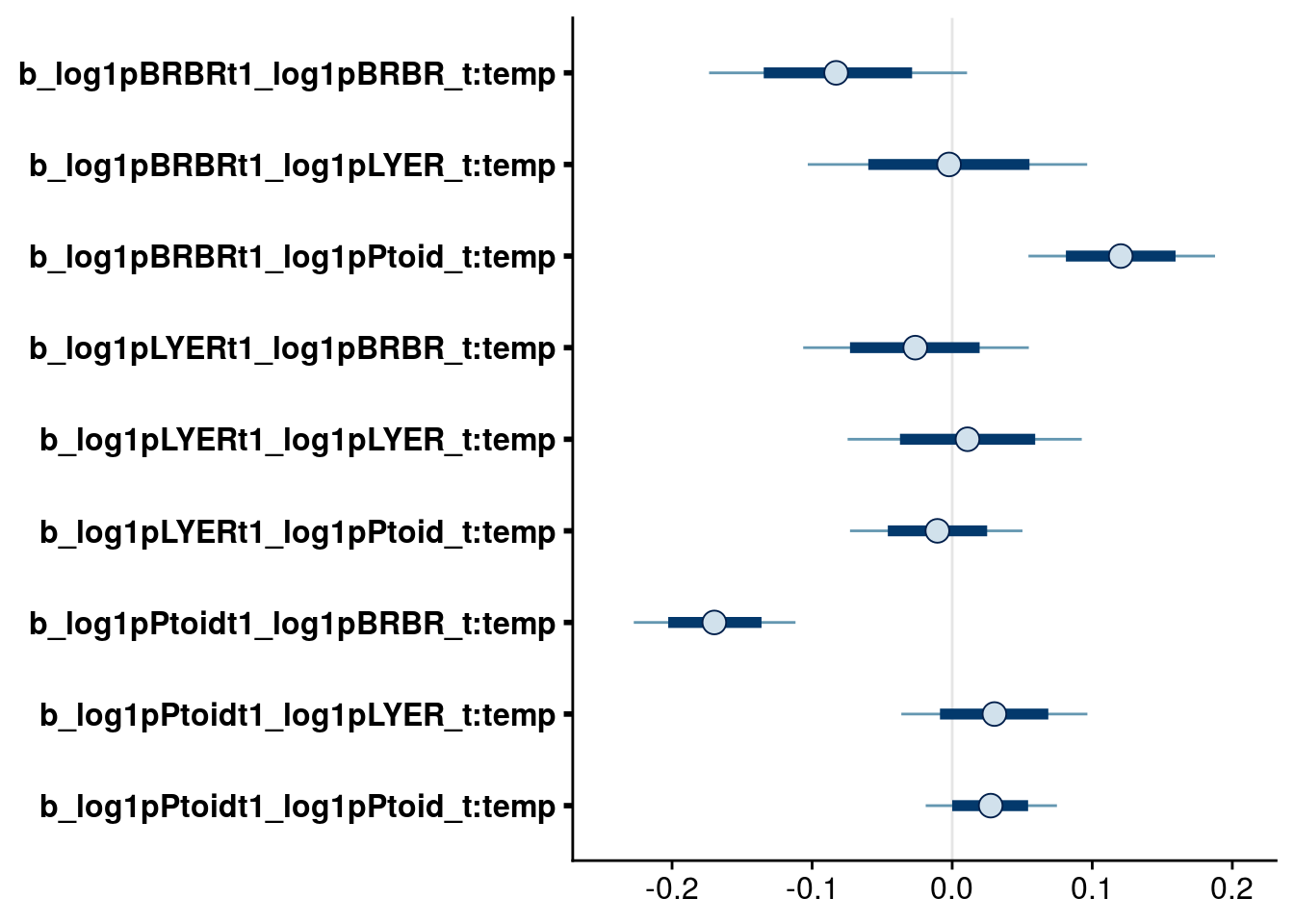
# higher-order aop2 effects
bayesplot::mcmc_intervals(full.mv.norm.brm, regex_pars = "_t:aop2_genotypes$", prob = 0.66, prob_outer = 0.90) # suggests dropping all but AOP2- effects on Ptoid interactions with LYER and BRBR.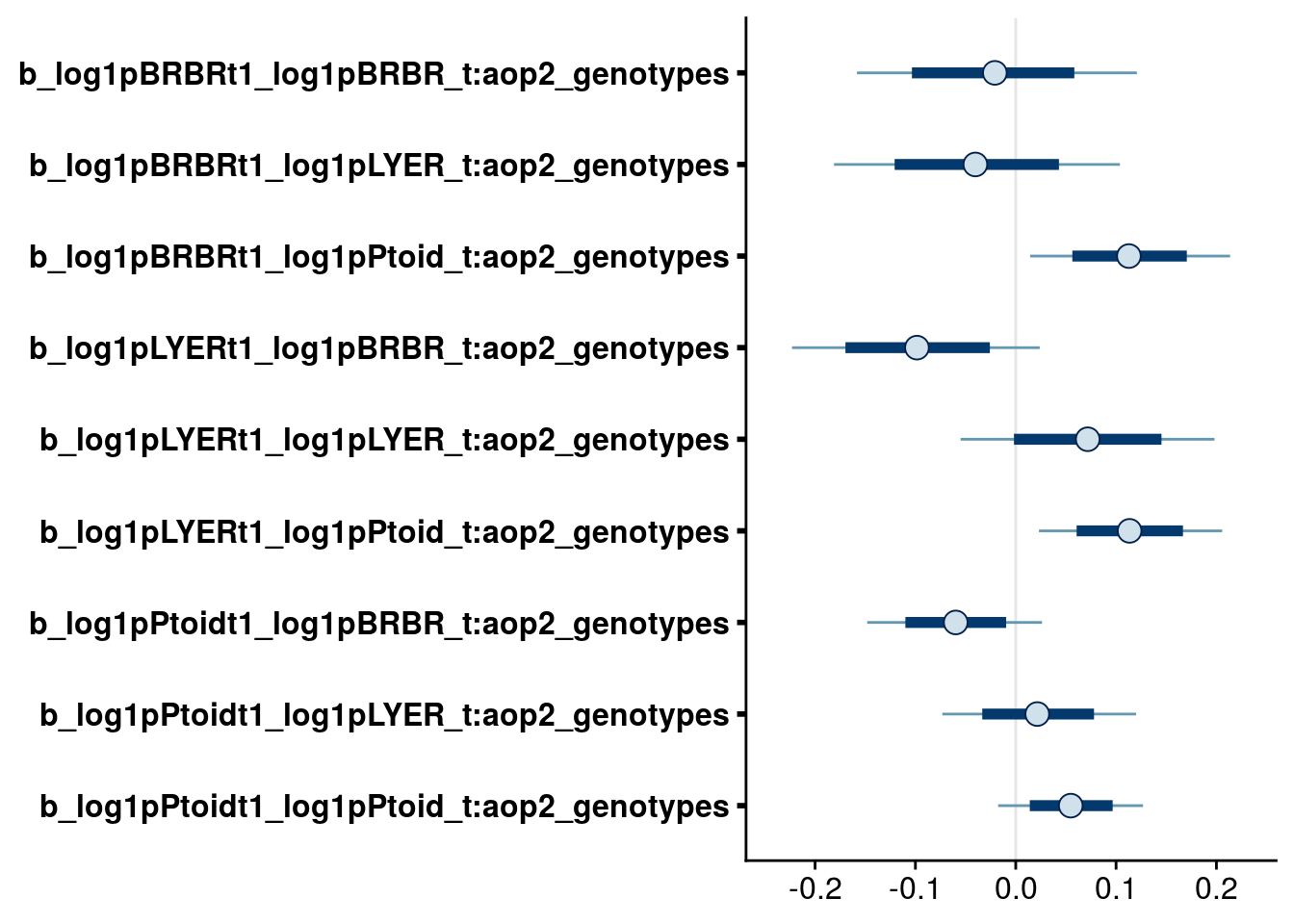
# check biomass effects
bayesplot::mcmc_intervals(full.mv.norm.brm, regex_pars = "_logBiomass_g_t1$", prob = 0.66, prob_outer = 0.90) # drop biomass effect on BRBR and LYER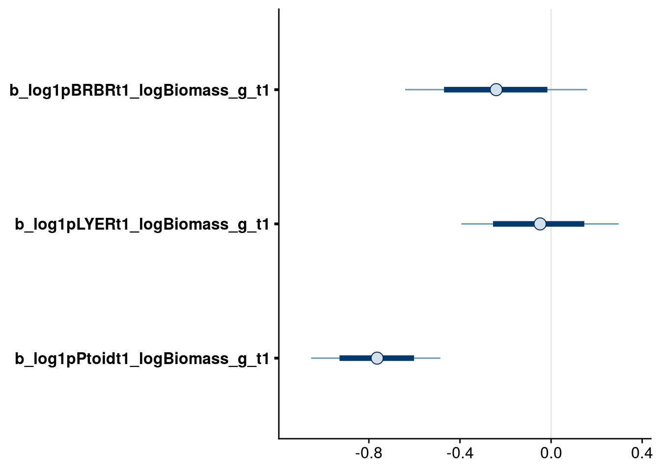
# other terms currently have higher-order effects with temp and AOP2 present,
# need to drop these higher-order terms before examining these main effects
I focus on aop2_genotypes effects, but I make sure to always include AOP2_genotypes in the model. That way, I’m estimating the effect of genotypes with null AOP2\(-\) allele after controlling for the effect of genotypes with a functional AOP2\(+\) allele.
Let’s check how the full model does in reproducing the observed effects of the null AOP2\(-\) in increasing LYER-Ptoid persistence.
pp_aop2_LP_persist(full.mv.norm.brm)aop2_LPbound_BayesP aop2_LPbound_effect
0.326000 -5.957124 aop2_LPbound_BayesP calculates the percentage of posterior samples where the null AOP2\(-\) allele increases LYER-Ptoid persistence relative to the functional AOP2\(+\) allele (as inferred by an increase in its normalized angle). aop2_LPbound_effect calculates the change in the normalized angle from the LYER-Ptoid feasibility boundary for AOP2\(-\) relative to AOP2\(+\). As you can see, the full model is unable to reproduce the observed effects of the null AOP2\(-\) allele in increasing LYER-Ptoid persistence.
Model selection
Reduced model 1
Drop terms
Based on the above plots, I dropped the following higher-order terms:
Effects on BRBR_t1:
(log1p(LYER_t) + log1p(BRBR_t)):temp(log1p(LYER_t) + log1p(BRBR_t)):aop2log(Biomass_g_t1)
Effects on LYER_t1:
(log1p(LYER_t) + log1p(BRBR_t) + log1p(Ptoid_t)):temp(log1p(LYER_t) + log1p(BRBR_t)):aop2log(Biomass_g_t1)
Effects on Ptoid_t1
(log1p(LYER_t) + log1p(Ptoid_t)):temp(log1p(LYER_t) + log1p(BRBR_t) + log1p(Ptoid_t)):aop2
Refit model
# update formulas
reduced.1.BRBR.bf <- update(full.mv.norm.BRBR.bf, .~.
                            -(log1p(LYER_t) + log1p(BRBR_t)):aop2_genotypes
                            -(log1p(LYER_t) + log1p(BRBR_t)):AOP2_genotypes
                            -(log1p(LYER_t) + log1p(BRBR_t)):temp
                            -log(Biomass_g_t1))
reduced.1.LYER.bf <- update(full.mv.norm.LYER.bf, .~.
                            -(log1p(LYER_t) + log1p(BRBR_t) + log1p(Ptoid_t)):temp
                            -(log1p(LYER_t) + log1p(BRBR_t)):aop2_genotypes
                            -(log1p(LYER_t) + log1p(BRBR_t)):AOP2_genotypes
                            -log(Biomass_g_t1))
reduced.1.Ptoid.bf <- update(full.mv.norm.Ptoid.bf, .~.
                             -(log1p(LYER_t) + log1p(Ptoid_t)):temp
                             -(log1p(LYER_t) + log1p(BRBR_t) + log1p(Ptoid_t)):aop2_genotypes
                             -(log1p(LYER_t) + log1p(BRBR_t) + log1p(Ptoid_t)):AOP2_genotypes)

# fit update model
reduced.1.brm <- brm(
  data = full_df,
  formula = mvbf(reduced.1.BRBR.bf, reduced.1.LYER.bf, reduced.1.Ptoid.bf),
  iter = 4000,
  prior = c(# growth rates
            set_prior(prior.r.BRBR, class = "b", coef = "intercept", resp = "log1pBRBRt1"),
            set_prior(prior.r.LYER, class = "b", coef = "intercept", resp = "log1pLYERt1"),
            set_prior(prior.r.Ptoid, class = "b", coef = "intercept", resp = "log1pPtoidt1"),
            # intraspecific effects
            set_prior(prior.intra.BRBR, class = "b", coef = "log1pBRBR_t", resp = "log1pBRBRt1"),
            set_prior(prior.intra.LYER, class = "b", coef = "log1pLYER_t", resp = "log1pLYERt1"),
            set_prior(prior.intra.LYER, class = "b", coef = "log1pPtoid_t", resp = "log1pPtoidt1"),
            # negative interspecific effects
            set_prior(prior.LYERonBRBR, class = "b", coef = "log1pLYER_t", resp = "log1pBRBRt1"),
            set_prior(prior.BRBRonLYER, class = "b", coef = "log1pBRBR_t", resp = "log1pLYERt1"),
            set_prior(prior.PtoidonBRBR, class = "b", coef = "log1pPtoid_t", resp = "log1pBRBRt1"),
            set_prior(prior.PtoidonLYER, class = "b", coef = "log1pPtoid_t", resp = "log1pLYERt1"),
            # positive interspecific effects
            set_prior(prior.BRBRonPtoid, class = "b", coef = "log1pBRBR_t", resp = "log1pPtoidt1"),
            set_prior(prior.LYERonPtoid, class = "b", coef = "log1pLYER_t", resp = "log1pPtoidt1"),
            # aop2 effects
            set_prior(prior.rich, class = "b", coef = "aop2_genotypes", resp = "log1pBRBRt1"),
            set_prior(prior.rich, class = "b", coef = "aop2_genotypes", resp = "log1pLYERt1"),
            set_prior(prior.rich, class = "b", coef = "aop2_genotypes", resp = "log1pPtoidt1"),
            #set_prior(prior.rich, class = "b", coef = "log1pBRBR_t:aop2_genotypes", resp = "log1pBRBRt1"),
            #set_prior(prior.rich, class = "b", coef = "log1pBRBR_t:aop2_genotypes", resp = "log1pLYERt1"),
            #set_prior(prior.rich, class = "b", coef = "log1pBRBR_t:aop2_genotypes", resp = "log1pPtoidt1"),
            #set_prior(prior.rich, class = "b", coef = "log1pLYER_t:aop2_genotypes", resp = "log1pBRBRt1"),
            #set_prior(prior.rich, class = "b", coef = "log1pLYER_t:aop2_genotypes", resp = "log1pLYERt1"),
            #set_prior(prior.rich, class = "b", coef = "log1pLYER_t:aop2_genotypes", resp = "log1pPtoidt1"),
            set_prior(prior.rich, class = "b", coef = "log1pPtoid_t:aop2_genotypes", resp = "log1pBRBRt1"),
            set_prior(prior.rich, class = "b", coef = "log1pPtoid_t:aop2_genotypes", resp = "log1pLYERt1"),
            #set_prior(prior.rich, class = "b", coef = "log1pPtoid_t:aop2_genotypes", resp = "log1pPtoidt1"),
            # AOP2 effects
            set_prior(prior.rich, class = "b", coef = "AOP2_genotypes", resp = "log1pBRBRt1"),
            set_prior(prior.rich, class = "b", coef = "AOP2_genotypes", resp = "log1pLYERt1"),
            set_prior(prior.rich, class = "b", coef = "AOP2_genotypes", resp = "log1pPtoidt1"),
            #set_prior(prior.rich, class = "b", coef = "log1pBRBR_t:AOP2_genotypes", resp = "log1pBRBRt1"),
            #set_prior(prior.rich, class = "b", coef = "log1pBRBR_t:AOP2_genotypes", resp = "log1pLYERt1"),
            #set_prior(prior.rich, class = "b", coef = "log1pBRBR_t:AOP2_genotypes", resp = "log1pPtoidt1"),
            #set_prior(prior.rich, class = "b", coef = "log1pLYER_t:AOP2_genotypes", resp = "log1pBRBRt1"),
            #set_prior(prior.rich, class = "b", coef = "log1pLYER_t:AOP2_genotypes", resp = "log1pLYERt1"),
            #set_prior(prior.rich, class = "b", coef = "log1pLYER_t:AOP2_genotypes", resp = "log1pPtoidt1"),
            set_prior(prior.rich, class = "b", coef = "log1pPtoid_t:AOP2_genotypes", resp = "log1pBRBRt1"),
            set_prior(prior.rich, class = "b", coef = "log1pPtoid_t:AOP2_genotypes", resp = "log1pLYERt1"),
            #set_prior(prior.rich, class = "b", coef = "log1pPtoid_t:AOP2_genotypes", resp = "log1pPtoidt1"),
            # temp effects
            set_prior(prior.temp, class = "b", coef = "temp", resp = "log1pBRBRt1"),
            set_prior(prior.temp, class = "b", coef = "temp", resp = "log1pLYERt1"),
            set_prior(prior.temp, class = "b", coef = "temp", resp = "log1pPtoidt1"),
            #set_prior(prior.temp, class = "b", coef = "log1pBRBR_t:temp", resp = "log1pBRBRt1"),
            #set_prior(prior.temp, class = "b", coef = "log1pBRBR_t:temp", resp = "log1pLYERt1"),
            set_prior(prior.temp, class = "b", coef = "log1pBRBR_t:temp", resp = "log1pPtoidt1"),
            #set_prior(prior.temp, class = "b", coef = "log1pLYER_t:temp", resp = "log1pBRBRt1"),
            #set_prior(prior.temp, class = "b", coef = "log1pLYER_t:temp", resp = "log1pLYERt1"),
            #set_prior(prior.temp, class = "b", coef = "log1pLYER_t:temp", resp = "log1pPtoidt1"),
            set_prior(prior.temp, class = "b", coef = "log1pPtoid_t:temp", resp = "log1pBRBRt1"),
            #set_prior(prior.temp, class = "b", coef = "log1pPtoid_t:temp", resp = "log1pLYERt1"),
            #set_prior(prior.temp, class = "b", coef = "log1pPtoid_t:temp", resp = "log1pPtoidt1"),
            # biomass effects
            #set_prior(prior.AphidBiomass, class = "b", coef = "logBiomass_g_t1", resp = "log1pBRBRt1"),
            #set_prior(prior.AphidBiomass, class = "b", coef = "logBiomass_g_t1", resp = "log1pLYERt1"),
            set_prior(prior.PtoidBiomass, class = "b", coef = "logBiomass_g_t1", resp = "log1pPtoidt1"),
            # random effects
            set_prior(prior.random.effects, class = "sd", resp = "log1pBRBRt1"),
            set_prior(prior.random.effects, class = "sd", resp = "log1pLYERt1"),
            set_prior(prior.random.effects, class = "sd", resp = "log1pPtoidt1")),
  file = "output/reduced.1.brm.keystone.rds")

# print model summary
summary(reduced.1.brm)
Family: MV(gaussian, gaussian, gaussian)
Links: mu = identity; sigma = identity
mu = identity; sigma = identity
mu = identity; sigma = identity
Formula: log1p(BRBR_t1) ~ intercept + log1p(BRBR_t) + log1p(LYER_t) + log1p(Ptoid_t) + temp + aop2_genotypes + AOP2_genotypes + (1 | Cage) + ar(time = Week_match.1p, gr = Cage, p = 1, cov = FALSE) + log1p(Ptoid_t):temp + log1p(Ptoid_t):aop2_genotypes + log1p(Ptoid_t):AOP2_genotypes + offset(log1p(BRBR_t)) - 1
log1p(LYER_t1) ~ intercept + log1p(BRBR_t) + log1p(LYER_t) + log1p(Ptoid_t) + temp + aop2_genotypes + AOP2_genotypes + (1 | Cage) + ar(time = Week_match.1p, gr = Cage, p = 1, cov = FALSE) + log1p(Ptoid_t):aop2_genotypes + log1p(Ptoid_t):AOP2_genotypes + offset(log1p(LYER_t)) - 1
log1p(Ptoid_t1) ~ intercept + log1p(BRBR_t) + log1p(LYER_t) + log1p(Ptoid_t) + temp + aop2_genotypes + AOP2_genotypes + log(Biomass_g_t1) + (1 | Cage) + ar(time = Week_match.1p, gr = Cage, p = 1, cov = FALSE) + log1p(BRBR_t):temp + offset(log1p(Ptoid_t)) - 1
Data: full_df (Number of observations: 264)
Samples: 4 chains, each with iter = 4000; warmup = 2000; thin = 1;
total post-warmup samples = 8000
Correlation Structures:
Estimate Est.Error l-95% CI u-95% CI Rhat Bulk_ESS Tail_ESS
ar_log1pBRBRt1[1] -0.43 0.09 -0.62 -0.24 1.00 3321 4350
ar_log1pLYERt1[1] -0.08 0.10 -0.28 0.14 1.00 5321 5660
ar_log1pPtoidt1[1] -0.47 0.08 -0.63 -0.31 1.00 10081 6281
Group-Level Effects:
~Cage (Number of levels: 60)
Estimate Est.Error l-95% CI u-95% CI Rhat Bulk_ESS
sd(log1pBRBRt1_Intercept) 0.29 0.11 0.04 0.49 1.00 974
sd(log1pLYERt1_Intercept) 0.15 0.09 0.01 0.34 1.00 1461
sd(log1pPtoidt1_Intercept) 0.04 0.03 0.00 0.12 1.00 5171
Tail_ESS
sd(log1pBRBRt1_Intercept) 1090
sd(log1pLYERt1_Intercept) 2928
sd(log1pPtoidt1_Intercept) 4125
Population-Level Effects:
Estimate Est.Error l-95% CI u-95% CI
log1pBRBRt1_intercept 1.86 0.51 0.84 2.85
log1pBRBRt1_log1pBRBR_t -0.07 0.09 -0.25 0.10
log1pBRBRt1_log1pLYER_t 0.06 0.11 -0.15 0.27
log1pBRBRt1_log1pPtoid_t -0.97 0.10 -1.16 -0.78
log1pBRBRt1_temp -0.72 0.09 -0.89 -0.55
log1pBRBRt1_aop2_genotypes -0.24 0.17 -0.57 0.10
log1pBRBRt1_AOP2_genotypes 0.15 0.17 -0.18 0.47
log1pBRBRt1_log1pPtoid_t:temp 0.16 0.03 0.10 0.22
log1pBRBRt1_log1pPtoid_t:aop2_genotypes 0.11 0.06 -0.00 0.23
log1pBRBRt1_log1pPtoid_t:AOP2_genotypes -0.06 0.06 -0.17 0.05
log1pLYERt1_intercept 3.60 0.51 2.62 4.62
log1pLYERt1_log1pBRBR_t 0.22 0.08 0.07 0.38
log1pLYERt1_log1pLYER_t -0.68 0.11 -0.90 -0.48
log1pLYERt1_log1pPtoid_t -0.74 0.09 -0.92 -0.55
log1pLYERt1_temp 0.01 0.06 -0.10 0.12
log1pLYERt1_aop2_genotypes -0.03 0.16 -0.35 0.29
log1pLYERt1_AOP2_genotypes 0.18 0.16 -0.13 0.49
log1pLYERt1_log1pPtoid_t:aop2_genotypes 0.09 0.06 -0.02 0.20
log1pLYERt1_log1pPtoid_t:AOP2_genotypes -0.10 0.05 -0.21 0.00
log1pPtoidt1_intercept -2.62 0.48 -3.58 -1.71
log1pPtoidt1_log1pBRBR_t 0.35 0.06 0.22 0.47
log1pPtoidt1_log1pLYER_t 0.32 0.07 0.18 0.46
log1pPtoidt1_log1pPtoid_t -0.04 0.04 -0.11 0.03
log1pPtoidt1_temp 0.67 0.12 0.44 0.90
log1pPtoidt1_aop2_genotypes 0.12 0.06 -0.00 0.25
log1pPtoidt1_AOP2_genotypes -0.09 0.06 -0.20 0.02
log1pPtoidt1_logBiomass_g_t1 -0.76 0.17 -1.09 -0.41
log1pPtoidt1_log1pBRBR_t:temp -0.17 0.02 -0.22 -0.12
Rhat Bulk_ESS Tail_ESS
log1pBRBRt1_intercept 1.00 6157 5398
log1pBRBRt1_log1pBRBR_t 1.00 3181 4898
log1pBRBRt1_log1pLYER_t 1.00 2789 4943
log1pBRBRt1_log1pPtoid_t 1.00 4025 5440
log1pBRBRt1_temp 1.00 5759 5772
log1pBRBRt1_aop2_genotypes 1.00 4990 5437
log1pBRBRt1_AOP2_genotypes 1.00 5360 5945
log1pBRBRt1_log1pPtoid_t:temp 1.00 7507 5961
log1pBRBRt1_log1pPtoid_t:aop2_genotypes 1.00 4454 5503
log1pBRBRt1_log1pPtoid_t:AOP2_genotypes 1.00 4983 5830
log1pLYERt1_intercept 1.00 5051 5913
log1pLYERt1_log1pBRBR_t 1.00 3986 4881
log1pLYERt1_log1pLYER_t 1.00 3717 4238
log1pLYERt1_log1pPtoid_t 1.00 3874 5325
log1pLYERt1_temp 1.00 4901 5656
log1pLYERt1_aop2_genotypes 1.00 5083 5643
log1pLYERt1_AOP2_genotypes 1.00 4481 5077
log1pLYERt1_log1pPtoid_t:aop2_genotypes 1.00 4544 5624
log1pLYERt1_log1pPtoid_t:AOP2_genotypes 1.00 4541 5230
log1pPtoidt1_intercept 1.00 4473 5102
log1pPtoidt1_log1pBRBR_t 1.00 5813 5444
log1pPtoidt1_log1pLYER_t 1.00 6228 6316
log1pPtoidt1_log1pPtoid_t 1.00 7439 6040
log1pPtoidt1_temp 1.00 5247 5460
log1pPtoidt1_aop2_genotypes 1.00 7483 6501
log1pPtoidt1_AOP2_genotypes 1.00 9384 5787
log1pPtoidt1_logBiomass_g_t1 1.00 5708 5754
log1pPtoidt1_log1pBRBR_t:temp 1.00 5825 6122
Family Specific Parameters:
Estimate Est.Error l-95% CI u-95% CI Rhat Bulk_ESS Tail_ESS
sigma_log1pBRBRt1 1.11 0.06 1.00 1.23 1.00 2840 4430
sigma_log1pLYERt1 0.91 0.04 0.83 1.00 1.00 6503 6666
sigma_log1pPtoidt1 0.76 0.03 0.70 0.84 1.00 14431 5870
Residual Correlations:
Estimate Est.Error l-95% CI u-95% CI Rhat
rescor(log1pBRBRt1,log1pLYERt1) 0.53 0.05 0.43 0.62 1.00
rescor(log1pBRBRt1,log1pPtoidt1) -0.06 0.07 -0.20 0.08 1.00
rescor(log1pLYERt1,log1pPtoidt1) 0.03 0.07 -0.10 0.16 1.00
Bulk_ESS Tail_ESS
rescor(log1pBRBRt1,log1pLYERt1) 7014 6336
rescor(log1pBRBRt1,log1pPtoidt1) 7955 6672
rescor(log1pLYERt1,log1pPtoidt1) 10786 5868
Samples were drawn using sampling(NUTS). For each parameter, Bulk_ESS
and Tail_ESS are effective sample size measures, and Rhat is the potential
scale reduction factor on split chains (at convergence, Rhat = 1).Inspect credible intervals
# higher-order temperature effects
bayesplot::mcmc_intervals(reduced.1.brm, regex_pars = "_t:temp$", prob = 0.66, prob_outer = 0.90) # retain these higher-order effects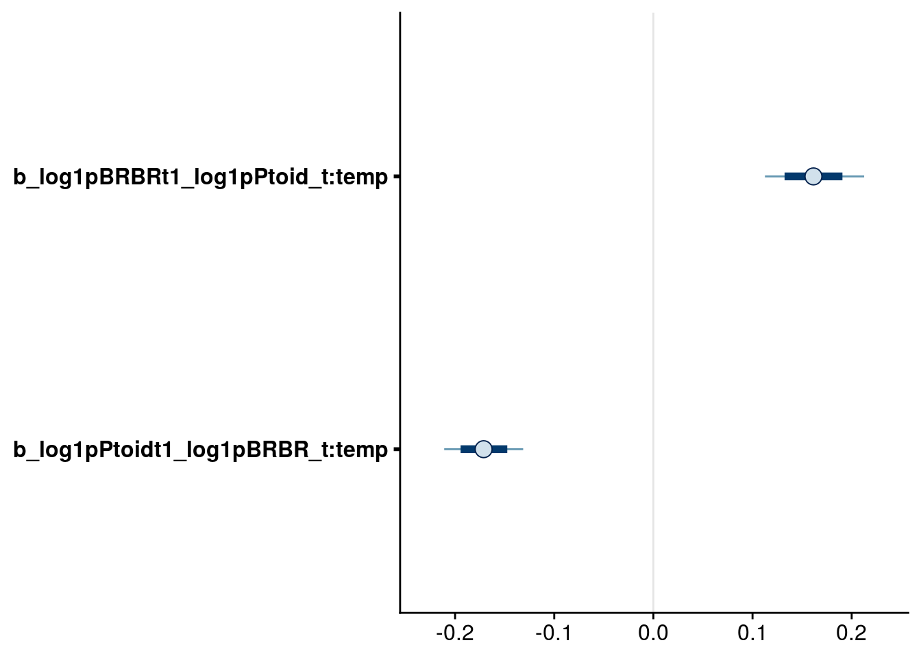
# higher-order aop2 effects
bayesplot::mcmc_intervals(reduced.1.brm, regex_pars = "_t:aop2_genotypes$", prob = 0.66, prob_outer = 0.90) 
# lower-order temp effects
bayesplot::mcmc_intervals(reduced.1.brm, regex_pars = "_temp$", prob = 0.66, prob_outer = 0.90) # drop temp on LYER as there are no higher-order terms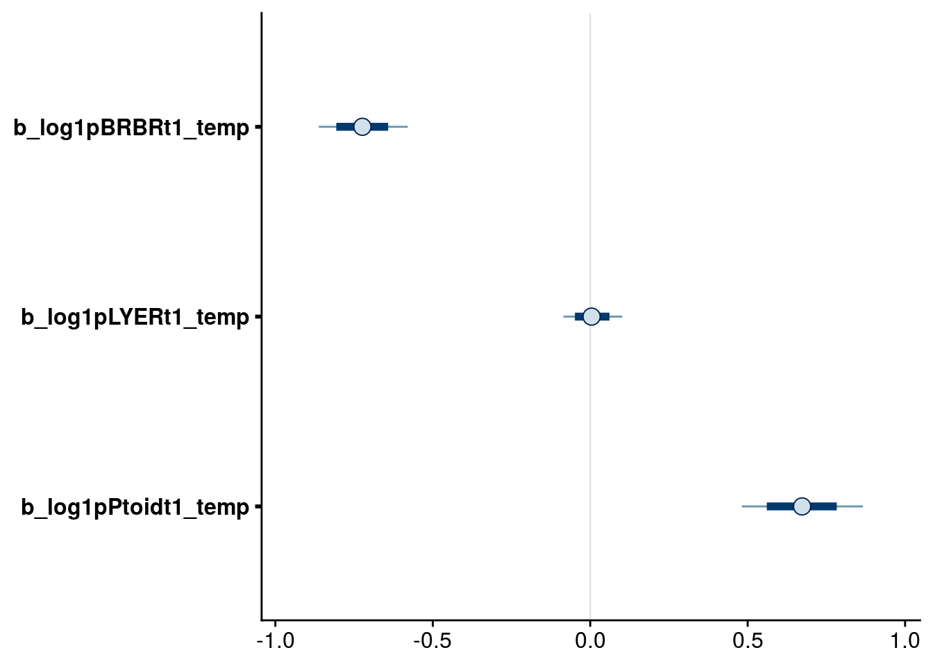
bayesplot::mcmc_intervals(reduced.1.brm, regex_pars = "_aop2_genotypes$", prob = 0.66, prob_outer = 0.90) # retain all, because of higher-order terms for BRBR and LYER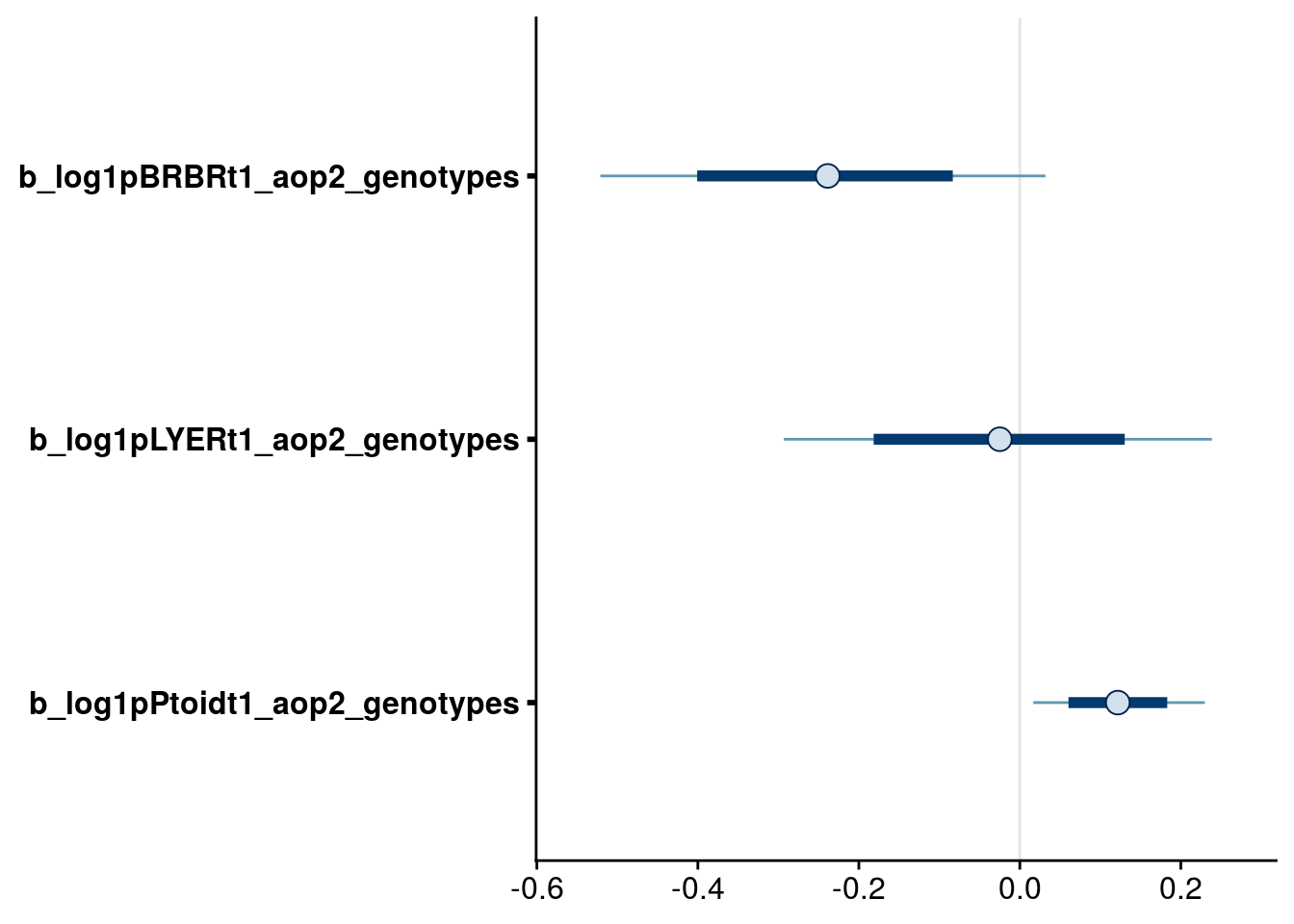
# check biomass effects
bayesplot::mcmc_intervals(reduced.1.brm, regex_pars = "_logBiomass_g_t1$", prob = 0.66, prob_outer = 0.90)
# check other interaction terms
bayesplot::mcmc_intervals(reduced.1.brm, regex_pars = "_log1pPtoid_t$", prob = 0.80, prob_outer = 0.90) # drop intraspecific effect of Ptoid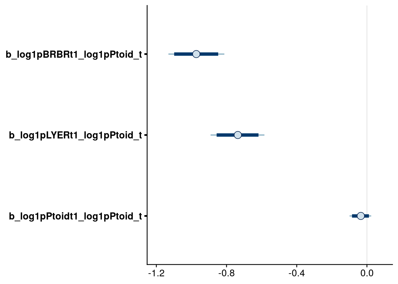
bayesplot::mcmc_intervals(reduced.1.brm, regex_pars = "_log1pLYER_t$", prob = 0.80, prob_outer = 0.90) # drop LYER effect on BRBR
bayesplot::mcmc_intervals(reduced.1.brm, regex_pars = "_log1pBRBR_t$", prob = 0.80, prob_outer = 0.90) # drop intraspecific effect of BRBR
Since there are still terms to drop based on my 90% criteria, Reduced model 1 is an intermediate model that I don’t use in my model comparison.
Reduced model 2
Drop terms
Based on the above plots, I dropped the following terms:
Effects on BRBR_t1:
log1p(BRBR_t)log1p(LYER_t)
Effects on LYER_t1:
temp
Effects on Ptoid_t1:
log1p(Ptoid_t)
Refit model
# update formulas
reduced.2.BRBR.bf <- update(reduced.1.BRBR.bf, .~. -log1p(BRBR_t) -log1p(LYER_t))
reduced.2.LYER.bf <- update(reduced.1.LYER.bf, .~. -temp)
reduced.2.Ptoid.bf <- update(reduced.1.Ptoid.bf, .~. -log1p(Ptoid_t))

# fit new model
reduced.2.brm <- brm(
  data = full_df,
  formula = mvbf(reduced.2.BRBR.bf, reduced.2.LYER.bf, reduced.2.Ptoid.bf),
  iter = 4000,
  prior = c(# growth rates
            set_prior(prior.r.BRBR, class = "b", coef = "intercept", resp = "log1pBRBRt1"),
            set_prior(prior.r.LYER, class = "b", coef = "intercept", resp = "log1pLYERt1"),
            set_prior(prior.r.Ptoid, class = "b", coef = "intercept", resp = "log1pPtoidt1"),
            # intraspecific effects
            #set_prior(prior.intra.BRBR, class = "b", coef = "log1pBRBR_t", resp = "log1pBRBRt1"),
            set_prior(prior.intra.LYER, class = "b", coef = "log1pLYER_t", resp = "log1pLYERt1"),
            #set_prior(prior.intra.LYER, class = "b", coef = "log1pPtoid_t", resp = "log1pPtoidt1"),
            # negative interspecific effects
            #set_prior(prior.LYERonBRBR, class = "b", coef = "log1pLYER_t", resp = "log1pBRBRt1"),
            set_prior(prior.BRBRonLYER, class = "b", coef = "log1pBRBR_t", resp = "log1pLYERt1"),
            set_prior(prior.PtoidonBRBR, class = "b", coef = "log1pPtoid_t", resp = "log1pBRBRt1"),
            set_prior(prior.PtoidonLYER, class = "b", coef = "log1pPtoid_t", resp = "log1pLYERt1"),
            # positive interspecific effects
            set_prior(prior.BRBRonPtoid, class = "b", coef = "log1pBRBR_t", resp = "log1pPtoidt1"),
            set_prior(prior.LYERonPtoid, class = "b", coef = "log1pLYER_t", resp = "log1pPtoidt1"),
            # aop2 effects
            set_prior(prior.rich, class = "b", coef = "aop2_genotypes", resp = "log1pBRBRt1"),
            set_prior(prior.rich, class = "b", coef = "aop2_genotypes", resp = "log1pLYERt1"),
            set_prior(prior.rich, class = "b", coef = "aop2_genotypes", resp = "log1pPtoidt1"),
            #set_prior(prior.rich, class = "b", coef = "log1pBRBR_t:aop2_genotypes", resp = "log1pBRBRt1"),
            #set_prior(prior.rich, class = "b", coef = "log1pBRBR_t:aop2_genotypes", resp = "log1pLYERt1"),
            #set_prior(prior.rich, class = "b", coef = "log1pBRBR_t:aop2_genotypes", resp = "log1pPtoidt1"),
            #set_prior(prior.rich, class = "b", coef = "log1pLYER_t:aop2_genotypes", resp = "log1pBRBRt1"),
            #set_prior(prior.rich, class = "b", coef = "log1pLYER_t:aop2_genotypes", resp = "log1pLYERt1"),
            #set_prior(prior.rich, class = "b", coef = "log1pLYER_t:aop2_genotypes", resp = "log1pPtoidt1"),
            set_prior(prior.rich, class = "b", coef = "log1pPtoid_t:aop2_genotypes", resp = "log1pBRBRt1"),
            set_prior(prior.rich, class = "b", coef = "log1pPtoid_t:aop2_genotypes", resp = "log1pLYERt1"),
            #set_prior(prior.rich, class = "b", coef = "log1pPtoid_t:aop2_genotypes", resp = "log1pPtoidt1"),
            # AOP2 effects
            set_prior(prior.rich, class = "b", coef = "AOP2_genotypes", resp = "log1pBRBRt1"),
            set_prior(prior.rich, class = "b", coef = "AOP2_genotypes", resp = "log1pLYERt1"),
            set_prior(prior.rich, class = "b", coef = "AOP2_genotypes", resp = "log1pPtoidt1"),
            #set_prior(prior.rich, class = "b", coef = "log1pBRBR_t:AOP2_genotypes", resp = "log1pBRBRt1"),
            #set_prior(prior.rich, class = "b", coef = "log1pBRBR_t:AOP2_genotypes", resp = "log1pLYERt1"),
            #set_prior(prior.rich, class = "b", coef = "log1pBRBR_t:AOP2_genotypes", resp = "log1pPtoidt1"),
            #set_prior(prior.rich, class = "b", coef = "log1pLYER_t:AOP2_genotypes", resp = "log1pBRBRt1"),
            #set_prior(prior.rich, class = "b", coef = "log1pLYER_t:AOP2_genotypes", resp = "log1pLYERt1"),
            #set_prior(prior.rich, class = "b", coef = "log1pLYER_t:AOP2_genotypes", resp = "log1pPtoidt1"),
            set_prior(prior.rich, class = "b", coef = "log1pPtoid_t:AOP2_genotypes", resp = "log1pBRBRt1"),
            set_prior(prior.rich, class = "b", coef = "log1pPtoid_t:AOP2_genotypes", resp = "log1pLYERt1"),
            #set_prior(prior.rich, class = "b", coef = "log1pPtoid_t:AOP2_genotypes", resp = "log1pPtoidt1"),
            # temp effects
            set_prior(prior.temp, class = "b", coef = "temp", resp = "log1pBRBRt1"),
            #set_prior(prior.temp, class = "b", coef = "temp", resp = "log1pLYERt1"),
            set_prior(prior.temp, class = "b", coef = "temp", resp = "log1pPtoidt1"),
            #set_prior(prior.temp, class = "b", coef = "log1pBRBR_t:temp", resp = "log1pBRBRt1"),
            #set_prior(prior.temp, class = "b", coef = "log1pBRBR_t:temp", resp = "log1pLYERt1"),
            set_prior(prior.temp, class = "b", coef = "log1pBRBR_t:temp", resp = "log1pPtoidt1"),
            #set_prior(prior.temp, class = "b", coef = "log1pLYER_t:temp", resp = "log1pBRBRt1"),
            #set_prior(prior.temp, class = "b", coef = "log1pLYER_t:temp", resp = "log1pLYERt1"),
            #set_prior(prior.temp, class = "b", coef = "log1pLYER_t:temp", resp = "log1pPtoidt1"),
            set_prior(prior.temp, class = "b", coef = "log1pPtoid_t:temp", resp = "log1pBRBRt1"),
            #set_prior(prior.temp, class = "b", coef = "log1pPtoid_t:temp", resp = "log1pLYERt1"),
            #set_prior(prior.temp, class = "b", coef = "log1pPtoid_t:temp", resp = "log1pPtoidt1"),
            # biomass effects
            #set_prior(prior.AphidBiomass, class = "b", coef = "logBiomass_g_t1", resp = "log1pBRBRt1"),
            #set_prior(prior.AphidBiomass, class = "b", coef = "logBiomass_g_t1", resp = "log1pLYERt1"),
            set_prior(prior.PtoidBiomass, class = "b", coef = "logBiomass_g_t1", resp = "log1pPtoidt1"),
            # random effects
            set_prior(prior.random.effects, class = "sd", resp = "log1pBRBRt1"),
            set_prior(prior.random.effects, class = "sd", resp = "log1pLYERt1"),
            set_prior(prior.random.effects, class = "sd", resp = "log1pPtoidt1")),
  file = "output/reduced.2.brm.keystone.rds")

# print model summary
summary(reduced.2.brm)
Family: MV(gaussian, gaussian, gaussian)
Links: mu = identity; sigma = identity
mu = identity; sigma = identity
mu = identity; sigma = identity
Formula: log1p(BRBR_t1) ~ intercept + log1p(Ptoid_t) + temp + aop2_genotypes + AOP2_genotypes + (1 | Cage) + ar(time = Week_match.1p, gr = Cage, p = 1, cov = FALSE) + log1p(Ptoid_t):temp + log1p(Ptoid_t):aop2_genotypes + log1p(Ptoid_t):AOP2_genotypes + offset(log1p(BRBR_t)) - 1
log1p(LYER_t1) ~ intercept + log1p(BRBR_t) + log1p(LYER_t) + log1p(Ptoid_t) + aop2_genotypes + AOP2_genotypes + (1 | Cage) + ar(time = Week_match.1p, gr = Cage, p = 1, cov = FALSE) + log1p(Ptoid_t):aop2_genotypes + log1p(Ptoid_t):AOP2_genotypes + offset(log1p(LYER_t)) - 1
log1p(Ptoid_t1) ~ intercept + log1p(BRBR_t) + log1p(LYER_t) + temp + aop2_genotypes + AOP2_genotypes + log(Biomass_g_t1) + (1 | Cage) + ar(time = Week_match.1p, gr = Cage, p = 1, cov = FALSE) + log1p(BRBR_t):temp + offset(log1p(Ptoid_t)) - 1
Data: full_df (Number of observations: 264)
Samples: 4 chains, each with iter = 4000; warmup = 2000; thin = 1;
total post-warmup samples = 8000
Correlation Structures:
Estimate Est.Error l-95% CI u-95% CI Rhat Bulk_ESS Tail_ESS
ar_log1pBRBRt1[1] -0.45 0.09 -0.62 -0.27 1.00 4131 5750
ar_log1pLYERt1[1] -0.10 0.09 -0.28 0.09 1.00 6407 6523
ar_log1pPtoidt1[1] -0.49 0.08 -0.65 -0.33 1.00 12076 6190
Group-Level Effects:
~Cage (Number of levels: 60)
Estimate Est.Error l-95% CI u-95% CI Rhat Bulk_ESS
sd(log1pBRBRt1_Intercept) 0.25 0.10 0.03 0.43 1.00 1110
sd(log1pLYERt1_Intercept) 0.14 0.09 0.01 0.32 1.00 1877
sd(log1pPtoidt1_Intercept) 0.04 0.03 0.00 0.11 1.00 4674
Tail_ESS
sd(log1pBRBRt1_Intercept) 1675
sd(log1pLYERt1_Intercept) 3273
sd(log1pPtoidt1_Intercept) 3649
Population-Level Effects:
Estimate Est.Error l-95% CI u-95% CI
log1pBRBRt1_intercept 1.78 0.28 1.22 2.35
log1pBRBRt1_log1pPtoid_t -0.97 0.10 -1.16 -0.79
log1pBRBRt1_temp -0.71 0.08 -0.86 -0.56
log1pBRBRt1_aop2_genotypes -0.25 0.17 -0.58 0.08
log1pBRBRt1_AOP2_genotypes 0.15 0.16 -0.16 0.47
log1pBRBRt1_log1pPtoid_t:temp 0.17 0.03 0.11 0.23
log1pBRBRt1_log1pPtoid_t:aop2_genotypes 0.12 0.06 0.00 0.24
log1pBRBRt1_log1pPtoid_t:AOP2_genotypes -0.06 0.06 -0.17 0.05
log1pLYERt1_intercept 3.51 0.47 2.58 4.44
log1pLYERt1_log1pBRBR_t 0.23 0.05 0.13 0.34
log1pLYERt1_log1pLYER_t -0.67 0.08 -0.83 -0.52
log1pLYERt1_log1pPtoid_t -0.73 0.09 -0.91 -0.55
log1pLYERt1_aop2_genotypes -0.03 0.16 -0.33 0.30
log1pLYERt1_AOP2_genotypes 0.18 0.15 -0.12 0.47
log1pLYERt1_log1pPtoid_t:aop2_genotypes 0.09 0.06 -0.02 0.20
log1pLYERt1_log1pPtoid_t:AOP2_genotypes -0.10 0.05 -0.20 0.00
log1pPtoidt1_intercept -2.89 0.38 -3.66 -2.14
log1pPtoidt1_log1pBRBR_t 0.35 0.06 0.23 0.48
log1pPtoidt1_log1pLYER_t 0.35 0.06 0.23 0.48
log1pPtoidt1_temp 0.67 0.12 0.44 0.90
log1pPtoidt1_aop2_genotypes 0.11 0.06 -0.02 0.24
log1pPtoidt1_AOP2_genotypes -0.08 0.06 -0.19 0.03
log1pPtoidt1_logBiomass_g_t1 -0.73 0.17 -1.06 -0.39
log1pPtoidt1_log1pBRBR_t:temp -0.17 0.02 -0.22 -0.12
Rhat Bulk_ESS Tail_ESS
log1pBRBRt1_intercept 1.00 4258 5480
log1pBRBRt1_log1pPtoid_t 1.00 4185 4922
log1pBRBRt1_temp 1.00 8284 5845
log1pBRBRt1_aop2_genotypes 1.00 5290 5928
log1pBRBRt1_AOP2_genotypes 1.00 5543 6129
log1pBRBRt1_log1pPtoid_t:temp 1.00 8537 5921
log1pBRBRt1_log1pPtoid_t:aop2_genotypes 1.00 5093 5764
log1pBRBRt1_log1pPtoid_t:AOP2_genotypes 1.00 5576 6064
log1pLYERt1_intercept 1.00 5752 6253
log1pLYERt1_log1pBRBR_t 1.00 7208 5388
log1pLYERt1_log1pLYER_t 1.00 5839 5821
log1pLYERt1_log1pPtoid_t 1.00 4785 5511
log1pLYERt1_aop2_genotypes 1.00 6140 5964
log1pLYERt1_AOP2_genotypes 1.00 5914 5975
log1pLYERt1_log1pPtoid_t:aop2_genotypes 1.00 6028 5872
log1pLYERt1_log1pPtoid_t:AOP2_genotypes 1.00 5963 6009
log1pPtoidt1_intercept 1.00 5615 5914
log1pPtoidt1_log1pBRBR_t 1.00 6287 5661
log1pPtoidt1_log1pLYER_t 1.00 7928 6576
log1pPtoidt1_temp 1.00 5426 5126
log1pPtoidt1_aop2_genotypes 1.00 8165 6011
log1pPtoidt1_AOP2_genotypes 1.00 9176 6614
log1pPtoidt1_logBiomass_g_t1 1.00 6590 6103
log1pPtoidt1_log1pBRBR_t:temp 1.00 5636 5247
Family Specific Parameters:
Estimate Est.Error l-95% CI u-95% CI Rhat Bulk_ESS Tail_ESS
sigma_log1pBRBRt1 1.11 0.06 1.00 1.23 1.00 3535 5493
sigma_log1pLYERt1 0.91 0.04 0.83 1.00 1.00 7690 6459
sigma_log1pPtoidt1 0.76 0.03 0.70 0.83 1.00 13065 5490
Residual Correlations:
Estimate Est.Error l-95% CI u-95% CI Rhat
rescor(log1pBRBRt1,log1pLYERt1) 0.52 0.05 0.41 0.61 1.00
rescor(log1pBRBRt1,log1pPtoidt1) -0.05 0.07 -0.19 0.09 1.00
rescor(log1pLYERt1,log1pPtoidt1) 0.03 0.07 -0.10 0.16 1.00
Bulk_ESS Tail_ESS
rescor(log1pBRBRt1,log1pLYERt1) 9083 6456
rescor(log1pBRBRt1,log1pPtoidt1) 10207 6645
rescor(log1pLYERt1,log1pPtoidt1) 13091 6708
Samples were drawn using sampling(NUTS). For each parameter, Bulk_ESS
and Tail_ESS are effective sample size measures, and Rhat is the potential
scale reduction factor on split chains (at convergence, Rhat = 1).Inspect credible intervals
# higher-order aop2 effects
bayesplot::mcmc_intervals(reduced.2.brm, regex_pars = "_t:aop2_genotypes$", prob = 0.66, prob_outer = 0.90) 
# note that one of these intervals doesn't quite meet our 90% criteria and is right on the edge.
broom.mixed::tidy(reduced.2.brm, parameters = "b_log1pLYERt1_log1pPtoid_t:aop2_genotypes", conf.level = 0.90)
# A tibble: 1 x 6
component term estimate std.error conf.low conf.high
<chr> <chr> <dbl> <dbl> <dbl> <dbl>
1 cond b_log1pLYERt1_log1pPtoid_t:ao… 0.0921 0.0565 -5.93e-4 0.183# but since the 90% interval is admittedly a bit arbitrary, we can explore effect effect of retaining all terms in this model.
bayesplot::mcmc_intervals(reduced.2.brm, regex_pars = "_aop2_genotypes$", prob = 0.66, prob_outer = 0.90) # retain all because of presence of higher-order terms
Now let’s check how well the model performed in capturing the effect of AOP2\(-\) on LYER-Ptoid persistence.
pp_aop2_LP_persist(reduced.2.brm, temp.cond = 1.5, aop2.cond = 2)aop2_LPbound_BayesP aop2_LPbound_effect
0.727250 2.300524 Only 73% of the posterior samples support a positive effect of AOP2\(-\) relative to AOP2\(+\) on LYER-Ptoid persistence. Note that we are still on our way to identify a model based on the 90% cutoff, but I show it above to show that this model still doesn’t appear to adequately capture the effect of AOP2.
Reduced model 3
Drop terms
Based on the above plots, we will drop the following term:
Effects on BRBR_t1:
- keep all
Effects on LYER_t1:
log1p(Ptoid_t):aop2_genotypes
Effects on Ptoid_t1:
- keep all
Refit model
# update formulas
reduced.3.BRBR.bf <- reduced.2.BRBR.bf
reduced.3.LYER.bf <- update(reduced.2.LYER.bf, .~. -log1p(Ptoid_t):aop2_genotypes -log1p(Ptoid_t):AOP2_genotypes)
reduced.3.Ptoid.bf <- reduced.2.Ptoid.bf

# fit new model
reduced.3.brm <- brm(
  data = full_df,
  formula = mvbf(reduced.3.BRBR.bf, reduced.3.LYER.bf, reduced.3.Ptoid.bf),
  iter = 4000,
  prior = c(# growth rates
            set_prior(prior.r.BRBR, class = "b", coef = "intercept", resp = "log1pBRBRt1"),
            set_prior(prior.r.LYER, class = "b", coef = "intercept", resp = "log1pLYERt1"),
            set_prior(prior.r.Ptoid, class = "b", coef = "intercept", resp = "log1pPtoidt1"),
            # intraspecific effects
            #set_prior(prior.intra.BRBR, class = "b", coef = "log1pBRBR_t", resp = "log1pBRBRt1"),
            set_prior(prior.intra.LYER, class = "b", coef = "log1pLYER_t", resp = "log1pLYERt1"),
            #set_prior(prior.intra.LYER, class = "b", coef = "log1pPtoid_t", resp = "log1pPtoidt1"),
            # negative interspecific effects
            #set_prior(prior.LYERonBRBR, class = "b", coef = "log1pLYER_t", resp = "log1pBRBRt1"),
            set_prior(prior.BRBRonLYER, class = "b", coef = "log1pBRBR_t", resp = "log1pLYERt1"),
            set_prior(prior.PtoidonBRBR, class = "b", coef = "log1pPtoid_t", resp = "log1pBRBRt1"),
            set_prior(prior.PtoidonLYER, class = "b", coef = "log1pPtoid_t", resp = "log1pLYERt1"),
            # positive interspecific effects
            set_prior(prior.BRBRonPtoid, class = "b", coef = "log1pBRBR_t", resp = "log1pPtoidt1"),
            set_prior(prior.LYERonPtoid, class = "b", coef = "log1pLYER_t", resp = "log1pPtoidt1"),
            # aop2 effects
            set_prior(prior.rich, class = "b", coef = "aop2_genotypes", resp = "log1pBRBRt1"),
            set_prior(prior.rich, class = "b", coef = "aop2_genotypes", resp = "log1pLYERt1"),
            set_prior(prior.rich, class = "b", coef = "aop2_genotypes", resp = "log1pPtoidt1"),
            #set_prior(prior.rich, class = "b", coef = "log1pBRBR_t:aop2_genotypes", resp = "log1pBRBRt1"),
            #set_prior(prior.rich, class = "b", coef = "log1pBRBR_t:aop2_genotypes", resp = "log1pLYERt1"),
            #set_prior(prior.rich, class = "b", coef = "log1pBRBR_t:aop2_genotypes", resp = "log1pPtoidt1"),
            #set_prior(prior.rich, class = "b", coef = "log1pLYER_t:aop2_genotypes", resp = "log1pBRBRt1"),
            #set_prior(prior.rich, class = "b", coef = "log1pLYER_t:aop2_genotypes", resp = "log1pLYERt1"),
            #set_prior(prior.rich, class = "b", coef = "log1pLYER_t:aop2_genotypes", resp = "log1pPtoidt1"),
            set_prior(prior.rich, class = "b", coef = "log1pPtoid_t:aop2_genotypes", resp = "log1pBRBRt1"),
            #set_prior(prior.rich, class = "b", coef = "log1pPtoid_t:aop2_genotypes", resp = "log1pLYERt1"),
            #set_prior(prior.rich, class = "b", coef = "log1pPtoid_t:aop2_genotypes", resp = "log1pPtoidt1"),
            # AOP2 effects
            set_prior(prior.rich, class = "b", coef = "AOP2_genotypes", resp = "log1pBRBRt1"),
            set_prior(prior.rich, class = "b", coef = "AOP2_genotypes", resp = "log1pLYERt1"),
            set_prior(prior.rich, class = "b", coef = "AOP2_genotypes", resp = "log1pPtoidt1"),
            #set_prior(prior.rich, class = "b", coef = "log1pBRBR_t:AOP2_genotypes", resp = "log1pBRBRt1"),
            #set_prior(prior.rich, class = "b", coef = "log1pBRBR_t:AOP2_genotypes", resp = "log1pLYERt1"),
            #set_prior(prior.rich, class = "b", coef = "log1pBRBR_t:AOP2_genotypes", resp = "log1pPtoidt1"),
            #set_prior(prior.rich, class = "b", coef = "log1pLYER_t:AOP2_genotypes", resp = "log1pBRBRt1"),
            #set_prior(prior.rich, class = "b", coef = "log1pLYER_t:AOP2_genotypes", resp = "log1pLYERt1"),
            #set_prior(prior.rich, class = "b", coef = "log1pLYER_t:AOP2_genotypes", resp = "log1pPtoidt1"),
            set_prior(prior.rich, class = "b", coef = "log1pPtoid_t:AOP2_genotypes", resp = "log1pBRBRt1"),
            #set_prior(prior.rich, class = "b", coef = "log1pPtoid_t:AOP2_genotypes", resp = "log1pLYERt1"),
            #set_prior(prior.rich, class = "b", coef = "log1pPtoid_t:AOP2_genotypes", resp = "log1pPtoidt1"),
            # temp effects
            set_prior(prior.temp, class = "b", coef = "temp", resp = "log1pBRBRt1"),
            #set_prior(prior.temp, class = "b", coef = "temp", resp = "log1pLYERt1"),
            set_prior(prior.temp, class = "b", coef = "temp", resp = "log1pPtoidt1"),
            #set_prior(prior.temp, class = "b", coef = "log1pBRBR_t:temp", resp = "log1pBRBRt1"),
            #set_prior(prior.temp, class = "b", coef = "log1pBRBR_t:temp", resp = "log1pLYERt1"),
            set_prior(prior.temp, class = "b", coef = "log1pBRBR_t:temp", resp = "log1pPtoidt1"),
            #set_prior(prior.temp, class = "b", coef = "log1pLYER_t:temp", resp = "log1pBRBRt1"),
            #set_prior(prior.temp, class = "b", coef = "log1pLYER_t:temp", resp = "log1pLYERt1"),
            #set_prior(prior.temp, class = "b", coef = "log1pLYER_t:temp", resp = "log1pPtoidt1"),
            set_prior(prior.temp, class = "b", coef = "log1pPtoid_t:temp", resp = "log1pBRBRt1"),
            #set_prior(prior.temp, class = "b", coef = "log1pPtoid_t:temp", resp = "log1pLYERt1"),
            #set_prior(prior.temp, class = "b", coef = "log1pPtoid_t:temp", resp = "log1pPtoidt1"),
            # biomass effects
            #set_prior(prior.AphidBiomass, class = "b", coef = "logBiomass_g_t1", resp = "log1pBRBRt1"),
            #set_prior(prior.AphidBiomass, class = "b", coef = "logBiomass_g_t1", resp = "log1pLYERt1"),
            set_prior(prior.PtoidBiomass, class = "b", coef = "logBiomass_g_t1", resp = "log1pPtoidt1"),
            # random effects
            set_prior(prior.random.effects, class = "sd", resp = "log1pBRBRt1"),
            set_prior(prior.random.effects, class = "sd", resp = "log1pLYERt1"),
            set_prior(prior.random.effects, class = "sd", resp = "log1pPtoidt1")),
  file = "output/reduced.3.brm.keystone.rds")

# print model summary
summary(reduced.3.brm)
Family: MV(gaussian, gaussian, gaussian)
Links: mu = identity; sigma = identity
mu = identity; sigma = identity
mu = identity; sigma = identity
Formula: log1p(BRBR_t1) ~ intercept + log1p(Ptoid_t) + temp + aop2_genotypes + AOP2_genotypes + (1 | Cage) + ar(time = Week_match.1p, gr = Cage, p = 1, cov = FALSE) + log1p(Ptoid_t):temp + log1p(Ptoid_t):aop2_genotypes + log1p(Ptoid_t):AOP2_genotypes + offset(log1p(BRBR_t)) - 1
log1p(LYER_t1) ~ intercept + log1p(BRBR_t) + log1p(LYER_t) + log1p(Ptoid_t) + aop2_genotypes + AOP2_genotypes + (1 | Cage) + ar(time = Week_match.1p, gr = Cage, p = 1, cov = FALSE) + offset(log1p(LYER_t)) - 1
log1p(Ptoid_t1) ~ intercept + log1p(BRBR_t) + log1p(LYER_t) + temp + aop2_genotypes + AOP2_genotypes + log(Biomass_g_t1) + (1 | Cage) + ar(time = Week_match.1p, gr = Cage, p = 1, cov = FALSE) + log1p(BRBR_t):temp + offset(log1p(Ptoid_t)) - 1
Data: full_df (Number of observations: 264)
Samples: 4 chains, each with iter = 4000; warmup = 2000; thin = 1;
total post-warmup samples = 8000
Correlation Structures:
Estimate Est.Error l-95% CI u-95% CI Rhat Bulk_ESS Tail_ESS
ar_log1pBRBRt1[1] -0.44 0.09 -0.61 -0.26 1.00 3416 5639
ar_log1pLYERt1[1] -0.10 0.09 -0.28 0.09 1.00 4644 5847
ar_log1pPtoidt1[1] -0.49 0.08 -0.65 -0.33 1.00 8174 6274
Group-Level Effects:
~Cage (Number of levels: 60)
Estimate Est.Error l-95% CI u-95% CI Rhat Bulk_ESS
sd(log1pBRBRt1_Intercept) 0.25 0.10 0.03 0.42 1.00 1003
sd(log1pLYERt1_Intercept) 0.13 0.08 0.00 0.30 1.00 1505
sd(log1pPtoidt1_Intercept) 0.04 0.03 0.00 0.11 1.00 4167
Tail_ESS
sd(log1pBRBRt1_Intercept) 1717
sd(log1pLYERt1_Intercept) 2795
sd(log1pPtoidt1_Intercept) 3395
Population-Level Effects:
Estimate Est.Error l-95% CI u-95% CI
log1pBRBRt1_intercept 1.77 0.27 1.24 2.30
log1pBRBRt1_log1pPtoid_t -0.97 0.09 -1.14 -0.79
log1pBRBRt1_temp -0.71 0.08 -0.86 -0.56
log1pBRBRt1_aop2_genotypes -0.14 0.15 -0.44 0.17
log1pBRBRt1_AOP2_genotypes 0.03 0.15 -0.26 0.33
log1pBRBRt1_log1pPtoid_t:temp 0.17 0.03 0.12 0.23
log1pBRBRt1_log1pPtoid_t:aop2_genotypes 0.07 0.05 -0.03 0.18
log1pBRBRt1_log1pPtoid_t:AOP2_genotypes -0.02 0.05 -0.11 0.08
log1pLYERt1_intercept 3.42 0.46 2.54 4.34
log1pLYERt1_log1pBRBR_t 0.22 0.05 0.12 0.33
log1pLYERt1_log1pLYER_t -0.65 0.08 -0.81 -0.50
log1pLYERt1_log1pPtoid_t -0.72 0.05 -0.82 -0.62
log1pLYERt1_aop2_genotypes 0.20 0.08 0.04 0.36
log1pLYERt1_AOP2_genotypes -0.08 0.08 -0.24 0.08
log1pPtoidt1_intercept -2.89 0.39 -3.65 -2.14
log1pPtoidt1_log1pBRBR_t 0.35 0.06 0.23 0.47
log1pPtoidt1_log1pLYER_t 0.35 0.06 0.23 0.47
log1pPtoidt1_temp 0.67 0.12 0.45 0.90
log1pPtoidt1_aop2_genotypes 0.11 0.06 -0.01 0.24
log1pPtoidt1_AOP2_genotypes -0.08 0.06 -0.19 0.03
log1pPtoidt1_logBiomass_g_t1 -0.72 0.17 -1.06 -0.39
log1pPtoidt1_log1pBRBR_t:temp -0.17 0.02 -0.22 -0.12
Rhat Bulk_ESS Tail_ESS
log1pBRBRt1_intercept 1.00 3179 4132
log1pBRBRt1_log1pPtoid_t 1.00 3169 4459
log1pBRBRt1_temp 1.00 5940 5796
log1pBRBRt1_aop2_genotypes 1.00 4417 5370
log1pBRBRt1_AOP2_genotypes 1.00 4516 5430
log1pBRBRt1_log1pPtoid_t:temp 1.00 6556 6240
log1pBRBRt1_log1pPtoid_t:aop2_genotypes 1.00 4542 5435
log1pBRBRt1_log1pPtoid_t:AOP2_genotypes 1.00 4388 4959
log1pLYERt1_intercept 1.00 4006 4886
log1pLYERt1_log1pBRBR_t 1.00 6287 5296
log1pLYERt1_log1pLYER_t 1.00 3912 4901
log1pLYERt1_log1pPtoid_t 1.00 4759 5589
log1pLYERt1_aop2_genotypes 1.00 8243 5803
log1pLYERt1_AOP2_genotypes 1.00 7897 5484
log1pPtoidt1_intercept 1.00 4020 4325
log1pPtoidt1_log1pBRBR_t 1.00 4776 5015
log1pPtoidt1_log1pLYER_t 1.00 5249 6065
log1pPtoidt1_temp 1.00 3955 5008
log1pPtoidt1_aop2_genotypes 1.00 5978 5934
log1pPtoidt1_AOP2_genotypes 1.00 6630 6094
log1pPtoidt1_logBiomass_g_t1 1.00 4506 5806
log1pPtoidt1_log1pBRBR_t:temp 1.00 4077 5458
Family Specific Parameters:
Estimate Est.Error l-95% CI u-95% CI Rhat Bulk_ESS Tail_ESS
sigma_log1pBRBRt1 1.12 0.06 1.00 1.23 1.00 3046 4810
sigma_log1pLYERt1 0.92 0.04 0.84 1.01 1.00 6147 6172
sigma_log1pPtoidt1 0.76 0.03 0.70 0.83 1.00 9954 5747
Residual Correlations:
Estimate Est.Error l-95% CI u-95% CI Rhat
rescor(log1pBRBRt1,log1pLYERt1) 0.52 0.05 0.41 0.61 1.00
rescor(log1pBRBRt1,log1pPtoidt1) -0.04 0.07 -0.18 0.10 1.00
rescor(log1pLYERt1,log1pPtoidt1) 0.05 0.07 -0.07 0.18 1.00
Bulk_ESS Tail_ESS
rescor(log1pBRBRt1,log1pLYERt1) 6928 5912
rescor(log1pBRBRt1,log1pPtoidt1) 6580 5511
rescor(log1pLYERt1,log1pPtoidt1) 8599 6182
Samples were drawn using sampling(NUTS). For each parameter, Bulk_ESS
and Tail_ESS are effective sample size measures, and Rhat is the potential
scale reduction factor on split chains (at convergence, Rhat = 1).Inspect credible intervals
# check highest-order aop2 effects
bayesplot::mcmc_intervals(reduced.3.brm, regex_pars = "_t:aop2_genotypes$", prob = 0.66, prob_outer = 0.90) # now it appears we should drop the Ptoid:aop2 effect on BRBR.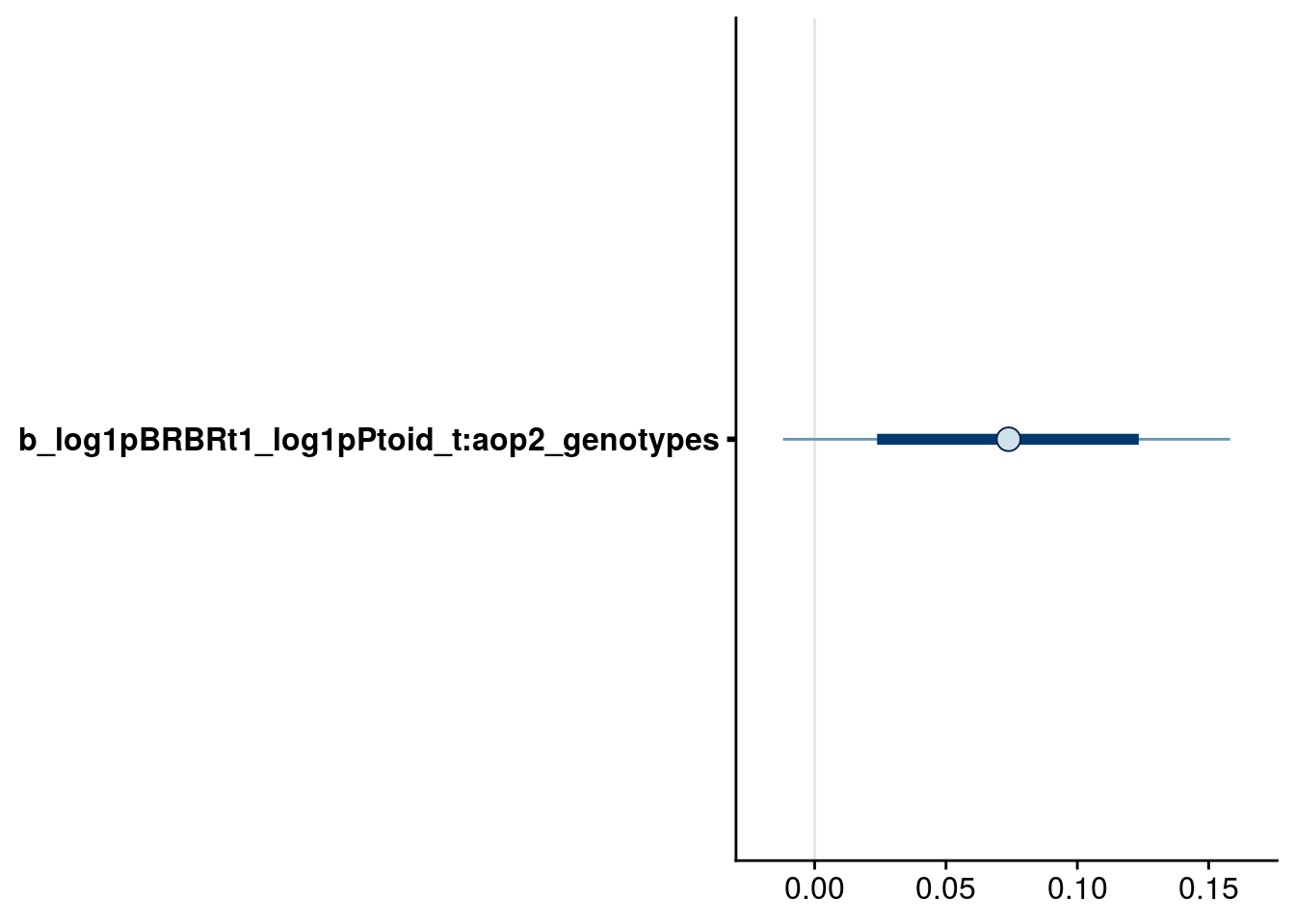
This is still an intermediate model because not all terms meet our 90% criteria.
Reduced model 4
Drop terms
Based on the above plots, I dropped the following terms:
Effects on BRBR_t1:
log1p(Ptoid_t):aop2_genotypes
Effects on LYER_t1:
- keep all
Effects on Ptoid_t1:
- keep all
Refit model
# update formulas
reduced.4.BRBR.bf <- update(reduced.3.BRBR.bf, .~. -log1p(Ptoid_t):aop2_genotypes -log1p(Ptoid_t):AOP2_genotypes)
reduced.4.LYER.bf <- reduced.3.LYER.bf
reduced.4.Ptoid.bf <- reduced.3.Ptoid.bf

# fit new model
reduced.4.brm <- brm(
  data = full_df,
  formula = mvbf(reduced.4.BRBR.bf, reduced.4.LYER.bf, reduced.4.Ptoid.bf),
  iter = 4000,
  prior = c(# growth rates
            set_prior(prior.r.BRBR, class = "b", coef = "intercept", resp = "log1pBRBRt1"),
            set_prior(prior.r.LYER, class = "b", coef = "intercept", resp = "log1pLYERt1"),
            set_prior(prior.r.Ptoid, class = "b", coef = "intercept", resp = "log1pPtoidt1"),
            # intraspecific effects
            #set_prior(prior.intra.BRBR, class = "b", coef = "log1pBRBR_t", resp = "log1pBRBRt1"),
            set_prior(prior.intra.LYER, class = "b", coef = "log1pLYER_t", resp = "log1pLYERt1"),
            #set_prior(prior.intra.LYER, class = "b", coef = "log1pPtoid_t", resp = "log1pPtoidt1"),
            # negative interspecific effects
            #set_prior(prior.LYERonBRBR, class = "b", coef = "log1pLYER_t", resp = "log1pBRBRt1"),
            set_prior(prior.BRBRonLYER, class = "b", coef = "log1pBRBR_t", resp = "log1pLYERt1"),
            set_prior(prior.PtoidonBRBR, class = "b", coef = "log1pPtoid_t", resp = "log1pBRBRt1"),
            set_prior(prior.PtoidonLYER, class = "b", coef = "log1pPtoid_t", resp = "log1pLYERt1"),
            # positive interspecific effects
            set_prior(prior.BRBRonPtoid, class = "b", coef = "log1pBRBR_t", resp = "log1pPtoidt1"),
            set_prior(prior.LYERonPtoid, class = "b", coef = "log1pLYER_t", resp = "log1pPtoidt1"),
            # aop2 effects
            set_prior(prior.rich, class = "b", coef = "aop2_genotypes", resp = "log1pBRBRt1"),
            set_prior(prior.rich, class = "b", coef = "aop2_genotypes", resp = "log1pLYERt1"),
            set_prior(prior.rich, class = "b", coef = "aop2_genotypes", resp = "log1pPtoidt1"),
            #set_prior(prior.rich, class = "b", coef = "log1pBRBR_t:aop2_genotypes", resp = "log1pBRBRt1"),
            #set_prior(prior.rich, class = "b", coef = "log1pBRBR_t:aop2_genotypes", resp = "log1pLYERt1"),
            #set_prior(prior.rich, class = "b", coef = "log1pBRBR_t:aop2_genotypes", resp = "log1pPtoidt1"),
            #set_prior(prior.rich, class = "b", coef = "log1pLYER_t:aop2_genotypes", resp = "log1pBRBRt1"),
            #set_prior(prior.rich, class = "b", coef = "log1pLYER_t:aop2_genotypes", resp = "log1pLYERt1"),
            #set_prior(prior.rich, class = "b", coef = "log1pLYER_t:aop2_genotypes", resp = "log1pPtoidt1"),
            #set_prior(prior.rich, class = "b", coef = "log1pPtoid_t:aop2_genotypes", resp = "log1pBRBRt1"),
            #set_prior(prior.rich, class = "b", coef = "log1pPtoid_t:aop2_genotypes", resp = "log1pLYERt1"),
            #set_prior(prior.rich, class = "b", coef = "log1pPtoid_t:aop2_genotypes", resp = "log1pPtoidt1"),
            # AOP2 effects
            set_prior(prior.rich, class = "b", coef = "AOP2_genotypes", resp = "log1pBRBRt1"),
            set_prior(prior.rich, class = "b", coef = "AOP2_genotypes", resp = "log1pLYERt1"),
            set_prior(prior.rich, class = "b", coef = "AOP2_genotypes", resp = "log1pPtoidt1"),
            #set_prior(prior.rich, class = "b", coef = "log1pBRBR_t:AOP2_genotypes", resp = "log1pBRBRt1"),
            #set_prior(prior.rich, class = "b", coef = "log1pBRBR_t:AOP2_genotypes", resp = "log1pLYERt1"),
            #set_prior(prior.rich, class = "b", coef = "log1pBRBR_t:AOP2_genotypes", resp = "log1pPtoidt1"),
            #set_prior(prior.rich, class = "b", coef = "log1pLYER_t:AOP2_genotypes", resp = "log1pBRBRt1"),
            #set_prior(prior.rich, class = "b", coef = "log1pLYER_t:AOP2_genotypes", resp = "log1pLYERt1"),
            #set_prior(prior.rich, class = "b", coef = "log1pLYER_t:AOP2_genotypes", resp = "log1pPtoidt1"),
            #set_prior(prior.rich, class = "b", coef = "log1pPtoid_t:AOP2_genotypes", resp = "log1pBRBRt1"),
            #set_prior(prior.rich, class = "b", coef = "log1pPtoid_t:AOP2_genotypes", resp = "log1pLYERt1"),
            #set_prior(prior.rich, class = "b", coef = "log1pPtoid_t:AOP2_genotypes", resp = "log1pPtoidt1"),
            # temp effects
            set_prior(prior.temp, class = "b", coef = "temp", resp = "log1pBRBRt1"),
            #set_prior(prior.temp, class = "b", coef = "temp", resp = "log1pLYERt1"),
            set_prior(prior.temp, class = "b", coef = "temp", resp = "log1pPtoidt1"),
            #set_prior(prior.temp, class = "b", coef = "log1pBRBR_t:temp", resp = "log1pBRBRt1"),
            #set_prior(prior.temp, class = "b", coef = "log1pBRBR_t:temp", resp = "log1pLYERt1"),
            set_prior(prior.temp, class = "b", coef = "log1pBRBR_t:temp", resp = "log1pPtoidt1"),
            #set_prior(prior.temp, class = "b", coef = "log1pLYER_t:temp", resp = "log1pBRBRt1"),
            #set_prior(prior.temp, class = "b", coef = "log1pLYER_t:temp", resp = "log1pLYERt1"),
            #set_prior(prior.temp, class = "b", coef = "log1pLYER_t:temp", resp = "log1pPtoidt1"),
            set_prior(prior.temp, class = "b", coef = "log1pPtoid_t:temp", resp = "log1pBRBRt1"),
            #set_prior(prior.temp, class = "b", coef = "log1pPtoid_t:temp", resp = "log1pLYERt1"),
            #set_prior(prior.temp, class = "b", coef = "log1pPtoid_t:temp", resp = "log1pPtoidt1"),
            # biomass effects
            #set_prior(prior.AphidBiomass, class = "b", coef = "logBiomass_g_t1", resp = "log1pBRBRt1"),
            #set_prior(prior.AphidBiomass, class = "b", coef = "logBiomass_g_t1", resp = "log1pLYERt1"),
            set_prior(prior.PtoidBiomass, class = "b", coef = "logBiomass_g_t1", resp = "log1pPtoidt1"),
            # random effects
            set_prior(prior.random.effects, class = "sd", resp = "log1pBRBRt1"),
            set_prior(prior.random.effects, class = "sd", resp = "log1pLYERt1"),
            set_prior(prior.random.effects, class = "sd", resp = "log1pPtoidt1")),
  file = "output/reduced.4.brm.keystone.rds")

# print model summary
summary(reduced.4.brm)
Family: MV(gaussian, gaussian, gaussian)
Links: mu = identity; sigma = identity
mu = identity; sigma = identity
mu = identity; sigma = identity
Formula: log1p(BRBR_t1) ~ intercept + log1p(Ptoid_t) + temp + aop2_genotypes + AOP2_genotypes + (1 | Cage) + ar(time = Week_match.1p, gr = Cage, p = 1, cov = FALSE) + log1p(Ptoid_t):temp + offset(log1p(BRBR_t)) - 1
log1p(LYER_t1) ~ intercept + log1p(BRBR_t) + log1p(LYER_t) + log1p(Ptoid_t) + aop2_genotypes + AOP2_genotypes + (1 | Cage) + ar(time = Week_match.1p, gr = Cage, p = 1, cov = FALSE) + offset(log1p(LYER_t)) - 1
log1p(Ptoid_t1) ~ intercept + log1p(BRBR_t) + log1p(LYER_t) + temp + aop2_genotypes + AOP2_genotypes + log(Biomass_g_t1) + (1 | Cage) + ar(time = Week_match.1p, gr = Cage, p = 1, cov = FALSE) + log1p(BRBR_t):temp + offset(log1p(Ptoid_t)) - 1
Data: full_df (Number of observations: 264)
Samples: 4 chains, each with iter = 4000; warmup = 2000; thin = 1;
total post-warmup samples = 8000
Correlation Structures:
Estimate Est.Error l-95% CI u-95% CI Rhat Bulk_ESS Tail_ESS
ar_log1pBRBRt1[1] -0.43 0.09 -0.61 -0.26 1.00 2702 4557
ar_log1pLYERt1[1] -0.10 0.10 -0.28 0.10 1.00 4647 5689
ar_log1pPtoidt1[1] -0.49 0.08 -0.65 -0.33 1.00 6850 6068
Group-Level Effects:
~Cage (Number of levels: 60)
Estimate Est.Error l-95% CI u-95% CI Rhat Bulk_ESS
sd(log1pBRBRt1_Intercept) 0.26 0.10 0.04 0.44 1.00 1062
sd(log1pLYERt1_Intercept) 0.13 0.08 0.01 0.31 1.00 1621
sd(log1pPtoidt1_Intercept) 0.04 0.03 0.00 0.11 1.00 3903
Tail_ESS
sd(log1pBRBRt1_Intercept) 1121
sd(log1pLYERt1_Intercept) 2399
sd(log1pPtoidt1_Intercept) 3149
Population-Level Effects:
Estimate Est.Error l-95% CI u-95% CI Rhat
log1pBRBRt1_intercept 1.62 0.21 1.22 2.05 1.00
log1pBRBRt1_log1pPtoid_t -0.91 0.05 -1.01 -0.80 1.00
log1pBRBRt1_temp -0.71 0.08 -0.86 -0.56 1.00
log1pBRBRt1_aop2_genotypes 0.04 0.09 -0.15 0.22 1.00
log1pBRBRt1_AOP2_genotypes -0.01 0.09 -0.18 0.16 1.00
log1pBRBRt1_log1pPtoid_t:temp 0.17 0.03 0.11 0.23 1.00
log1pLYERt1_intercept 3.46 0.45 2.58 4.36 1.00
log1pLYERt1_log1pBRBR_t 0.23 0.05 0.12 0.33 1.00
log1pLYERt1_log1pLYER_t -0.66 0.08 -0.82 -0.50 1.00
log1pLYERt1_log1pPtoid_t -0.72 0.05 -0.82 -0.62 1.00
log1pLYERt1_aop2_genotypes 0.20 0.08 0.04 0.37 1.00
log1pLYERt1_AOP2_genotypes -0.08 0.08 -0.24 0.08 1.00
log1pPtoidt1_intercept -2.89 0.38 -3.65 -2.16 1.00
log1pPtoidt1_log1pBRBR_t 0.35 0.06 0.23 0.48 1.00
log1pPtoidt1_log1pLYER_t 0.35 0.06 0.22 0.48 1.00
log1pPtoidt1_temp 0.67 0.12 0.44 0.90 1.00
log1pPtoidt1_aop2_genotypes 0.11 0.06 -0.02 0.23 1.00
log1pPtoidt1_AOP2_genotypes -0.08 0.06 -0.19 0.03 1.00
log1pPtoidt1_logBiomass_g_t1 -0.72 0.17 -1.06 -0.39 1.00
log1pPtoidt1_log1pBRBR_t:temp -0.17 0.02 -0.22 -0.12 1.00
Bulk_ESS Tail_ESS
log1pBRBRt1_intercept 3444 4225
log1pBRBRt1_log1pPtoid_t 3868 4922
log1pBRBRt1_temp 4252 4630
log1pBRBRt1_aop2_genotypes 4631 4990
log1pBRBRt1_AOP2_genotypes 4932 5592
log1pBRBRt1_log1pPtoid_t:temp 4972 5121
log1pLYERt1_intercept 3889 4763
log1pLYERt1_log1pBRBR_t 4957 5715
log1pLYERt1_log1pLYER_t 3270 3814
log1pLYERt1_log1pPtoid_t 4256 4865
log1pLYERt1_aop2_genotypes 6445 5580
log1pLYERt1_AOP2_genotypes 6817 6491
log1pPtoidt1_intercept 3133 4611
log1pPtoidt1_log1pBRBR_t 3936 4783
log1pPtoidt1_log1pLYER_t 5082 5460
log1pPtoidt1_temp 3413 4651
log1pPtoidt1_aop2_genotypes 5411 5549
log1pPtoidt1_AOP2_genotypes 5701 6162
log1pPtoidt1_logBiomass_g_t1 4225 4641
log1pPtoidt1_log1pBRBR_t:temp 3641 5206
Family Specific Parameters:
Estimate Est.Error l-95% CI u-95% CI Rhat Bulk_ESS Tail_ESS
sigma_log1pBRBRt1 1.12 0.06 1.01 1.24 1.00 3045 5241
sigma_log1pLYERt1 0.92 0.04 0.84 1.01 1.00 5976 6022
sigma_log1pPtoidt1 0.76 0.03 0.70 0.83 1.00 9296 6248
Residual Correlations:
Estimate Est.Error l-95% CI u-95% CI Rhat
rescor(log1pBRBRt1,log1pLYERt1) 0.53 0.05 0.43 0.62 1.00
rescor(log1pBRBRt1,log1pPtoidt1) -0.03 0.07 -0.18 0.10 1.00
rescor(log1pLYERt1,log1pPtoidt1) 0.05 0.06 -0.07 0.18 1.00
Bulk_ESS Tail_ESS
rescor(log1pBRBRt1,log1pLYERt1) 6477 6412
rescor(log1pBRBRt1,log1pPtoidt1) 5985 5627
rescor(log1pLYERt1,log1pPtoidt1) 9611 6499
Samples were drawn using sampling(NUTS). For each parameter, Bulk_ESS
and Tail_ESS are effective sample size measures, and Rhat is the potential
scale reduction factor on split chains (at convergence, Rhat = 1).Inspect credible intervals
# check aop2 effects on growth rates
bayesplot::mcmc_intervals(reduced.4.brm, regex_pars = "_aop2_genotypes$", prob = 0.66, prob_outer = 0.90) # drop aop2 effect on BRBR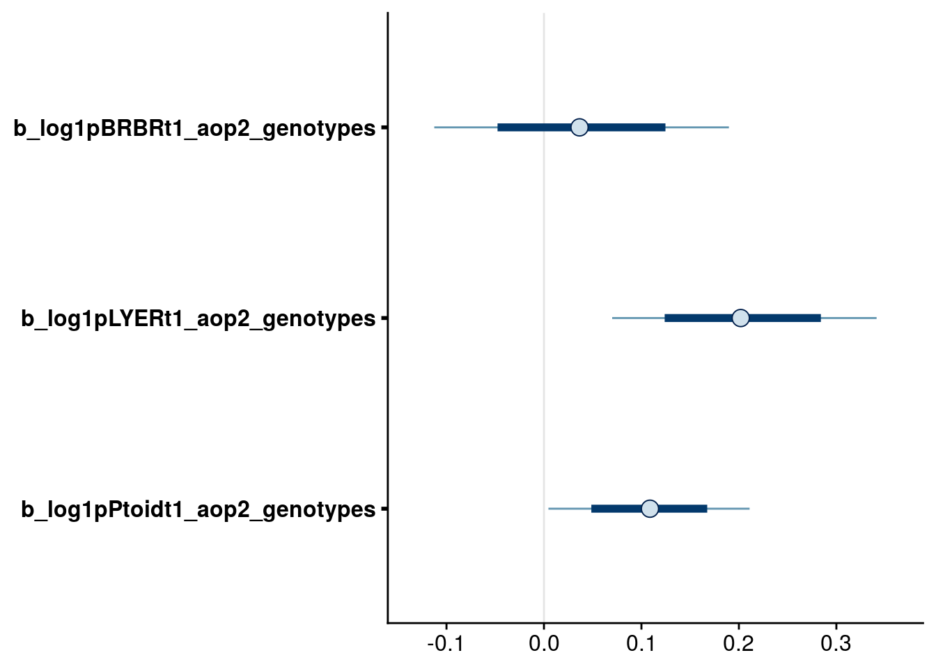
Again, this model is still an intermediate one because not all terms meet the 90% criteria.
Reduced model 5
Drop terms
Based on the above plots, I dropped the following terms:
Effects on BRBR_t1:
aop2_genotypes
Effects on LYER_t1:
- keep all
Effects on Ptoid_t1:
- keep all
Refit model
# update formulas
reduced.5.BRBR.bf <- update(reduced.4.BRBR.bf, .~. -aop2_genotypes -AOP2_genotypes)
reduced.5.LYER.bf <- reduced.4.LYER.bf
reduced.5.Ptoid.bf <- reduced.4.Ptoid.bf

# fit new model
reduced.5.brm <- brm(
  data = full_df,
  formula = mvbf(reduced.5.BRBR.bf, reduced.5.LYER.bf, reduced.5.Ptoid.bf),
  iter = 4000,
  prior = c(# growth rates
            set_prior(prior.r.BRBR, class = "b", coef = "intercept", resp = "log1pBRBRt1"),
            set_prior(prior.r.LYER, class = "b", coef = "intercept", resp = "log1pLYERt1"),
            set_prior(prior.r.Ptoid, class = "b", coef = "intercept", resp = "log1pPtoidt1"),
            # intraspecific effects
            #set_prior(prior.intra.BRBR, class = "b", coef = "log1pBRBR_t", resp = "log1pBRBRt1"),
            set_prior(prior.intra.LYER, class = "b", coef = "log1pLYER_t", resp = "log1pLYERt1"),
            #set_prior(prior.intra.LYER, class = "b", coef = "log1pPtoid_t", resp = "log1pPtoidt1"),
            # negative interspecific effects
            #set_prior(prior.LYERonBRBR, class = "b", coef = "log1pLYER_t", resp = "log1pBRBRt1"),
            set_prior(prior.BRBRonLYER, class = "b", coef = "log1pBRBR_t", resp = "log1pLYERt1"),
            set_prior(prior.PtoidonBRBR, class = "b", coef = "log1pPtoid_t", resp = "log1pBRBRt1"),
            set_prior(prior.PtoidonLYER, class = "b", coef = "log1pPtoid_t", resp = "log1pLYERt1"),
            # positive interspecific effects
            set_prior(prior.BRBRonPtoid, class = "b", coef = "log1pBRBR_t", resp = "log1pPtoidt1"),
            set_prior(prior.LYERonPtoid, class = "b", coef = "log1pLYER_t", resp = "log1pPtoidt1"),
            # aop2 effects
            #set_prior(prior.rich, class = "b", coef = "aop2_genotypes", resp = "log1pBRBRt1"),
            set_prior(prior.rich, class = "b", coef = "aop2_genotypes", resp = "log1pLYERt1"),
            set_prior(prior.rich, class = "b", coef = "aop2_genotypes", resp = "log1pPtoidt1"),
            #set_prior(prior.rich, class = "b", coef = "log1pBRBR_t:aop2_genotypes", resp = "log1pBRBRt1"),
            #set_prior(prior.rich, class = "b", coef = "log1pBRBR_t:aop2_genotypes", resp = "log1pLYERt1"),
            #set_prior(prior.rich, class = "b", coef = "log1pBRBR_t:aop2_genotypes", resp = "log1pPtoidt1"),
            #set_prior(prior.rich, class = "b", coef = "log1pLYER_t:aop2_genotypes", resp = "log1pBRBRt1"),
            #set_prior(prior.rich, class = "b", coef = "log1pLYER_t:aop2_genotypes", resp = "log1pLYERt1"),
            #set_prior(prior.rich, class = "b", coef = "log1pLYER_t:aop2_genotypes", resp = "log1pPtoidt1"),
            #set_prior(prior.rich, class = "b", coef = "log1pPtoid_t:aop2_genotypes", resp = "log1pBRBRt1"),
            #set_prior(prior.rich, class = "b", coef = "log1pPtoid_t:aop2_genotypes", resp = "log1pLYERt1"),
            #set_prior(prior.rich, class = "b", coef = "log1pPtoid_t:aop2_genotypes", resp = "log1pPtoidt1"),
            # AOP2 effects
            #set_prior(prior.rich, class = "b", coef = "AOP2_genotypes", resp = "log1pBRBRt1"),
            set_prior(prior.rich, class = "b", coef = "AOP2_genotypes", resp = "log1pLYERt1"),
            set_prior(prior.rich, class = "b", coef = "AOP2_genotypes", resp = "log1pPtoidt1"),
            #set_prior(prior.rich, class = "b", coef = "log1pBRBR_t:AOP2_genotypes", resp = "log1pBRBRt1"),
            #set_prior(prior.rich, class = "b", coef = "log1pBRBR_t:AOP2_genotypes", resp = "log1pLYERt1"),
            #set_prior(prior.rich, class = "b", coef = "log1pBRBR_t:AOP2_genotypes", resp = "log1pPtoidt1"),
            #set_prior(prior.rich, class = "b", coef = "log1pLYER_t:AOP2_genotypes", resp = "log1pBRBRt1"),
            #set_prior(prior.rich, class = "b", coef = "log1pLYER_t:AOP2_genotypes", resp = "log1pLYERt1"),
            #set_prior(prior.rich, class = "b", coef = "log1pLYER_t:AOP2_genotypes", resp = "log1pPtoidt1"),
            #set_prior(prior.rich, class = "b", coef = "log1pPtoid_t:AOP2_genotypes", resp = "log1pBRBRt1"),
            #set_prior(prior.rich, class = "b", coef = "log1pPtoid_t:AOP2_genotypes", resp = "log1pLYERt1"),
            #set_prior(prior.rich, class = "b", coef = "log1pPtoid_t:AOP2_genotypes", resp = "log1pPtoidt1"),
            # temp effects
            set_prior(prior.temp, class = "b", coef = "temp", resp = "log1pBRBRt1"),
            #set_prior(prior.temp, class = "b", coef = "temp", resp = "log1pLYERt1"),
            set_prior(prior.temp, class = "b", coef = "temp", resp = "log1pPtoidt1"),
            #set_prior(prior.temp, class = "b", coef = "log1pBRBR_t:temp", resp = "log1pBRBRt1"),
            #set_prior(prior.temp, class = "b", coef = "log1pBRBR_t:temp", resp = "log1pLYERt1"),
            set_prior(prior.temp, class = "b", coef = "log1pBRBR_t:temp", resp = "log1pPtoidt1"),
            #set_prior(prior.temp, class = "b", coef = "log1pLYER_t:temp", resp = "log1pBRBRt1"),
            #set_prior(prior.temp, class = "b", coef = "log1pLYER_t:temp", resp = "log1pLYERt1"),
            #set_prior(prior.temp, class = "b", coef = "log1pLYER_t:temp", resp = "log1pPtoidt1"),
            set_prior(prior.temp, class = "b", coef = "log1pPtoid_t:temp", resp = "log1pBRBRt1"),
            #set_prior(prior.temp, class = "b", coef = "log1pPtoid_t:temp", resp = "log1pLYERt1"),
            #set_prior(prior.temp, class = "b", coef = "log1pPtoid_t:temp", resp = "log1pPtoidt1"),
            # biomass effects
            #set_prior(prior.AphidBiomass, class = "b", coef = "logBiomass_g_t1", resp = "log1pBRBRt1"),
            #set_prior(prior.AphidBiomass, class = "b", coef = "logBiomass_g_t1", resp = "log1pLYERt1"),
            set_prior(prior.PtoidBiomass, class = "b", coef = "logBiomass_g_t1", resp = "log1pPtoidt1"),
            # random effects
            set_prior(prior.random.effects, class = "sd", resp = "log1pBRBRt1"),
            set_prior(prior.random.effects, class = "sd", resp = "log1pLYERt1"),
            set_prior(prior.random.effects, class = "sd", resp = "log1pPtoidt1")),
  file = "output/reduced.5.brm.keystone.rds")

# print model summary
summary(reduced.5.brm)
Family: MV(gaussian, gaussian, gaussian)
Links: mu = identity; sigma = identity
mu = identity; sigma = identity
mu = identity; sigma = identity
Formula: log1p(BRBR_t1) ~ intercept + log1p(Ptoid_t) + temp + (1 | Cage) + ar(time = Week_match.1p, gr = Cage, p = 1, cov = FALSE) + log1p(Ptoid_t):temp + offset(log1p(BRBR_t)) - 1
log1p(LYER_t1) ~ intercept + log1p(BRBR_t) + log1p(LYER_t) + log1p(Ptoid_t) + aop2_genotypes + AOP2_genotypes + (1 | Cage) + ar(time = Week_match.1p, gr = Cage, p = 1, cov = FALSE) + offset(log1p(LYER_t)) - 1
log1p(Ptoid_t1) ~ intercept + log1p(BRBR_t) + log1p(LYER_t) + temp + aop2_genotypes + AOP2_genotypes + log(Biomass_g_t1) + (1 | Cage) + ar(time = Week_match.1p, gr = Cage, p = 1, cov = FALSE) + log1p(BRBR_t):temp + offset(log1p(Ptoid_t)) - 1
Data: full_df (Number of observations: 264)
Samples: 4 chains, each with iter = 4000; warmup = 2000; thin = 1;
total post-warmup samples = 8000
Correlation Structures:
Estimate Est.Error l-95% CI u-95% CI Rhat Bulk_ESS Tail_ESS
ar_log1pBRBRt1[1] -0.43 0.09 -0.60 -0.25 1.00 2966 4900
ar_log1pLYERt1[1] -0.10 0.09 -0.28 0.09 1.00 3993 5073
ar_log1pPtoidt1[1] -0.50 0.08 -0.65 -0.33 1.00 7256 6067
Group-Level Effects:
~Cage (Number of levels: 60)
Estimate Est.Error l-95% CI u-95% CI Rhat Bulk_ESS
sd(log1pBRBRt1_Intercept) 0.24 0.10 0.03 0.42 1.00 1060
sd(log1pLYERt1_Intercept) 0.13 0.08 0.01 0.31 1.00 1476
sd(log1pPtoidt1_Intercept) 0.04 0.03 0.00 0.11 1.00 4300
Tail_ESS
sd(log1pBRBRt1_Intercept) 1646
sd(log1pLYERt1_Intercept) 2398
sd(log1pPtoidt1_Intercept) 3639
Population-Level Effects:
Estimate Est.Error l-95% CI u-95% CI Rhat
log1pBRBRt1_intercept 1.65 0.16 1.33 1.96 1.00
log1pBRBRt1_log1pPtoid_t -0.90 0.05 -1.00 -0.80 1.00
log1pBRBRt1_temp -0.70 0.08 -0.86 -0.56 1.00
log1pBRBRt1_log1pPtoid_t:temp 0.17 0.03 0.11 0.22 1.00
log1pLYERt1_intercept 3.48 0.46 2.59 4.38 1.00
log1pLYERt1_log1pBRBR_t 0.23 0.05 0.12 0.34 1.00
log1pLYERt1_log1pLYER_t -0.66 0.08 -0.82 -0.50 1.00
log1pLYERt1_log1pPtoid_t -0.72 0.05 -0.82 -0.62 1.00
log1pLYERt1_aop2_genotypes 0.19 0.08 0.04 0.34 1.00
log1pLYERt1_AOP2_genotypes -0.08 0.07 -0.22 0.07 1.00
log1pPtoidt1_intercept -2.89 0.39 -3.65 -2.14 1.00
log1pPtoidt1_log1pBRBR_t 0.35 0.06 0.23 0.47 1.00
log1pPtoidt1_log1pLYER_t 0.35 0.06 0.23 0.48 1.00
log1pPtoidt1_temp 0.67 0.12 0.44 0.89 1.00
log1pPtoidt1_aop2_genotypes 0.11 0.06 -0.02 0.24 1.00
log1pPtoidt1_AOP2_genotypes -0.08 0.06 -0.19 0.03 1.00
log1pPtoidt1_logBiomass_g_t1 -0.72 0.17 -1.05 -0.39 1.00
log1pPtoidt1_log1pBRBR_t:temp -0.17 0.02 -0.22 -0.12 1.00
Bulk_ESS Tail_ESS
log1pBRBRt1_intercept 3211 5020
log1pBRBRt1_log1pPtoid_t 2994 5018
log1pBRBRt1_temp 3830 5069
log1pBRBRt1_log1pPtoid_t:temp 4287 5481
log1pLYERt1_intercept 3845 5019
log1pLYERt1_log1pBRBR_t 5273 5250
log1pLYERt1_log1pLYER_t 3512 4369
log1pLYERt1_log1pPtoid_t 4063 4867
log1pLYERt1_aop2_genotypes 6884 6090
log1pLYERt1_AOP2_genotypes 7173 6224
log1pPtoidt1_intercept 3774 4961
log1pPtoidt1_log1pBRBR_t 3767 5311
log1pPtoidt1_log1pLYER_t 5302 5846
log1pPtoidt1_temp 3292 4569
log1pPtoidt1_aop2_genotypes 5728 5884
log1pPtoidt1_AOP2_genotypes 6122 6041
log1pPtoidt1_logBiomass_g_t1 4707 5635
log1pPtoidt1_log1pBRBR_t:temp 3672 5118
Family Specific Parameters:
Estimate Est.Error l-95% CI u-95% CI Rhat Bulk_ESS Tail_ESS
sigma_log1pBRBRt1 1.12 0.06 1.02 1.24 1.00 2575 4739
sigma_log1pLYERt1 0.92 0.04 0.84 1.01 1.00 5398 5315
sigma_log1pPtoidt1 0.76 0.03 0.70 0.83 1.00 9242 5156
Residual Correlations:
Estimate Est.Error l-95% CI u-95% CI Rhat
rescor(log1pBRBRt1,log1pLYERt1) 0.53 0.05 0.43 0.62 1.00
rescor(log1pBRBRt1,log1pPtoidt1) -0.03 0.07 -0.17 0.11 1.00
rescor(log1pLYERt1,log1pPtoidt1) 0.05 0.06 -0.07 0.18 1.00
Bulk_ESS Tail_ESS
rescor(log1pBRBRt1,log1pLYERt1) 5770 5034
rescor(log1pBRBRt1,log1pPtoidt1) 6362 5950
rescor(log1pLYERt1,log1pPtoidt1) 7912 6294
Samples were drawn using sampling(NUTS). For each parameter, Bulk_ESS
and Tail_ESS are effective sample size measures, and Rhat is the potential
scale reduction factor on split chains (at convergence, Rhat = 1).Inspect credible intervals
# no more higher-order terms, so check aop2 effects on growth rates
bayesplot::mcmc_intervals(reduced.5.brm, regex_pars = "_aop2_genotypes$", prob = 0.66, prob_outer = 0.90) 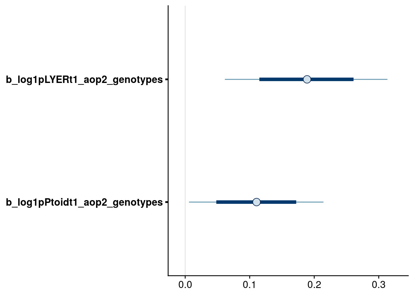
Now, we have a model where all terms meet our 90% criteria. Let’s evaluate it’s effect on LYER-Ptoid persistence.
pp_aop2_LP_persist(reduced.5.brm, temp.cond = 1.5, aop2.cond = 2)aop2_LPbound_BayesP aop2_LPbound_effect
0.999500 8.399152 There is clear evidence that AOP2\(-\) promotes LYER-Ptoid persistence relative to AOP2\(+\) in this model.
Reduced model 6
What about a model where we use a 95% cutoff?
bayesplot::mcmc_intervals(reduced.5.brm, regex_pars = "_aop2_genotypes$", prob = 0.66, prob_outer = 0.95) # suggest dropping aop2 effect on Ptoid.
Drop terms
Based on the above plots, I dropped the following terms:
Effects on BRBR_t1:
- keep all
Effects on LYER_t1:
- keep all
Effects on Ptoid_t1:
aop2_genotypes
Refit model
# update formulas
reduced.6.BRBR.bf <- reduced.5.BRBR.bf
reduced.6.LYER.bf <- reduced.5.LYER.bf
reduced.6.Ptoid.bf <- update(reduced.5.Ptoid.bf, .~. -aop2_genotypes -AOP2_genotypes)

# fit new model
reduced.6.brm <- brm(
  data = full_df,
  formula = mvbf(reduced.6.BRBR.bf, reduced.6.LYER.bf, reduced.6.Ptoid.bf),
  iter = 4000,
  prior = c(# growth rates
            set_prior(prior.r.BRBR, class = "b", coef = "intercept", resp = "log1pBRBRt1"),
            set_prior(prior.r.LYER, class = "b", coef = "intercept", resp = "log1pLYERt1"),
            set_prior(prior.r.Ptoid, class = "b", coef = "intercept", resp = "log1pPtoidt1"),
            # intraspecific effects
            #set_prior(prior.intra.BRBR, class = "b", coef = "log1pBRBR_t", resp = "log1pBRBRt1"),
            set_prior(prior.intra.LYER, class = "b", coef = "log1pLYER_t", resp = "log1pLYERt1"),
            #set_prior(prior.intra.LYER, class = "b", coef = "log1pPtoid_t", resp = "log1pPtoidt1"),
            # negative interspecific effects
            #set_prior(prior.LYERonBRBR, class = "b", coef = "log1pLYER_t", resp = "log1pBRBRt1"),
            set_prior(prior.BRBRonLYER, class = "b", coef = "log1pBRBR_t", resp = "log1pLYERt1"),
            set_prior(prior.PtoidonBRBR, class = "b", coef = "log1pPtoid_t", resp = "log1pBRBRt1"),
            set_prior(prior.PtoidonLYER, class = "b", coef = "log1pPtoid_t", resp = "log1pLYERt1"),
            # positive interspecific effects
            set_prior(prior.BRBRonPtoid, class = "b", coef = "log1pBRBR_t", resp = "log1pPtoidt1"),
            set_prior(prior.LYERonPtoid, class = "b", coef = "log1pLYER_t", resp = "log1pPtoidt1"),
            # aop2 effects
            #set_prior(prior.rich, class = "b", coef = "aop2_genotypes", resp = "log1pBRBRt1"),
            set_prior(prior.rich, class = "b", coef = "aop2_genotypes", resp = "log1pLYERt1"),
            #set_prior(prior.rich, class = "b", coef = "aop2_genotypes", resp = "log1pPtoidt1"),
            #set_prior(prior.rich, class = "b", coef = "log1pBRBR_t:aop2_genotypes", resp = "log1pBRBRt1"),
            #set_prior(prior.rich, class = "b", coef = "log1pBRBR_t:aop2_genotypes", resp = "log1pLYERt1"),
            #set_prior(prior.rich, class = "b", coef = "log1pBRBR_t:aop2_genotypes", resp = "log1pPtoidt1"),
            #set_prior(prior.rich, class = "b", coef = "log1pLYER_t:aop2_genotypes", resp = "log1pBRBRt1"),
            #set_prior(prior.rich, class = "b", coef = "log1pLYER_t:aop2_genotypes", resp = "log1pLYERt1"),
            #set_prior(prior.rich, class = "b", coef = "log1pLYER_t:aop2_genotypes", resp = "log1pPtoidt1"),
            #set_prior(prior.rich, class = "b", coef = "log1pPtoid_t:aop2_genotypes", resp = "log1pBRBRt1"),
            #set_prior(prior.rich, class = "b", coef = "log1pPtoid_t:aop2_genotypes", resp = "log1pLYERt1"),
            #set_prior(prior.rich, class = "b", coef = "log1pPtoid_t:aop2_genotypes", resp = "log1pPtoidt1"),
            # AOP2 effects
            #set_prior(prior.rich, class = "b", coef = "AOP2_genotypes", resp = "log1pBRBRt1"),
            set_prior(prior.rich, class = "b", coef = "AOP2_genotypes", resp = "log1pLYERt1"),
            #set_prior(prior.rich, class = "b", coef = "AOP2_genotypes", resp = "log1pPtoidt1"),
            #set_prior(prior.rich, class = "b", coef = "log1pBRBR_t:AOP2_genotypes", resp = "log1pBRBRt1"),
            #set_prior(prior.rich, class = "b", coef = "log1pBRBR_t:AOP2_genotypes", resp = "log1pLYERt1"),
            #set_prior(prior.rich, class = "b", coef = "log1pBRBR_t:AOP2_genotypes", resp = "log1pPtoidt1"),
            #set_prior(prior.rich, class = "b", coef = "log1pLYER_t:AOP2_genotypes", resp = "log1pBRBRt1"),
            #set_prior(prior.rich, class = "b", coef = "log1pLYER_t:AOP2_genotypes", resp = "log1pLYERt1"),
            #set_prior(prior.rich, class = "b", coef = "log1pLYER_t:AOP2_genotypes", resp = "log1pPtoidt1"),
            #set_prior(prior.rich, class = "b", coef = "log1pPtoid_t:AOP2_genotypes", resp = "log1pBRBRt1"),
            #set_prior(prior.rich, class = "b", coef = "log1pPtoid_t:AOP2_genotypes", resp = "log1pLYERt1"),
            #set_prior(prior.rich, class = "b", coef = "log1pPtoid_t:AOP2_genotypes", resp = "log1pPtoidt1"),
            # temp effects
            set_prior(prior.temp, class = "b", coef = "temp", resp = "log1pBRBRt1"),
            #set_prior(prior.temp, class = "b", coef = "temp", resp = "log1pLYERt1"),
            set_prior(prior.temp, class = "b", coef = "temp", resp = "log1pPtoidt1"),
            #set_prior(prior.temp, class = "b", coef = "log1pBRBR_t:temp", resp = "log1pBRBRt1"),
            #set_prior(prior.temp, class = "b", coef = "log1pBRBR_t:temp", resp = "log1pLYERt1"),
            set_prior(prior.temp, class = "b", coef = "log1pBRBR_t:temp", resp = "log1pPtoidt1"),
            #set_prior(prior.temp, class = "b", coef = "log1pLYER_t:temp", resp = "log1pBRBRt1"),
            #set_prior(prior.temp, class = "b", coef = "log1pLYER_t:temp", resp = "log1pLYERt1"),
            #set_prior(prior.temp, class = "b", coef = "log1pLYER_t:temp", resp = "log1pPtoidt1"),
            set_prior(prior.temp, class = "b", coef = "log1pPtoid_t:temp", resp = "log1pBRBRt1"),
            #set_prior(prior.temp, class = "b", coef = "log1pPtoid_t:temp", resp = "log1pLYERt1"),
            #set_prior(prior.temp, class = "b", coef = "log1pPtoid_t:temp", resp = "log1pPtoidt1"),
            # biomass effects
            #set_prior(prior.AphidBiomass, class = "b", coef = "logBiomass_g_t1", resp = "log1pBRBRt1"),
            #set_prior(prior.AphidBiomass, class = "b", coef = "logBiomass_g_t1", resp = "log1pLYERt1"),
            set_prior(prior.PtoidBiomass, class = "b", coef = "logBiomass_g_t1", resp = "log1pPtoidt1"),
            # random effects
            set_prior(prior.random.effects, class = "sd", resp = "log1pBRBRt1"),
            set_prior(prior.random.effects, class = "sd", resp = "log1pLYERt1"),
            set_prior(prior.random.effects, class = "sd", resp = "log1pPtoidt1")),
  file = "output/reduced.6.brm.keystone.rds")

# print model summary
summary(reduced.6.brm)
Family: MV(gaussian, gaussian, gaussian)
Links: mu = identity; sigma = identity
mu = identity; sigma = identity
mu = identity; sigma = identity
Formula: log1p(BRBR_t1) ~ intercept + log1p(Ptoid_t) + temp + (1 | Cage) + ar(time = Week_match.1p, gr = Cage, p = 1, cov = FALSE) + log1p(Ptoid_t):temp + offset(log1p(BRBR_t)) - 1
log1p(LYER_t1) ~ intercept + log1p(BRBR_t) + log1p(LYER_t) + log1p(Ptoid_t) + aop2_genotypes + AOP2_genotypes + (1 | Cage) + ar(time = Week_match.1p, gr = Cage, p = 1, cov = FALSE) + offset(log1p(LYER_t)) - 1
log1p(Ptoid_t1) ~ intercept + log1p(BRBR_t) + log1p(LYER_t) + temp + log(Biomass_g_t1) + (1 | Cage) + ar(time = Week_match.1p, gr = Cage, p = 1, cov = FALSE) + log1p(BRBR_t):temp + offset(log1p(Ptoid_t)) - 1
Data: full_df (Number of observations: 264)
Samples: 4 chains, each with iter = 4000; warmup = 2000; thin = 1;
total post-warmup samples = 8000
Correlation Structures:
Estimate Est.Error l-95% CI u-95% CI Rhat Bulk_ESS Tail_ESS
ar_log1pBRBRt1[1] -0.44 0.09 -0.62 -0.27 1.00 3100 5419
ar_log1pLYERt1[1] -0.10 0.09 -0.28 0.09 1.00 4104 5506
ar_log1pPtoidt1[1] -0.51 0.08 -0.67 -0.34 1.00 6900 6072
Group-Level Effects:
~Cage (Number of levels: 60)
Estimate Est.Error l-95% CI u-95% CI Rhat Bulk_ESS
sd(log1pBRBRt1_Intercept) 0.26 0.09 0.05 0.43 1.00 1117
sd(log1pLYERt1_Intercept) 0.14 0.08 0.01 0.31 1.00 1497
sd(log1pPtoidt1_Intercept) 0.04 0.03 0.00 0.11 1.00 4067
Tail_ESS
sd(log1pBRBRt1_Intercept) 1266
sd(log1pLYERt1_Intercept) 2530
sd(log1pPtoidt1_Intercept) 2959
Population-Level Effects:
Estimate Est.Error l-95% CI u-95% CI Rhat
log1pBRBRt1_intercept 1.64 0.16 1.33 1.95 1.00
log1pBRBRt1_log1pPtoid_t -0.90 0.05 -1.00 -0.80 1.00
log1pBRBRt1_temp -0.70 0.08 -0.85 -0.55 1.00
log1pBRBRt1_log1pPtoid_t:temp 0.17 0.03 0.11 0.22 1.00
log1pLYERt1_intercept 3.47 0.45 2.58 4.37 1.00
log1pLYERt1_log1pBRBR_t 0.22 0.05 0.12 0.32 1.00
log1pLYERt1_log1pLYER_t -0.66 0.08 -0.82 -0.50 1.00
log1pLYERt1_log1pPtoid_t -0.72 0.05 -0.82 -0.62 1.00
log1pLYERt1_aop2_genotypes 0.18 0.08 0.03 0.34 1.00
log1pLYERt1_AOP2_genotypes -0.07 0.07 -0.22 0.07 1.00
log1pPtoidt1_intercept -3.27 0.33 -3.93 -2.61 1.00
log1pPtoidt1_log1pBRBR_t 0.36 0.06 0.24 0.48 1.00
log1pPtoidt1_log1pLYER_t 0.41 0.06 0.29 0.52 1.00
log1pPtoidt1_temp 0.69 0.12 0.46 0.91 1.00
log1pPtoidt1_logBiomass_g_t1 -0.48 0.12 -0.72 -0.24 1.00
log1pPtoidt1_log1pBRBR_t:temp -0.17 0.02 -0.22 -0.12 1.00
Bulk_ESS Tail_ESS
log1pBRBRt1_intercept 2978 4898
log1pBRBRt1_log1pPtoid_t 2836 4637
log1pBRBRt1_temp 3243 4442
log1pBRBRt1_log1pPtoid_t:temp 3756 4658
log1pLYERt1_intercept 3465 5026
log1pLYERt1_log1pBRBR_t 4789 5496
log1pLYERt1_log1pLYER_t 3104 4700
log1pLYERt1_log1pPtoid_t 3854 5858
log1pLYERt1_aop2_genotypes 6625 5942
log1pLYERt1_AOP2_genotypes 7016 6078
log1pPtoidt1_intercept 3848 5285
log1pPtoidt1_log1pBRBR_t 3549 4560
log1pPtoidt1_log1pLYER_t 6140 5560
log1pPtoidt1_temp 3036 4935
log1pPtoidt1_logBiomass_g_t1 7092 5945
log1pPtoidt1_log1pBRBR_t:temp 3320 5609
Family Specific Parameters:
Estimate Est.Error l-95% CI u-95% CI Rhat Bulk_ESS Tail_ESS
sigma_log1pBRBRt1 1.12 0.06 1.01 1.23 1.00 3054 4964
sigma_log1pLYERt1 0.92 0.04 0.84 1.01 1.00 6289 5285
sigma_log1pPtoidt1 0.77 0.03 0.70 0.84 1.00 10444 5885
Residual Correlations:
Estimate Est.Error l-95% CI u-95% CI Rhat
rescor(log1pBRBRt1,log1pLYERt1) 0.53 0.05 0.43 0.61 1.00
rescor(log1pBRBRt1,log1pPtoidt1) -0.02 0.07 -0.15 0.12 1.00
rescor(log1pLYERt1,log1pPtoidt1) 0.06 0.06 -0.06 0.19 1.00
Bulk_ESS Tail_ESS
rescor(log1pBRBRt1,log1pLYERt1) 6302 6231
rescor(log1pBRBRt1,log1pPtoidt1) 6574 5788
rescor(log1pLYERt1,log1pPtoidt1) 8877 5625
Samples were drawn using sampling(NUTS). For each parameter, Bulk_ESS
and Tail_ESS are effective sample size measures, and Rhat is the potential
scale reduction factor on split chains (at convergence, Rhat = 1).Inspect credible intervals
# confirm aop2 effects on growth rates
bayesplot::mcmc_intervals(reduced.6.brm, regex_pars = "_aop2_genotypes$", prob = 0.66, prob_outer = 0.90) 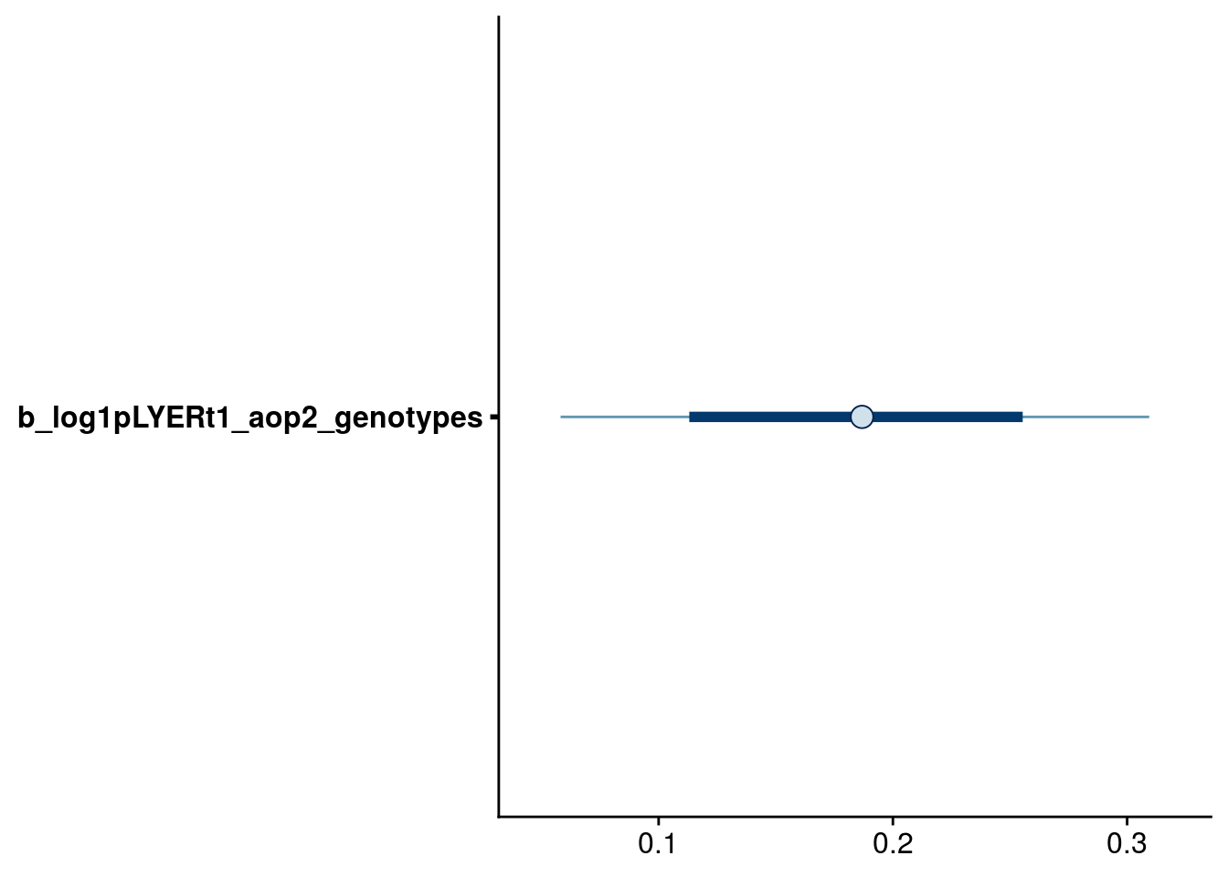
Check effect of AOP2\(-\).
pp_aop2_LP_persist(reduced.6.brm, temp.cond = 1.5, aop2.cond = 2)aop2_LPbound_BayesP aop2_LPbound_effect
0.996000 3.743655 The effect size is cut in half and the probability of this positive effect decreases slightly. In my mind, this indicates that it’s a bit worse than the 90% cutoff model in reproducing our observed data. Still, it also points to the fact that the effect of null AOP2\(-\) allele on LYER growth rates is the primary driver.
Structural stability of dominant food chain
Although we already identified which model is most approrpriate, now we are going to delve deeper into the specific effects.
aop2.brm <- reduced.5.brmReproduce Fig. 4
Since our observational data indicated clear effects of AOP2 gene on the persistence of the LYER-Ptoid subcommunity, I restrict our subsequent analysis to this effect (i.e. no temperature).
Note that I did not specify an effect of AOP2 on the intra- or interspecific interactions in LYER or Ptoid. Therefore, the interaction matrix is the same for both AOP2\(-\) and AOP2\(+\).
Also, I did this comparison at an imaginary midpoint of temperature, i.e. temp = 1.5. In this food chain, temperature only had a clear effect on the parasitoid’s intrinsic growth rate, so I only add the temperature effect here.
coef.aop2 <- fixef(aop2.brm)[,"Estimate"]

# value of rich to condition
temp.cond <- 1.5 # 1.5 = 21.5 C
# I chose 1.5 to condition on
# an imaginary average between temperature treatments
# note that setting it to zero, represents temp = 20 C

# interaction matrix for all levels of aop2
aop2.mat <- matrix(c(coef.aop2["log1pLYERt1_log1pLYER_t"],
                      coef.aop2["log1pLYERt1_log1pPtoid_t"],
                      coef.aop2["log1pPtoidt1_log1pLYER_t"],
                      0), # set to zero because there was no clear evidence for intraspecific Ptoid effect
                    ncol = 2, byrow = TRUE)
aop2.mat
[,1] [,2]
[1,] -0.6577923 -0.7203533
[2,] 0.3499795 0.0000000AOP2.mat <- aop2.mat
# growth rates with aop2 allele (both genotypes)
aop2.IGR <- matrix(c(coef.aop2["log1pLYERt1_intercept"] + coef.aop2["log1pLYERt1_aop2_genotypes"]*2,
coef.aop2["log1pPtoidt1_intercept"] + coef.aop2["log1pPtoidt1_aop2_genotypes"]*2 + coef.aop2["log1pPtoidt1_temp"]*temp.cond),
ncol = 1)
aop2.IGR [,1]
[1,] 3.852553
[2,] -1.665569# growth rates with AOP2 allele (both genotypes)
AOP2.IGR <- matrix(c(coef.aop2["log1pLYERt1_intercept"] + coef.aop2["log1pLYERt1_AOP2_genotypes"]*2,
coef.aop2["log1pPtoidt1_intercept"] + coef.aop2["log1pPtoidt1_AOP2_genotypes"]*2 + coef.aop2["log1pPtoidt1_temp"]*temp.cond),
ncol = 1)
AOP2.IGR [,1]
[1,] 3.319372
[2,] -2.048295Plot the effect of AOP2 gene on structural stability.
# get raw data for manually making plot
get_FD.2sp <- FeasibilityDomain2sp(A = list(aop2.mat, AOP2.mat),
                     r = list(aop2.IGR, AOP2.IGR),
                     labels = c("aop2", "AOP2"),
                     normalize = TRUE) %>%
  rename(aop2 = A_ID)

# Draw polygon for feasibility domain
# from: https://stackoverflow.com/questions/12794596/how-fill-part-of-a-circle-using-ggplot2
# define the circle; add a point at the center if the 'pie slice' if the shape is to be filled
circleFun <- function(center=c(0,0), diameter=1, npoints=100, start=0, end=2, filled=TRUE){
  tt <- seq(start*pi, end*pi, length.out=npoints)
  df <- data.frame(
    x = center[1] + diameter / 2 * cos(tt),
    y = center[2] + diameter / 2 * sin(tt)
  )
  if(filled==TRUE) { #add a point at the center so the whole 'pie slice' is filled
    df <- rbind(df, center)
  }
  return(df)
}

# new version
alpha_level <- 0.01
ggplot(filter(get_FD.2sp, Type == "r"), aes(x = Sp_1, y = Sp_2)) +
  # draw intrinsic growth rate vectors
  geom_segment(aes(x = 0, y = 0, xend = Sp_1, yend = Sp_2, color = aop2),
               arrow = arrow(type = 'open', length = unit(0.1,"cm"))) +
  # draw critical boundary (remove for final plot after adjusting geom_polygon)
  geom_segment(data = filter(get_FD.2sp, Type == "A")[1,], # just need one lower bound
               aes(x = 0, y = 0, xend = Sp_1, yend = Sp_2, linetype = "Critical\nboundary"),
               color = "black",
               size = 0.5) +
  xlab("Aphid growth rate (normalized)") +
  ylab("Parasitoid growth rate (normalized)") +
  # illustrate circular nature of feasibility domain
  coord_cartesian(xlim = c(0,1), ylim = c(0.0,-0.75), expand = F) +
  # make alpha very low for final plot to provide better looking arrows with keynote
  # scale_alpha_manual(values = c(alpha_level, alpha_level), labels = c("AOP2\u2013","AOP2+"), name = "") +
  # adjusted until critical boundary was correct, then removed critical boundary for final plot
  geom_polygon(data=circleFun(c(0,0), diameter = 2, start=0, end=-0.156, npoints=100, filled=TRUE),
               aes(x,y), alpha = 0.1, inherit.aes = F) +
  theme_cowplot(font_size = 18, line_size = 1)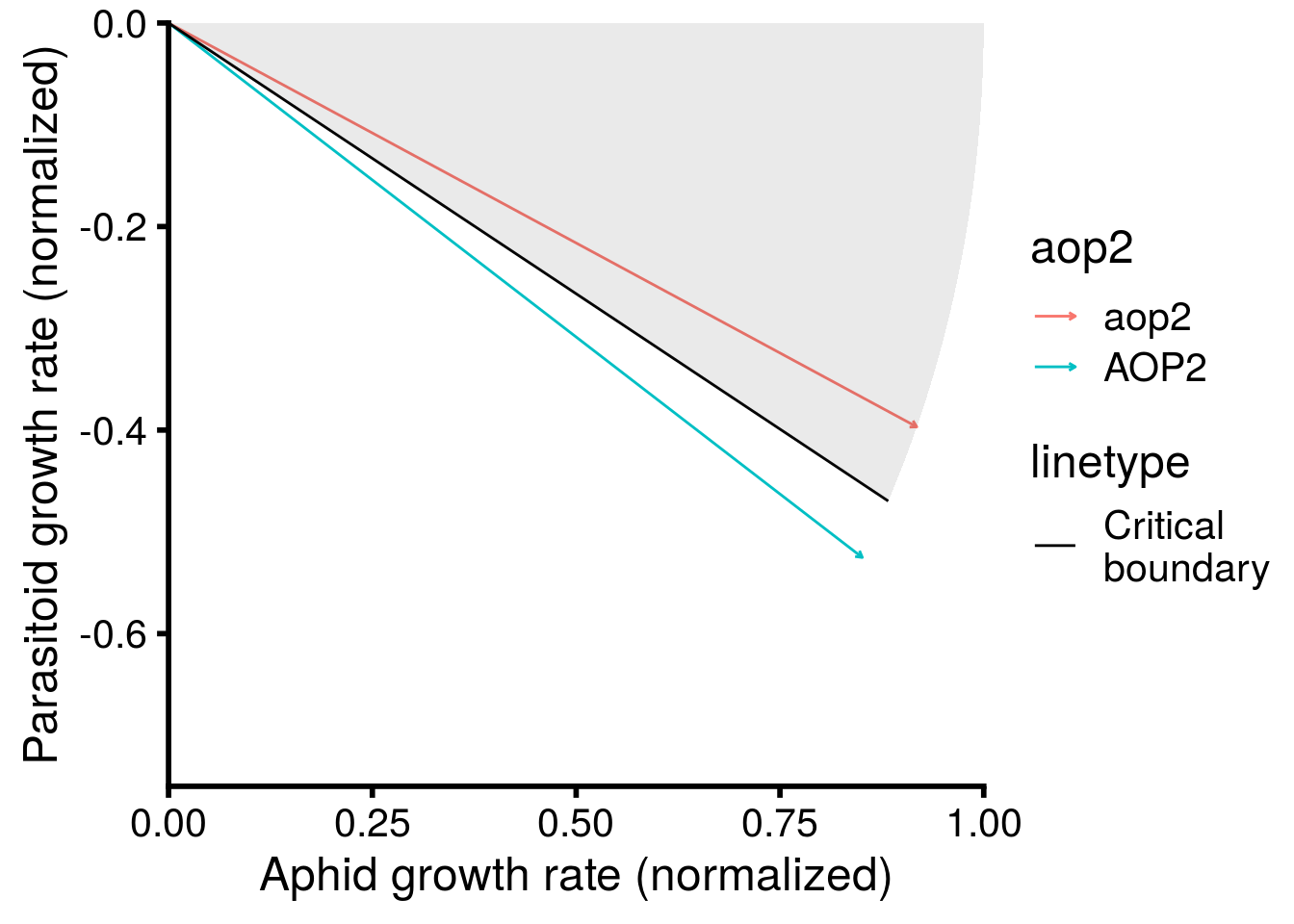
# changes for final version
# alpha = aop2 in geom_segment(aes())
# uncomment scale_alpha_manual
# remove dotted line for critical boundary
# ggsave("figures/keystone-structural-stability-forkeynote.pdf", width = 8, height = 8, units = "in")
I then used Keynote to manually add images and text to create the final version presented in Figure 4 of the main text.
And just as a quick check, the above plot suggests that the community is only feasible (all three species have positive abundances at equilibrium) when the plant population has both genotypes with AOP2\(-\) allele, which is true:
-inv(aop2.mat) %*% aop2.IGR [,1]
[1,] 4.759048
[2,] 1.002409-inv(AOP2.mat) %*% AOP2.IGR [,1]
[1,] 5.8526128
[2,] -0.7363496Non-equilibrium simulation (Fig. S5)
The above plot illustrates the effect of AOP2 on the structural stability of the equilibrium abundances of species. I can explore whether our results hold in a non-equilibrium scenario that better characterizes our observational data.
To do this, I look at the the effect of AOP2 across a range of initial conditions for the abundances of LYER and Ptoid. I get this data by simulating community dynamics with the observed effects of AOP2 across a range of initial conditions. I restricted our simulation to 10 time steps, as BRBR went extinct commonly at week 7 (experiment was 17 weeks long). I also set an extinction threshold of 2 individuals.
LP_duration <- 10
LP_threshold <- log(2) # set threshold of two individuals in the populations
res <- 0.1
LP_test_df <- expand.grid(LYER = seq(1, 6, by = res), Ptoid = seq(1, 6, by = res))

## simulate population dynamics and determine which species goes extinct

# aop2
FE_LP_aop2 <- list()
for(i in 1:length(LP_test_df$LYER)){
  FE_LP_aop2[[i]] <- first_extinction_2sp(Initial.States = c(LYER = LP_test_df[i,"LYER"], Ptoid = LP_test_df[i,"Ptoid"]),
                                          Interaction.Matrix = aop2.mat + diag(2),
                                          IGR.Vector = aop2.IGR,
                                          Duration = LP_duration,
                                          threshold = LP_threshold)
}
FE_LP_aop2_df <- bind_cols(LP_test_df, plyr::ldply(FE_LP_aop2)) %>%
  mutate(allele = "aop2")

# AOP2
FE_LP_AOP2 <- list()
for(i in 1:length(LP_test_df$LYER)){
  FE_LP_AOP2[[i]] <- first_extinction_2sp(Initial.States = c(LYER = LP_test_df[i,"LYER"], Ptoid = LP_test_df[i,"Ptoid"]),
                                           Interaction.Matrix = AOP2.mat + diag(2),
                                           IGR.Vector = AOP2.IGR,
                                           Duration = LP_duration,
                                           threshold = LP_threshold)
}
FE_LP_AOP2_df <- bind_cols(LP_test_df, plyr::ldply(FE_LP_AOP2)) %>%
  mutate(allele = "AOP2")

# get observed data on initial abundances of LYER and Ptoid after BRBR went extinct
LP_actual_df <- timeseries_df %>%
  filter(BRBR_t == 0, LYER_t > 0, Ptoid_t > 0) %>%
  group_by(Cage) %>% # rich,
  summarise_at(vars(LYER_t, Ptoid_t), list(first = first)) %>%
  ungroup() %>%
  mutate(#rich = rich + 1,
         log1p_LYER_t_first = log1p(LYER_t_first),
         log1p_Ptoid_t_first = log1p(Ptoid_t_first)) %>%
  as.data.frame()
The graph below shows a couple of useful things. First, our predictions hold for outside of equilibrium. That is, there is a greater likelihood of LYER-Ptoid persistence when there are genotypes with the null AOP2\(-\) allele in the population.
It’s also important to note that there is a region of parameter space where LYER goes extinct before Ptoid, which would eventually lead to the collapse of the Ptoid since it has lost its resource. This is not possible if I were to assume the community is at equilibrium.
cbPalette <-  viridis::viridis(4)

bind_rows(FE_LP_aop2_df, FE_LP_AOP2_df) %>%
  mutate(allele = factor(allele, labels = c("AOP2\u2013","AOP2+"))) %>%
  mutate(species = ifelse(is.na(species) == T, "Food chain persists", species),
         fspecies = factor(species, levels = c("LYER","Ptoid","Food chain persists"), labels = c("Complete collapse","Aphid only","Food chain persists"))) %>%
  ggplot(., aes(x = LYER, y = Ptoid, fill = fspecies)) + # fspecies
  geom_tile() +
  facet_grid(~allele) +
  scale_fill_manual(name = "Critical transition", values = cbPalette[1:3]) +
  coord_cartesian(xlim = c(1, max(LP_actual_df$log1p_LYER_t_first)),
                  ylim = c(1, max(LP_actual_df$log1p_Ptoid_t_first))) +
  xlab("Aphid initial abundance (log scale)") +
  ylab("Parasitoid initial abundance (log scale)") +
  theme_cowplot() +
theme(strip.background = element_blank()) 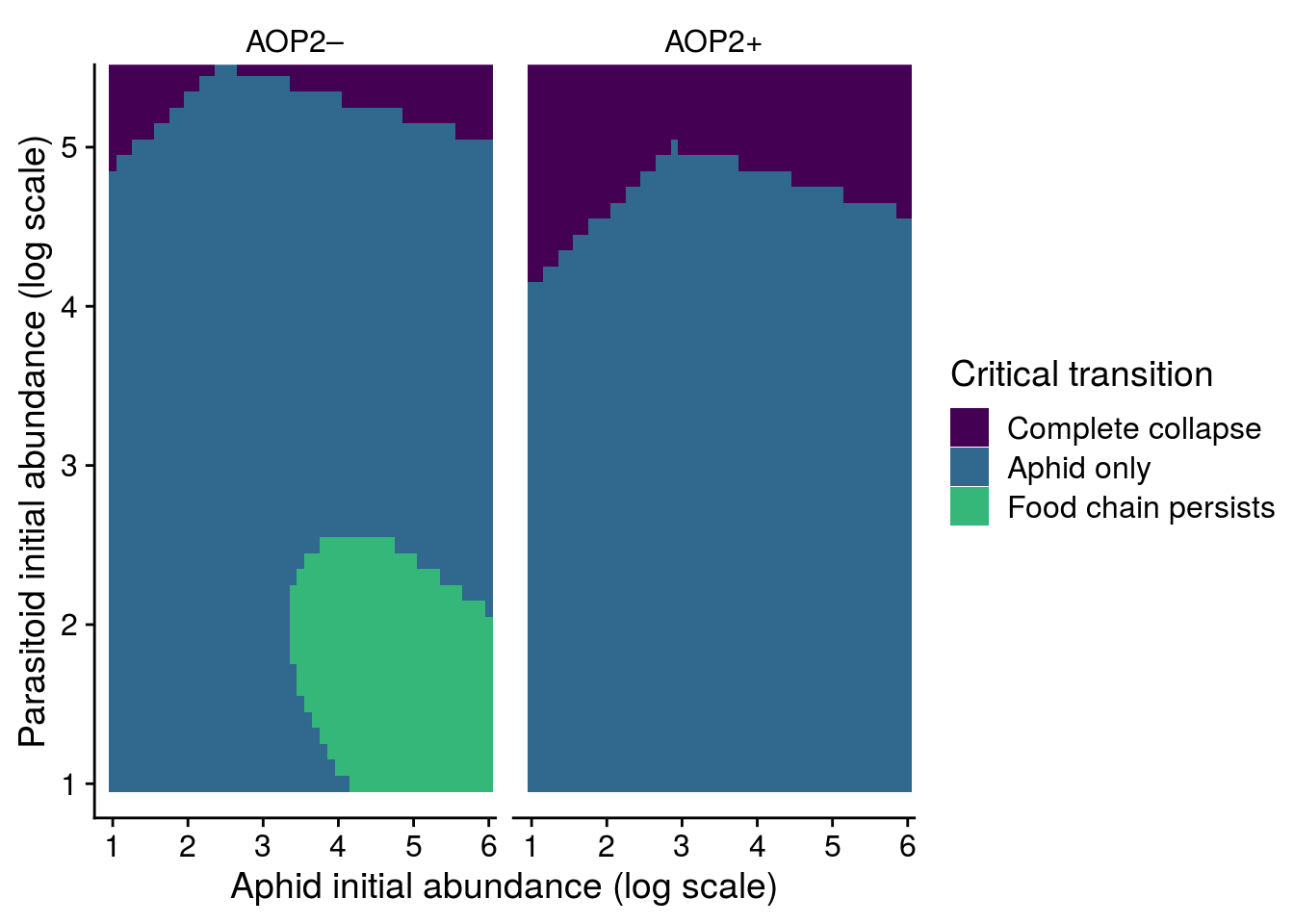
# ggsave(filename = "figures/MAR1-nonequilibrium-foodchain-AOP2.pdf", width = 6, height = 5, device=cairo_pdf)Remember though that our real communities are also stochastic, which is something I did not include in this non-equilibrium simulation. Below, I explicitly address stochasticity by estimating the uncertainty in our observed “mean” effects of AOP2 on structural stability.
Posterior estimates (Fig. S4)
The above is a nice visualization of the central tendency, but it doesn’t illustrate the uncertainty in the effect of AOP2 on structural stability. To get at this, I need to use the posterior samples from our model.
# note that this is virtually the same code in AOP2-LYER-Ptoid-persistence.R, but I detail
# it here for transparency and plotting.

# get posterior predictions
pp.aop2_model <- posterior_samples(aop2.brm, pars = "^b")

# calculate structural stability when aop2 = 2
aop2_stability <- apply(
  pp.aop2_model,
  MARGIN = 1,
  FUN = function(x) {
    tmp.mat = matrix(c(x["b_log1pLYERt1_log1pLYER_t"], x["b_log1pLYERt1_log1pPtoid_t"],
                       x["b_log1pPtoidt1_log1pLYER_t"], 0),
                     ncol = 2, byrow = TRUE)
    tmp.r = matrix(c(x["b_log1pLYERt1_intercept"] + x["b_log1pLYERt1_aop2_genotypes"]*2,
                     x["b_log1pPtoidt1_intercept"] + x["b_log1pPtoidt1_aop2_genotypes"]*2 + x["b_log1pPtoidt1_temp"]*temp.cond),
                   ncol = 1)
    FeasibilityBoundaryLYER.Ptoid = as.numeric(BoundaryLYER.Ptoid(tmp.mat, tmp.r)["boundary"])
    c(FeasibilityBoundaryLYER.Ptoid = FeasibilityBoundaryLYER.Ptoid)
  })
aop2_stability.df <- data.frame(
  allele = "aop2",
  posterior_sample = 1:nrow(pp.aop2_model),
  FeasibilityBoundaryLYER.Ptoid = aop2_stability
)

# calculate structural stability when rich = 2
AOP2_stability <- apply(
  pp.aop2_model,
  MARGIN = 1,
  FUN = function(x) {
    tmp.mat = matrix(c(x["b_log1pLYERt1_log1pLYER_t"], x["b_log1pLYERt1_log1pPtoid_t"],
                       x["b_log1pPtoidt1_log1pLYER_t"], 0),
                     ncol = 2, byrow = TRUE)
    tmp.r = matrix(c(x["b_log1pLYERt1_intercept"] + x["b_log1pLYERt1_AOP2_genotypes"]*2,
                     x["b_log1pPtoidt1_intercept"] + x["b_log1pPtoidt1_AOP2_genotypes"]*2 + x["b_log1pPtoidt1_temp"]*temp.cond),
                   ncol = 1)
    FeasibilityBoundaryLYER.Ptoid = as.numeric(BoundaryLYER.Ptoid(tmp.mat, tmp.r)["boundary"])
    c(FeasibilityBoundaryLYER.Ptoid = FeasibilityBoundaryLYER.Ptoid)
  })
AOP2_stability.df <- data.frame(
  allele = "AOP2",
  posterior_sample = 1:nrow(pp.aop2_model),
  FeasibilityBoundaryLYER.Ptoid = AOP2_stability
)

# combine data
all.aop2_stability.df <- bind_rows(aop2_stability.df, AOP2_stability.df)
Reproduce Fig. S4
# subsample 1/8 of the posterior to make it easier to visualize
set.seed(38)
rsamp <- sample(1:8000, size = 1000)

# plot
all.aop2_stability.df %>%
  filter(posterior_sample %in% rsamp) %>%
  mutate(n.allele = as.numeric(as.factor(allele))) %>%
  ggplot(., aes(x = n.allele, y = FeasibilityBoundaryLYER.Ptoid)) +
  geom_line(aes(group = posterior_sample), alpha = 0.1) +
  stat_summary(fun.y = mean, geom = "line", color = "firebrick1", size = 1) +
  stat_summary(fun.y = mean, geom = "point", color = "firebrick1", size = 1.5) +
  theme_minimal_hgrid() +
  scale_x_continuous(name = "Allele", breaks = c(1,2), labels = c("AOP2\u2013", "AOP2+"), expand = c(0.1,0.1)) +
ylab("Normalized angle from critical boundary") 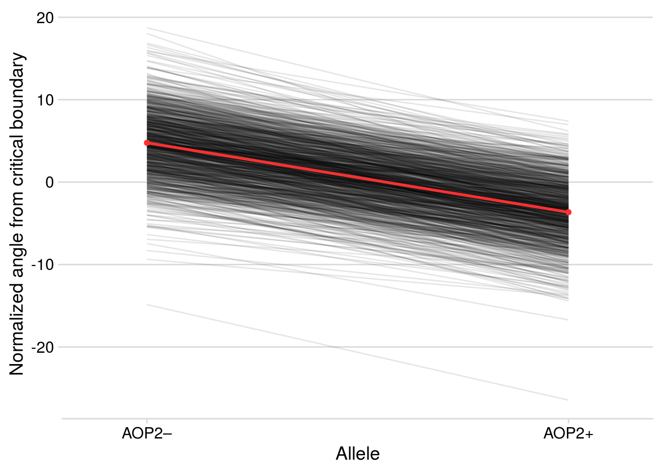
# ggsave(filename = "figures/MAR1-posterior-foodchain-AOP2.pdf", width = 6, height = 5, device=cairo_pdf)Calculate the percentage of posterior estimates where genetic diversity increased the structural stability of the community.
# organize data
aop2_LPbound <- all.aop2_stability.df %>%
  select(allele, posterior_sample, FeasibilityBoundaryLYER.Ptoid) %>%
  spread(allele, FeasibilityBoundaryLYER.Ptoid) %>%
  mutate(allele_effect = `aop2` - `AOP2`)

# calculate percentage
mean(aop2_LPbound$allele_effect > 0)
[1] 0.9995# calculate effect size
mean(aop2_LPbound$allele_effect)[1] 8.399152# note that this was all done in
pp_aop2_LP_persist(aop2.brm)aop2_LPbound_BayesP aop2_LPbound_effect
0.999500 8.399152 # but I broke it down to facilitate transparency and for plottingLet’s look at the effect of AOP2\(-\) on LYER and Ptoid’s intrinsic growth rates.
mean(pp.aop2_model$b_log1pLYERt1_aop2_genotypes)[1] 0.1882475mean(pp.aop2_model$b_log1pLYERt1_aop2_genotypes > 0)[1] 0.992875mean(pp.aop2_model$b_log1pPtoidt1_aop2_genotypes)[1] 0.1101749mean(pp.aop2_model$b_log1pPtoidt1_aop2_genotypes > 0)[1] 0.95825Structural stability of initial food web
I use the same model as I did for the effect of AOP2 aop2.brm.
temp_model <- aop2.brmReproduce Fig. S1
coef.temp <- fixef(temp_model)[,"Estimate"]

# we don't include AOP2 gene value, so it estimates at zero
# for both AOP2_genotypes and aop2_genotypes, i.e., an imaginary
# allele that reflects the intercept.
temp.cond <- 3

# interaction matrix when temp = 20 C
temp20.mat <- matrix(c(0,
                       0,
                       coef.temp["log1pBRBRt1_log1pPtoid_t"],
                       coef.temp["log1pLYERt1_log1pBRBR_t"],
                       coef.temp["log1pLYERt1_log1pLYER_t"],
                       coef.temp["log1pLYERt1_log1pPtoid_t"],
                       coef.temp["log1pPtoidt1_log1pBRBR_t"],
                       coef.temp["log1pPtoidt1_log1pLYER_t"],
                       0),
                     ncol = 3, byrow = TRUE)

# growth rates when temp = 20 C
temp20.IGR <- matrix(c(coef.temp["log1pBRBRt1_intercept"],
                       coef.temp["log1pLYERt1_intercept"],
                       coef.temp["log1pPtoidt1_intercept"]),
                     ncol = 1)

# interaction matrix when temp = 23 C
temp23.mat <- matrix(c(0,
                       0,
                       coef.temp["log1pBRBRt1_log1pPtoid_t"] + coef.temp["log1pBRBRt1_log1pPtoid_t:temp"]*temp.cond,
                       coef.temp["log1pLYERt1_log1pBRBR_t"],
                       coef.temp["log1pLYERt1_log1pLYER_t"],
                       coef.temp["log1pLYERt1_log1pPtoid_t"],
                       0,# constrained to biologically reasonable value of zero, rather than negative estimate # coef.temp["log1pPtoidt1_log1pBRBR_t"] + coef.temp["log1pPtoidt1_log1pBRBR_t:temp"]*3,
                       coef.temp["log1pPtoidt1_log1pLYER_t"],
                       0),
                     ncol = 3, byrow = TRUE)

# growth rates when temp = 23 C
temp23.IGR <- matrix(c(0.1, # constrained to biological reasonable value of 0.1, rather than negative estimate # coef.temp["log1pBRBRt1_intercept"] + coef.temp["log1pBRBRt1_temp"]*temp.cond,
                       coef.temp["log1pLYERt1_intercept"],
                       coef.temp["log1pPtoidt1_intercept"] + coef.temp["log1pPtoidt1_temp"]*temp.cond),
                     ncol = 1)

# assess feasibility
-1*inv(temp20.mat) %*% temp20.IGR # all species persist
[,1]
[1,] 3.684269
[2,] 4.544427
[3,] 1.827313-1*inv(temp23.mat) %*% temp23.IGR # BRBR goes extinct [,1]
[1,] -7.2344347
[2,] 2.5306054
[3,] 0.2534261# plot structural stability
constraints.matrix <- matrix(c(-1,0,0,
0,-1,0,
0,0,1),
ncol = 3, byrow = T)
PlotFeasibilityDomain3sp(A = list(temp20.mat, temp23.mat, constraints.matrix),
r = list(temp20.IGR, temp23.IGR, temp23.IGR), # IGR doesn't matter for constraints
A.color = c("steelblue","firebrick1","grey"),
r.color = c("steelblue","firebrick1","grey"),
normalize = TRUE,
sphere.alpha = 0,
arc.width = c(2,2,2),
barb.n = 2,
species.labels = c("B","L","P"))
# add axes
rgl.lines(x = c(0,1.1), y = c(0,0), z = c(0,0), color = "black", lwd = 3)
rgl.lines(x = c(0,0), y = c(1.1,0), z = c(0,0), color = "black", lwd = 3)
rgl.lines(x = c(0,0), y = c(0,0), z = c(-1.1,0), color = "black", lwd = 3)
# visualize in .html file
# note that I reproduce this visualization in `code/temperature-structural-stability-fig.R`
scene3d()RGL scene containing:
material: default material properties
objects: list of 40 object(s):
surface text text text linestrip linestrip linestrip linestrip linestrip linestrip linestrip points text text text linestrip linestrip linestrip linestrip linestrip linestrip linestrip points text text text linestrip linestrip linestrip linestrip linestrip linestrip linestrip points lines lines lines light background background
root: a root subscenerglwidget()From the above figure, it appears that the L-P boundary determines the feasibility of the community (alpha.A23 below). Therefore, I focus on estimating the normalized angle of the intrinsic growth rate from this critical boundary.
# calculate angle from critical boundary L-P for 23 C community
FeasibilityBoundary(temp23.mat, temp23.IGR)["alpha.A23"]
alpha.A23
-9.314478 Posterior estimates
# get posterior predictions
pp.temp_model <- posterior_samples(temp_model, pars = "^b")
Inspect parameter estimates to ensure they are biologically reasonable.
# most BRBR intrinsic growth rates are predicted to become negative with warming,
# which is not biological realistic. I will constrain these to a small positive value of 0.1
pp.temp_model %>%
  mutate(pp_ID = 1:nrow(.),
         r_BRBR_20 = b_log1pBRBRt1_intercept,
         r_BRBR_23 = b_log1pBRBRt1_intercept + b_log1pBRBRt1_temp*3) %>%
  select(pp_ID, r_BRBR_20, r_BRBR_23) %>%
  gather(key = temp, value = r, -pp_ID) %>%
  filter(pp_ID %in% rsamp) %>% # subsample to avoid crowding plot
  ggplot(., aes(x = temp, y = r)) +
  geom_line(aes(group = pp_ID), alpha = 0.1) +
  stat_summary(fun.y = mean, geom = "point", col = "red", size = 2) +
geom_hline(yintercept = 0, linetype = "dotted", color = "red") 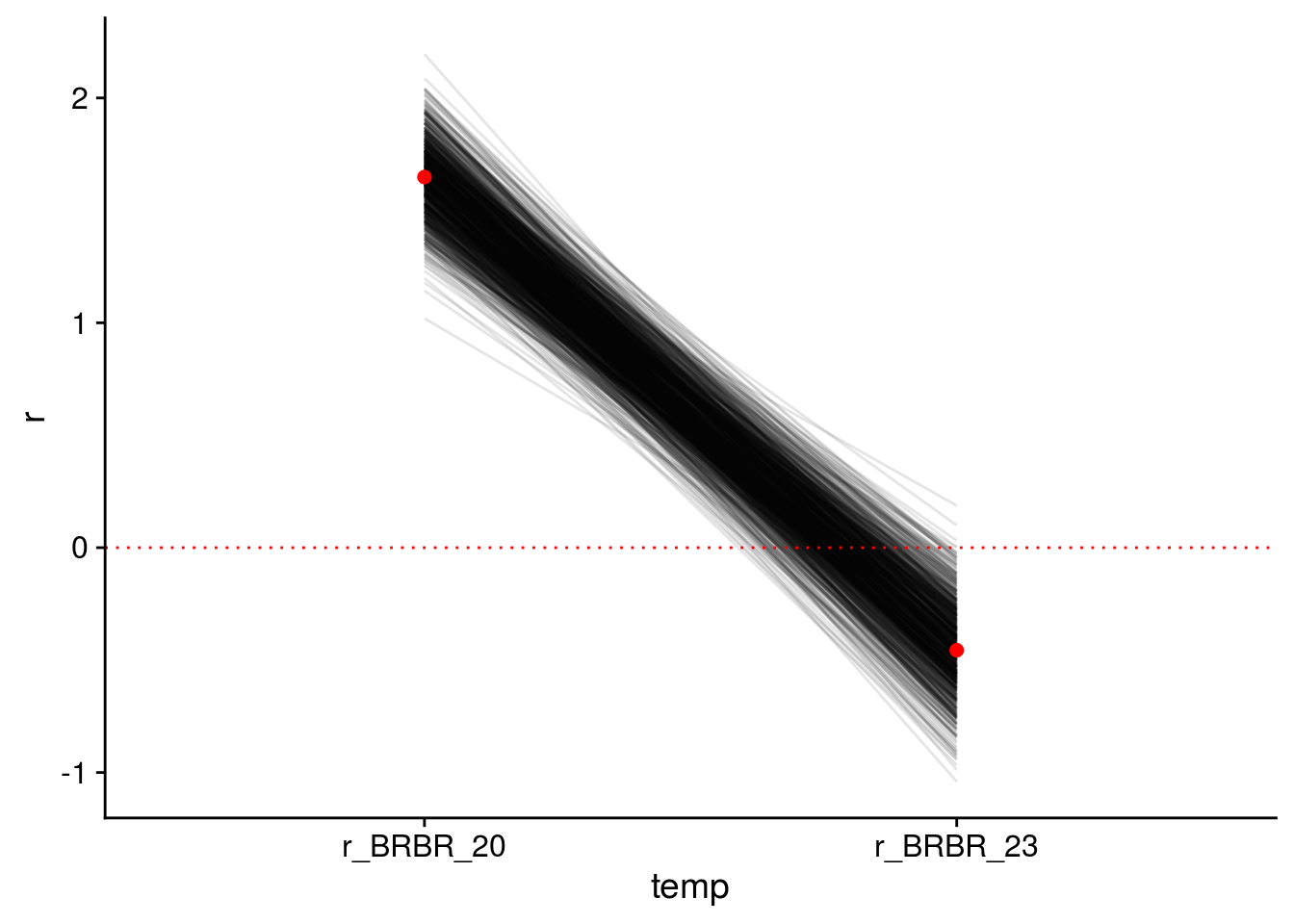
# the effect of BRBR on the parasitoid at warmer temperatures apparently
# becomes negative quite frequnetly. Rather than setting it to zero, I used a more conservative
# approach, by constraining the lower bound to zero, allowing positive effects
# in the posterior samples.
pp.temp_model %>%
  mutate(pp_ID = 1:nrow(.),
         BRBR_Ptoid_20 = b_log1pPtoidt1_log1pBRBR_t,
         BRBR_Ptoid_23 = b_log1pPtoidt1_log1pBRBR_t + `b_log1pPtoidt1_log1pBRBR_t:temp`*3) %>%
  select(pp_ID, BRBR_Ptoid_20, BRBR_Ptoid_23) %>%
  gather(key = temp, value = inter, -pp_ID) %>%
  filter(pp_ID %in% rsamp) %>% # subsample to avoid crowding plot
  ggplot(., aes(x = temp, y = inter)) +
  geom_line(aes(group = pp_ID), alpha = 0.1) +
  stat_summary(fun.y = mean, geom = "point", col = "red", size = 2) +
  geom_hline(yintercept = 0, linetype = "dotted", color = "red")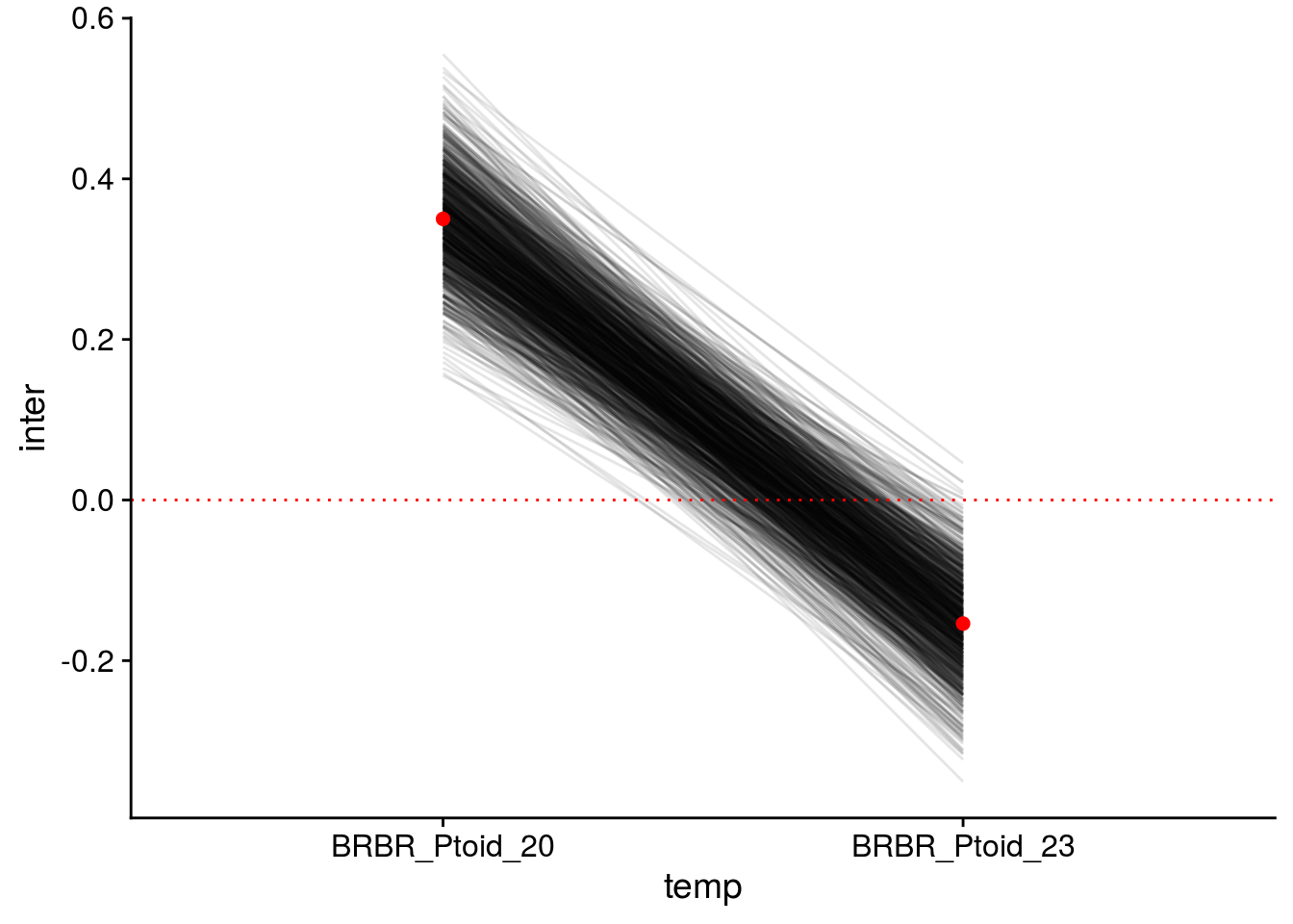
# rarely is the parasitoid's intrinsic growth rate estimated as positive,
# althought it should be negative
pp.temp_model %>%
  mutate(pp_ID = 1:nrow(.),
         r_BRBR_20 = b_log1pPtoidt1_intercept,
         r_BRBR_23 = b_log1pPtoidt1_intercept + b_log1pPtoidt1_temp*3) %>%
  select(pp_ID, r_BRBR_20, r_BRBR_23) %>%
  gather(key = temp, value = r, -pp_ID) %>%
  # use all samples to see occasional unrealistic estimate # filter(pp_ID %in% rsamp) %>% # subsample to avoid crowding plot
  ggplot(., aes(x = temp, y = r)) +
  geom_line(aes(group = pp_ID), alpha = 0.1) +
  stat_summary(fun.y = mean, geom = "point", col = "red", size = 2) +
geom_hline(yintercept = 0, linetype = "dotted", color = "red") 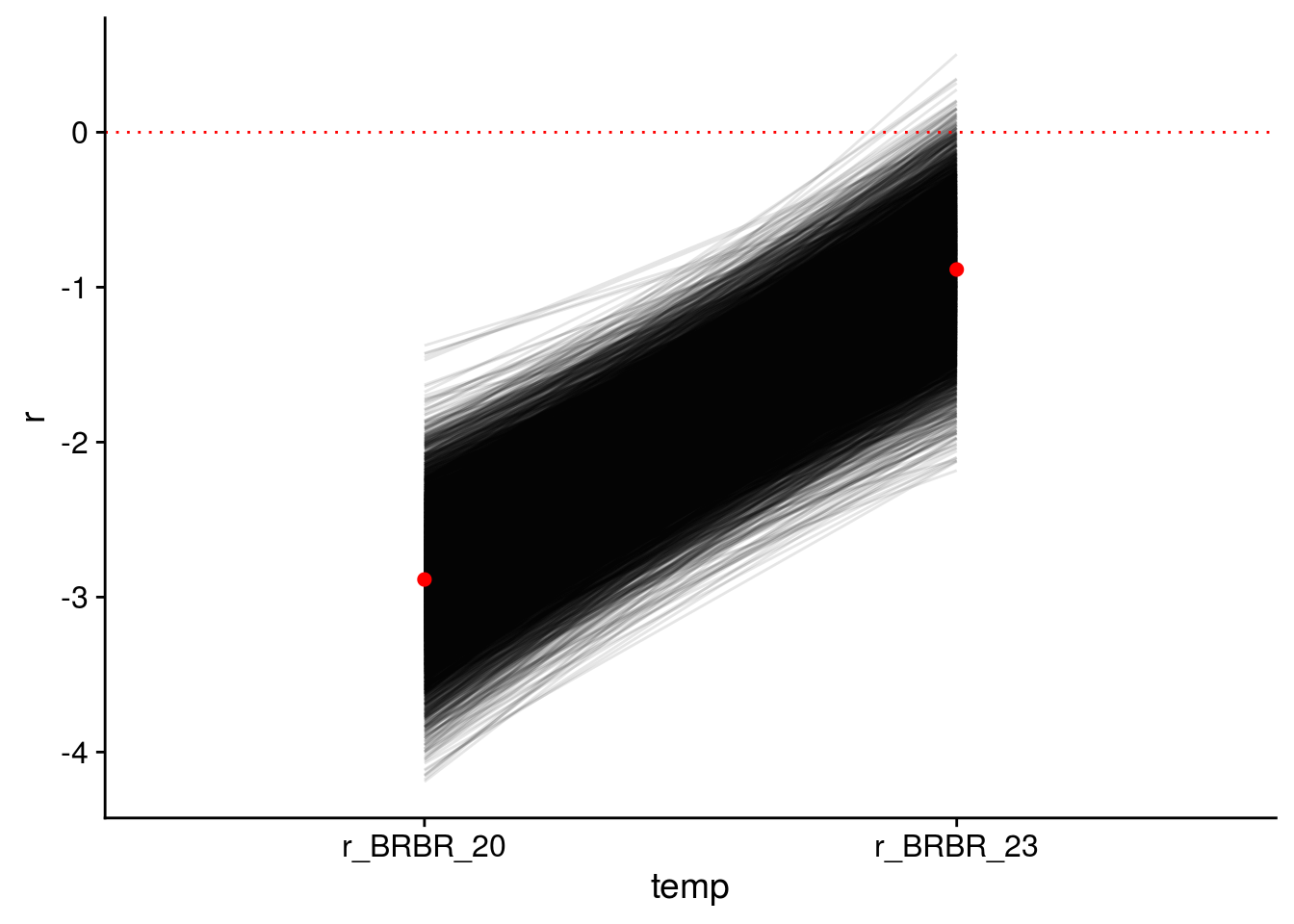
Note that some of the posterior samples can be biologically unfeasible, such as aphids with negative intrinsic growth rates. I restrict our inference to those parameters that are feasible. For example, if an aphid’s intrinsic growth rate was estimated as negative, I manually set it to a small positive value of 0.1. In terms of the interactions, I ensured that any apparent negative effects of aphids on the parasitoids was unrealistic, so I constrained this parameter to be zero or positive.
Note that if I went ahead without this biological restriction, our results remain qualitatively the same.
# get posterior samples of structural stability
temp20C_stability <- apply(
  pp.temp_model,
  MARGIN = 1,
  FUN = function(x) {
    tmp.mat = matrix(c(0,
                       0,
                       x["b_log1pBRBRt1_log1pPtoid_t"],
                       x["b_log1pLYERt1_log1pBRBR_t"],
                       x["b_log1pLYERt1_log1pLYER_t"],
                       x["b_log1pLYERt1_log1pPtoid_t"],
                       x["b_log1pPtoidt1_log1pBRBR_t"],
                       x["b_log1pPtoidt1_log1pLYER_t"],
                       0),
                     ncol = 3, byrow = TRUE)
    # constrain BRBR-Ptoid interaction to a min of zero
    if(tmp.mat[3,1] < 0){
       tmp.mat[3,1] <- 0
    }

    tmp.r = matrix(c(x["b_log1pBRBRt1_intercept"],
                     x["b_log1pLYERt1_intercept"],
                     x["b_log1pPtoidt1_intercept"]),
                   ncol = 1)
    # constrain BRBR intrinsic growth rate to positive values
    if(tmp.r[1] < 0){
      tmp.r[1] <- 0.1 # small positive value
    }
    # constrain Ptoid intrinsic growth rate to negative values
    if(tmp.r[3] > 0){
      tmp.r[3] <- -0.1 # small negative value
    }

    Feasibility = as.numeric(FeasibilityBoundary(tmp.mat, tmp.r)["feasibility"])
    FeasibilityBoundary23 = as.numeric(FeasibilityBoundary(tmp.mat, tmp.r)["alpha.A23"])
    Extinctions = paste0(which(-1*inv(tmp.mat) %*% tmp.r < 0), collapse = ",")
    Resilience = max(Re(eigen((tmp.mat + diag(3)))$values))
    list(tmp.mat = tmp.mat,
         tmp.r = tmp.r,
         Feasibility = Feasibility,
         FeasibilityBoundary23 = FeasibilityBoundary23,
         Extinctions = Extinctions,
         Resilience = Resilience)
  })
temp20C_stability.df <- data.frame(
  temp = "20 C",
  posterior_sample = 1:nrow(pp.temp_model),
  Feasibility = unlist(lapply(temp20C_stability, FUN = function(x) x$Feasibility)),
  FeasibilityBoundary23 = unlist(lapply(temp20C_stability, FUN = function(x) x$FeasibilityBoundary23)),
  Extinctions = unlist(lapply(temp20C_stability, FUN = function(x) x$Extinctions)),
  Resilience = unlist(lapply(temp20C_stability, FUN = function(x) x$Resilience))
)

temp23C_stability <- apply(
  pp.temp_model,
  MARGIN = 1,
  FUN = function(x) {
    tmp.mat = matrix(c(0,#x["b_log1pBRBRt1_log1pBRBR_t"] + x["b_log1pBRBRt1_log1pBRBR_t:temp"]*3,
                       0,
                       x["b_log1pBRBRt1_log1pPtoid_t"] + x["b_log1pBRBRt1_log1pPtoid_t:temp"]*3,
                       x["b_log1pLYERt1_log1pBRBR_t"],
                       x["b_log1pLYERt1_log1pLYER_t"],
                       x["b_log1pLYERt1_log1pPtoid_t"],
                       x["b_log1pPtoidt1_log1pBRBR_t"] + x["b_log1pPtoidt1_log1pBRBR_t:temp"]*3,
                       x["b_log1pPtoidt1_log1pLYER_t"],
                       0),
                     ncol = 3, byrow = TRUE)
    # constrain BRBR-Ptoid interaction to a min of zero
    if(tmp.mat[3,1] < 0){
       tmp.mat[3,1] <- 0
    }

    tmp.r = matrix(c(x["b_log1pBRBRt1_intercept"] + x["b_log1pBRBRt1_temp"]*3,
                     x["b_log1pLYERt1_intercept"],
                     x["b_log1pPtoidt1_intercept"] + x["b_log1pPtoidt1_temp"]*3),
                   ncol = 1)
    # constrain BRBR intrinsic growth rate to positive values
    if(tmp.r[1] < 0){
      tmp.r[1] <- 0.1 # small positive value
    }
    # constrain Ptoid intrinsic growth rate to negative values
    if(tmp.r[3] > 0){
      tmp.r[3] <- -0.1 # small negative value
    }

    Feasibility = as.numeric(FeasibilityBoundary(tmp.mat, tmp.r)["feasibility"])
    FeasibilityBoundary23 = as.numeric(FeasibilityBoundary(tmp.mat, tmp.r)["alpha.A23"])
    Extinctions = paste0(which(-1*inv(tmp.mat) %*% tmp.r < 0), collapse = ",")
    Resilience = max(Re(eigen((tmp.mat + diag(3)))$values))
    list(tmp.mat = tmp.mat,
         tmp.r = tmp.r,
         Feasibility = Feasibility,
         FeasibilityBoundary23 = FeasibilityBoundary23,
         Extinctions = Extinctions,
         Resilience = Resilience)
  })
temp23C_stability.df <- data.frame(
  temp = "23 C",
  posterior_sample = 1:nrow(pp.temp_model),
  Feasibility = unlist(lapply(temp23C_stability, FUN = function(x) x$Feasibility)),
  FeasibilityBoundary23 = unlist(lapply(temp23C_stability, FUN = function(x) x$FeasibilityBoundary23)),
  Extinctions = unlist(lapply(temp23C_stability, FUN = function(x) x$Extinctions)),
  Resilience = unlist(lapply(temp23C_stability, FUN = function(x) x$Resilience))
)


all.temp_stability.df <- bind_rows(temp20C_stability.df, temp23C_stability.df)
Reproduce Fig. S2
# Boundary determined by LYER-Ptoid (23)
all.temp_stability.df %>%
  filter(posterior_sample %in% rsamp) %>% # plot subset of posterior for easier visualization
  mutate(n.temp = as.numeric(as.factor(temp))) %>%
  ggplot(., aes(x = n.temp, y = FeasibilityBoundary23)) +
  geom_line(aes(group = posterior_sample), alpha = 0.1) +
  geom_hline(yintercept = 0, linetype = "dotted") +
  stat_summary(fun.y = mean, geom = "line", color = "red", size = 1) +
  stat_summary(fun.y = mean, geom = "point", color = "red", size = 1.5) +
  theme_minimal_hgrid() +
  scale_x_continuous(name = "Temperature", breaks = c(1,2), labels = c("20 C", "23 C"), expand = c(0.1,0.1)) +
  ylab("Normalized angle from critical boundary")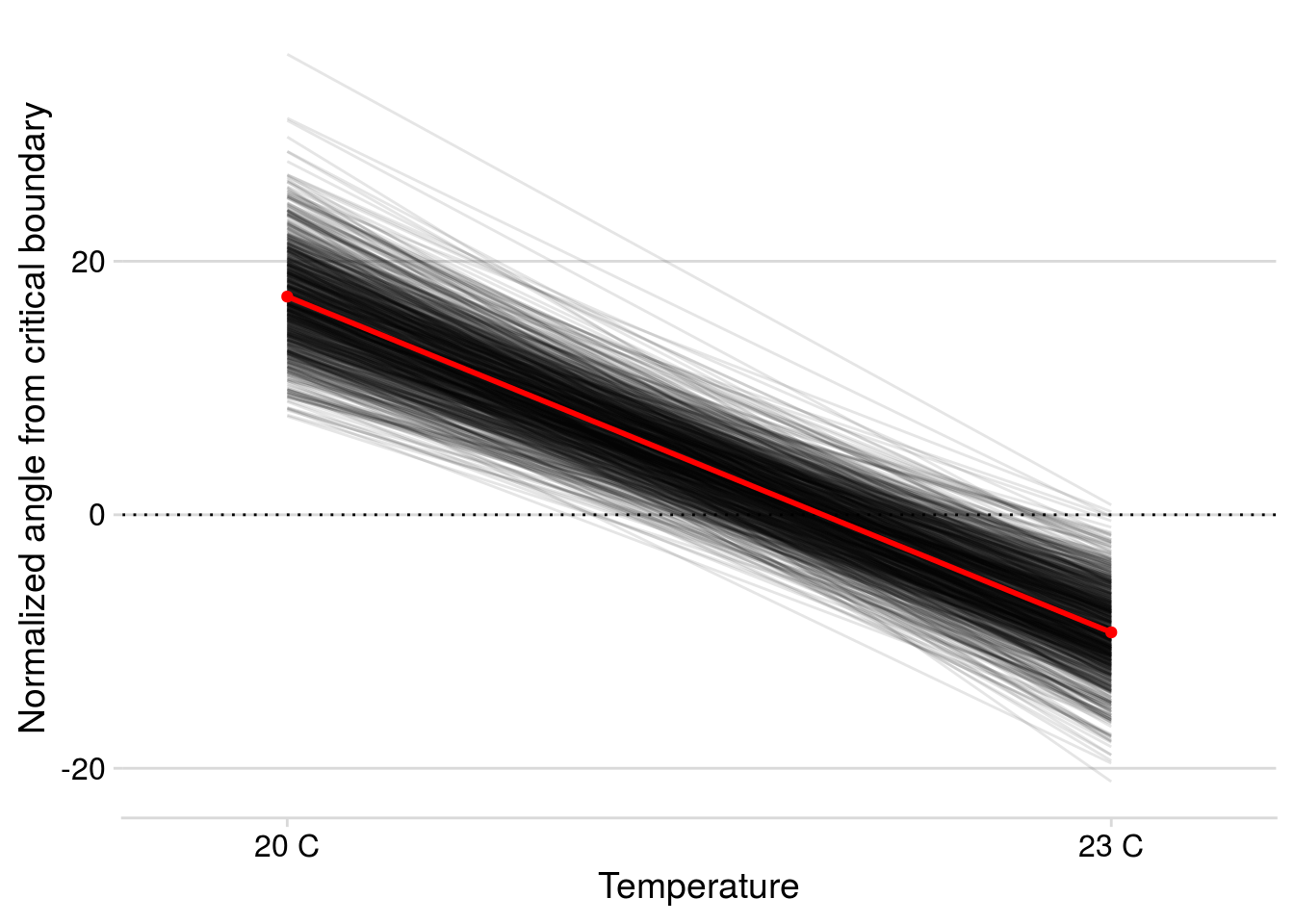
# ggsave(filename = "figures/MAR1-posterior-initial-temp.pdf", height = 5, width = 6)

## calculate percentage of posterior estimates where temperature decreases structural stability
# organize data
FeasibilityBoundary23_df <- all.temp_stability.df %>%
  select(temp, posterior_sample, FeasibilityBoundary23) %>%
  spread(key = temp, value = FeasibilityBoundary23) %>%
  mutate(Diff = `23 C` - `20 C`)
# calculate percentage
mean(FeasibilityBoundary23_df$Diff < 0)
[1] 1Non-equilibrium simulation (Fig. S3)
noneq_temp20 <- SimulateCommunityDynamics(IGR.Vector = temp20.IGR, Interaction.Matrix = (temp20.mat + diag(3)), Duration = 9) %>% mutate(temp = "20 C")

noneq_temp23 <- SimulateCommunityDynamics(IGR.Vector = temp23.IGR, Interaction.Matrix = (temp23.mat + diag(3)), Duration = 7) %>% mutate(temp = "23 C")

bind_rows(noneq_temp20, noneq_temp23) %>%
  gather(Species, value = "Abundance", -Week, - temp) %>%
  ggplot(., aes(x = Week, y = Abundance, color = Species)) +
  geom_hline(yintercept = 0, linetype = "dotted") +
  geom_line() +
  geom_point() +
  facet_wrap(~temp, ncol = 1) +
  theme_minimal_hgrid() +
  ylab("Abundance (log scale)") +
  scale_color_viridis_d(labels = c("B. brassicae","L. erysimi","D. rapae"))
# ggsave(filename = "figures/MAR1-nonequilibrium-initial-temp.pdf", height = 5, width = 6)Save analysis
Write out an .RData file to use for the Supplementary Online Materiak.
save.image(file = "output/structural-stability-keystone.RData")
sessionInfo()R version 3.6.3 (2020-02-29)
Platform: x86_64-pc-linux-gnu (64-bit)
Running under: Ubuntu 16.04.7 LTS
Matrix products: default
BLAS: /usr/lib/libblas/libblas.so.3.6.0
LAPACK: /usr/lib/lapack/liblapack.so.3.6.0
locale:
[1] LC_CTYPE=en_US.UTF-8 LC_NUMERIC=C
[3] LC_TIME=en_US.UTF-8 LC_COLLATE=en_US.UTF-8
[5] LC_MONETARY=en_US.UTF-8 LC_MESSAGES=en_US.UTF-8
[7] LC_PAPER=en_US.UTF-8 LC_NAME=C
[9] LC_ADDRESS=C LC_TELEPHONE=C
[11] LC_MEASUREMENT=en_US.UTF-8 LC_IDENTIFICATION=C
attached base packages:
[1] stats graphics grDevices utils datasets methods base
other attached packages:
[1] rgl_0.100.54 knitr_1.26 tidybayes_2.0.1 matlib_0.9.2
[5] cowplot_1.0.0 forcats_0.4.0 stringr_1.4.0 dplyr_0.8.3
[9] purrr_0.3.3 readr_1.3.1 tidyr_1.0.2 tibble_2.1.3
[13] ggplot2_3.2.1 tidyverse_1.3.0 brms_2.12.7 Rcpp_1.0.2
[17] RCurl_1.95-4.12 bitops_1.0-6
loaded via a namespace (and not attached):
[1] colorspace_1.4-1 ellipsis_0.3.0 rio_0.5.16
[4] ggridges_0.5.1 rsconnect_0.8.13 rprojroot_1.3-2
[7] markdown_1.1 base64enc_0.1-3 fs_1.3.1
[10] rstudioapi_0.10 rstan_2.19.2 svUnit_0.7-12
[13] DT_0.6 fansi_0.4.0 mvtnorm_1.0-10
[16] lubridate_1.7.4 xml2_1.2.2 bridgesampling_0.6-0
[19] shinythemes_1.1.2 bayesplot_1.7.0 jsonlite_1.6
[22] workflowr_1.6.0 broom_0.5.2 dbplyr_1.4.2
[25] broom.mixed_0.2.6 shiny_1.3.2 compiler_3.6.3
[28] httr_1.4.1 backports_1.1.4 assertthat_0.2.1
[31] Matrix_1.2-17 lazyeval_0.2.2 cli_1.1.0
[34] later_1.0.0 htmltools_0.3.6 prettyunits_1.0.2
[37] tools_3.6.3 igraph_1.2.4.1 coda_0.19-2
[40] gtable_0.3.0 glue_1.3.1 reshape2_1.4.3
[43] carData_3.0-2 cellranger_1.1.0 vctrs_0.2.2
[46] nlme_3.1-140 crosstalk_1.0.0 xfun_0.9
[49] ps_1.3.0 openxlsx_4.1.0.1 rvest_0.3.5
[52] mime_0.7 miniUI_0.1.1.1 lifecycle_0.1.0
[55] gtools_3.8.1 MASS_7.3-51.4 zoo_1.8-6
[58] scales_1.0.0 colourpicker_1.0 hms_0.5.3
[61] promises_1.0.1 Brobdingnag_1.2-6 parallel_3.6.3
[64] inline_0.3.15 TMB_1.7.18 shinystan_2.5.0
[67] curl_4.0 yaml_2.2.0 gridExtra_2.3
[70] loo_2.2.0 StanHeaders_2.19.0 stringi_1.4.3
[73] dygraphs_1.1.1.6 zip_2.0.3 pkgbuild_1.0.3
[76] manipulateWidget_0.10.0 rlang_0.4.4 pkgconfig_2.0.2
[79] matrixStats_0.54.0 evaluate_0.14 lattice_0.20-38
[82] labeling_0.3 rstantools_2.0.0 htmlwidgets_1.3
[85] processx_3.3.1 tidyselect_0.2.5 plyr_1.8.4
[88] magrittr_1.5 R6_2.4.0 generics_0.0.2
[91] DBI_1.0.0 foreign_0.8-71 pillar_1.4.2
[94] haven_2.2.0 whisker_0.3-2 withr_2.1.2
[97] xts_0.11-2 abind_1.4-5 car_3.0-3
[100] modelr_0.1.5 crayon_1.3.4 arrayhelpers_1.1-0
[103] utf8_1.1.4 rmarkdown_2.0 viridis_0.5.1
[106] grid_3.6.3 readxl_1.3.1 data.table_1.12.2
[109] callr_3.2.0 git2r_0.26.1 threejs_0.3.1
[112] reprex_0.3.0 digest_0.6.20 webshot_0.5.1
[115] xtable_1.8-4 httpuv_1.5.1 stats4_3.6.3
[118] munsell_0.5.0 viridisLite_0.3.0 shinyjs_1.0