Bayesian MAR(1) models and structural stability

workflowr

• Summary
• Checks
• Past versions

Last updated: 2020-06-23

Checks: 7 0

Knit directory: genes-to-foodweb-stability/

This reproducible R Markdown analysis was created with workflowr (version 1.6.0). The Checks tab describes the reproducibility checks that were applied when the results were created. The Past versions tab lists the development history.

---

R Markdown file: up-to-date

Great! Since the R Markdown file has been committed to the Git repository, you know the exact version of the code that produced these results.

Environment: empty

Great job! The global environment was empty. Objects defined in the global environment can affect the analysis in your R Markdown file in unknown ways. For reproduciblity it’s best to always run the code in an empty environment.

Seed: set.seed(20200205)

The command set.seed(20200205) was run prior to running the code in the R Markdown file. Setting a seed ensures that any results that rely on randomness, e.g. subsampling or permutations, are reproducible.

Session information: recorded

Great job! Recording the operating system, R version, and package versions is critical for reproducibility.

Cache: none

Nice! There were no cached chunks for this analysis, so you can be confident that you successfully produced the results during this run.

File paths: relative

Great job! Using relative paths to the files within your workflowr project makes it easier to run your code on other machines.

Repository version: 4088702

Great! You are using Git for version control. Tracking code development and connecting the code version to the results is critical for reproducibility. The version displayed above was the version of the Git repository at the time these results were generated.

Note that you need to be careful to ensure that all relevant files for the analysis have been committed to Git prior to generating the results (you can use wflow_publish or wflow_git_commit). workflowr only checks the R Markdown file, but you know if there are other scripts or data files that it depends on. Below is the status of the Git repository when the results were generated:

Ignored files:
    Ignored:    .Rhistory
    Ignored:    .Rproj.user/
    Ignored:    code/.Rhistory

Untracked files:
    Untracked:  figures/rich-geno-critical-transition.pdf

Unstaged changes:
    Modified:   figures/rich-geno-critical-transition-v4.pdf
    Modified:   output/critical-transitions.RData

Note that any generated files, e.g. HTML, png, CSS, etc., are not included in this status report because it is ok for generated content to have uncommitted changes.

---

These are the previous versions of the R Markdown and HTML files. If you’ve configured a remote Git repository (see ?wflow_git_remote), click on the hyperlinks in the table below to view them.

File	Version	Author	Date	Message
Rmd	86116c8	mabarbour	2020-06-23	bioRxiv version of code and data.
html	86116c8	mabarbour	2020-06-23	bioRxiv version of code and data.

---

Setup

# load data
timeseries_df <- read_csv("output/timeseries_df.csv") %>%
  mutate(# this makes the intercept correspond to rich = 1, rather
         # than the biologically implausible rich = 0
         rich = rich - 1,
         # now rich and temp coefficients will correspond to +1 genotype and +1 C
         temp = ifelse(temp == "20 C", 0, 3),
         uniq = paste(Cage, temp, com, Week_match, sep = "-"),
         Week_match.1p = 1 + Week_match) # analysis doesn't like initial Week_match = 0, so I just added 1

# filter dataset for multivariate analysis.
# I only retain data for which all species had positive abundances at the previous time step
full_df <- filter(timeseries_df, BRBR_t > 0, LYER_t > 0, Ptoid_t > 0) 

## source in useful functions

# functions for plotting feasibility domains and calculating normalized angles from critical boundary
source("code/plot-feasibility-domain.R") 
# functions for non-equilibrium simulation
source("code/simulate-community-dynamics.R")

Full model

This model corresponds to equation 1 in the Supplementary Material of the paper. Note that BRBR = aphid Brevicoryne brassicae, LYER = aphid Lipaphis erysimi, and Ptoid = parasitoid Diaeretiella rapae.

# BRBR
full.mv.norm.BRBR.bf <- bf(log1p(BRBR_t1) ~ 
                       0 + intercept + offset(log1p(BRBR_t)) + 
                        (log1p(BRBR_t) + log1p(LYER_t) + log1p(Ptoid_t))*(temp + rich) +
                        log(Biomass_g_t1) +
                        (1 | Cage) +
                        ar(time = Week_match.1p, gr = Cage, p = 1, cov = FALSE))

# LYER
full.mv.norm.LYER.bf <- bf(log1p(LYER_t1) ~ 
                       0 + intercept + offset(log1p(LYER_t)) + 
                        (log1p(BRBR_t) + log1p(LYER_t) + log1p(Ptoid_t))*(temp + rich) +
                        log(Biomass_g_t1) +
                        (1 | Cage) +
                        ar(time = Week_match.1p, gr = Cage, p = 1, cov = FALSE))

# Ptoid
full.mv.norm.Ptoid.bf <- bf(log1p(Ptoid_t1) ~ 
                       0 + intercept + offset(log1p(Ptoid_t)) + 
                        (log1p(BRBR_t) + log1p(LYER_t) + log1p(Ptoid_t))*(temp + rich) +
                        log(Biomass_g_t1) +
                        (1 | Cage) +
                        ar(time = Week_match.1p, gr = Cage, p = 1, cov = FALSE))

Set priors

Intrinsic growth rates

# from Jahan et al. 2014, Journal of Insect Science
# Table 4 lambda (finite rate of increase, discrete time analogue of intrinsic growth rate)
# calculated on a per-day basis and not logged. This is why I multiply by 7 and then take the natural logarithm
Jahan.r.BRBR <- log(c(1.42, 1.36, 1.32, 1.35, 1.40, 1.33, 1.38, 1.37) * 7)
mean(Jahan.r.BRBR) # 2.26

[1] 2.257713

sd(Jahan.r.BRBR) # 0.02

[1] 0.02468356

# visualize prior
hist(rnorm(1000, mean(Jahan.r.BRBR), sd = 1))

Past versions of r-priors-1.png

Version	Author	Date
86116c8	mabarbour	2020-06-23

prior.r.BRBR <- "normal(2.26, 1)"

# from Taghizadeh 2019, J. Agr. Sci. Tech.
# Table 2 lambda (finite rate of increase, discrete time analogue of intrinsic growth rate)
# calculated on a per-day basis and not logged. This is why I multiply by 7 and then take the natural logarithm
Tag.r.LYER <- log(c(1.35, 1.30, 1.26, 1.23) * 7)
mean(Tag.r.LYER) # 2.20

[1] 2.196059

sd(Tag.r.LYER) # 0.04

[1] 0.04028153

# visualize prior
hist(rnorm(1000, mean(Tag.r.LYER), sd = 1))

Past versions of r-priors-2.png

Version	Author	Date
86116c8	mabarbour	2020-06-23

prior.r.LYER <- "normal(2.20, 1)"

# random effects prior based on variance among cultivars
# I'm just going to use this for all of them
mean.r.sd <- mean(c(sd(Jahan.r.BRBR), sd(Tag.r.LYER)))
# visualize prior
hist(rnorm(1000, mean = mean.r.sd, sd = 0.5))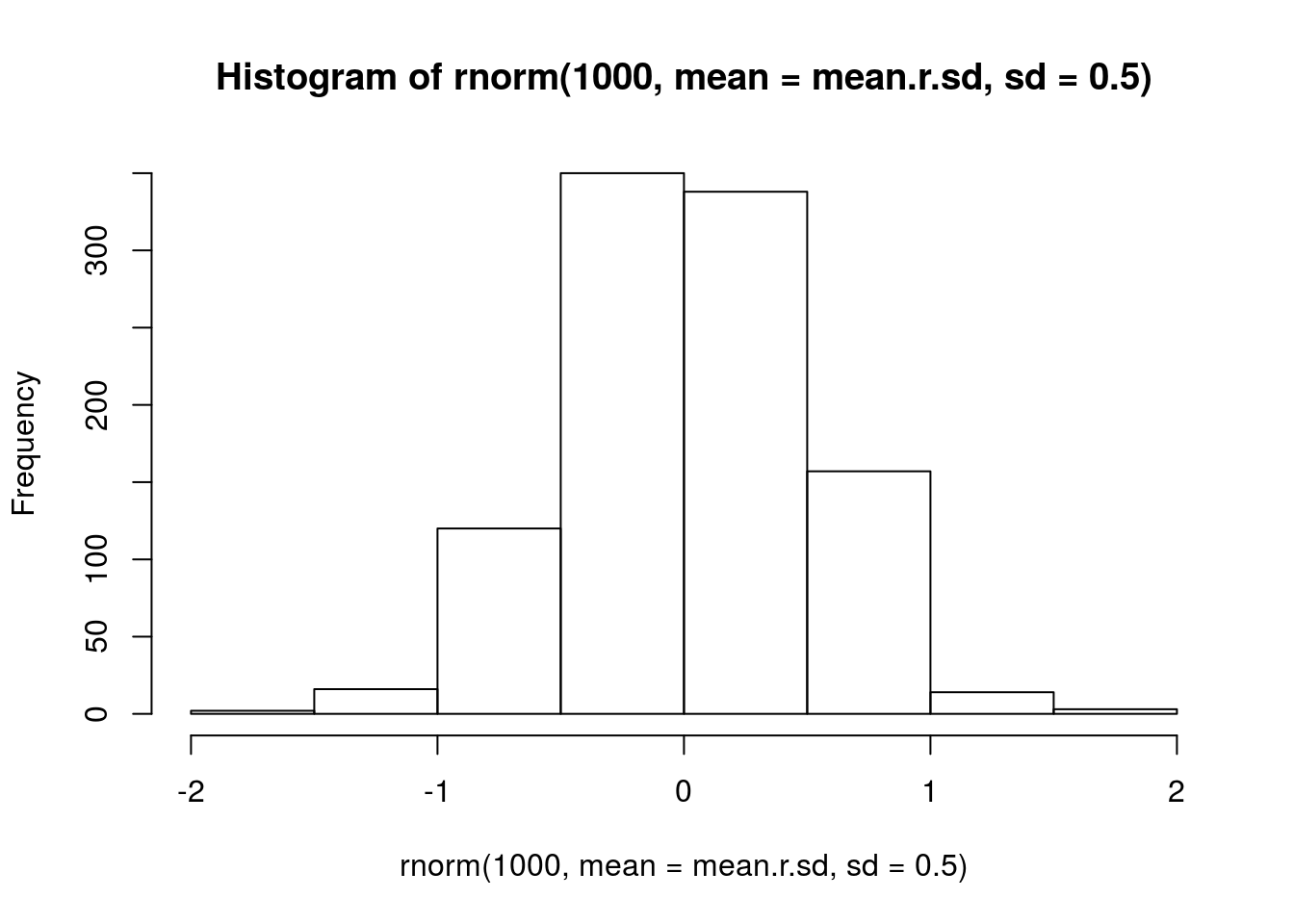

Past versions of r-priors-3.png

Version	Author	Date
86116c8	mabarbour	2020-06-23

prior.random.effects <- "normal(0.03, 0.5)"

# I don't have a great sense for the growth rate of the parasitoid, other than that it should be negative
# this seems like a reasonable starting point

# visualize prior
hist(rnorm(1000, mean = -1.5, sd = 1))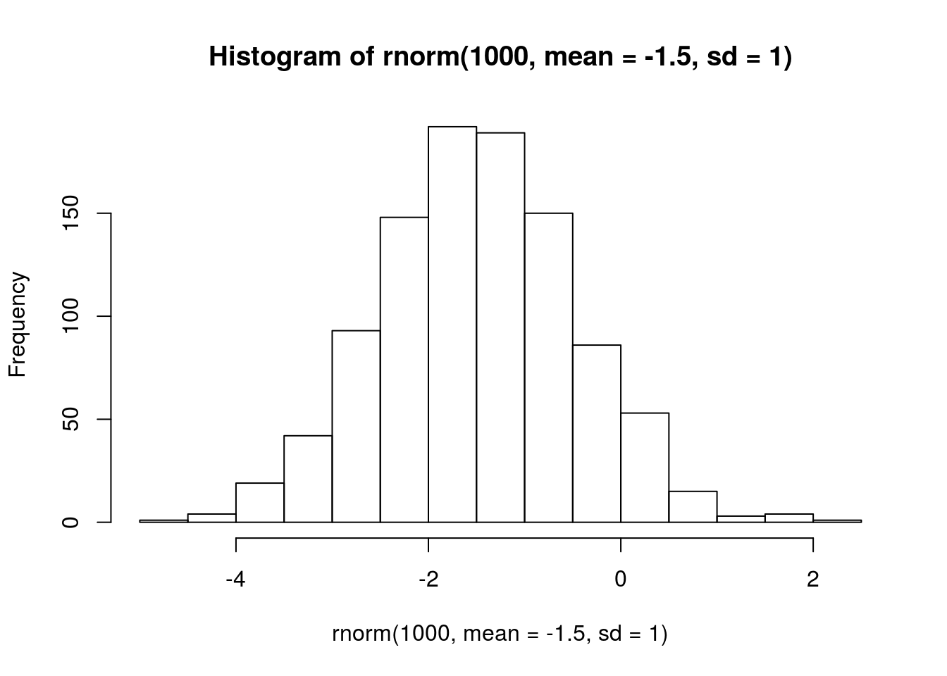

Past versions of r-priors-4.png

Version	Author	Date
86116c8	mabarbour	2020-06-23

prior.r.Ptoid <- "normal(-1.5, 1)"

Intra- and interspecific interactions

I assume they are weak, i.e. much less than \(|1|\). I also assume that all species exhibit intraspecific competition, aphids have negative interspecific effects with each other, but positive interspecific effects on the parasitoid. I also assume parasitoids have negative interspecific effects on the aphids.

## intraspecific, 0 = no density dependence. this occurs because of offset in model.
# visualize prior
hist(rnorm(1000, mean = -0.1, sd = 0.5))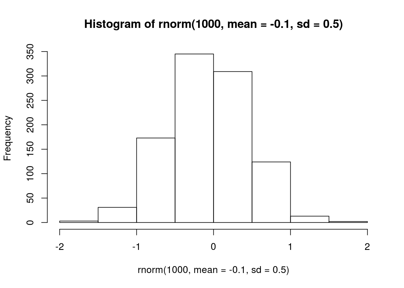

Past versions of interaction-priors-1.png

Version	Author	Date
86116c8	mabarbour	2020-06-23

prior.intra.BRBR <- "normal(-0.1, 0.5)"
prior.intra.LYER <- "normal(-0.1, 0.5)"
prior.intra.Ptoid <- "normal(-0.1, 0.5)"

## negative interspecific, 0 = no interaction
# visualize prior
hist(rnorm(1000, mean = -0.1, sd = 0.5))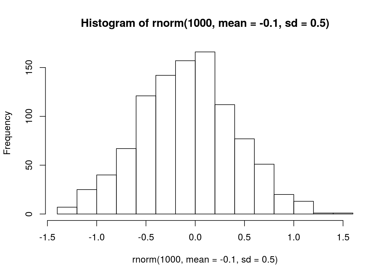

Past versions of interaction-priors-2.png

Version	Author	Date
86116c8	mabarbour	2020-06-23

# most of these values are less than 1, which
# is indicative of saturating effects
prior.LYERonBRBR <- "normal(-0.1, 0.5)" 
prior.PtoidonBRBR <- "normal(-0.1, 0.5)"
prior.BRBRonLYER <- "normal(-0.1, 0.5)"
prior.PtoidonLYER <- "normal(-0.1, 0.5)"

## positive interspecific
# visualize prior
hist(rnorm(1000, mean = 0.1, sd = 0.5))

Past versions of interaction-priors-3.png

Version	Author	Date
86116c8	mabarbour	2020-06-23

# most of these values are less than 1, which
# is indicative of saturating effects
prior.BRBRonPtoid <- "normal(0.1, 0.5)"
prior.LYERonPtoid <- "normal(0.1, 0.5)"

Genetic richness and genotype effects

It was unclear to me a priori exactly how genetic diversity and specific genotypes would affect species’ growth rates or intra- and interspecific interactions. Therefore, I assumed these effects on specific rates could be positive or negative, but would likely be between -1 and 1 (i.e., not ridiculously large).

prior.rich <- "normal(0, 0.5)"

I used prior.rich as the prior for genotype-specific effects as well.

Temperature effects

prior.temp <- "normal(0, 0.5)"

Biomass effects

For both aphids, I thought that increasing biomass would increase their intrinsic growth rates, but only weakly, because I didn’t expect biomass to be limiting.

# visualize prior
hist(rnorm(1000, mean = 0.1, sd = 0.5))

Past versions of aphid-biomass-priors-1.png

Version	Author	Date
86116c8	mabarbour	2020-06-23

prior.AphidBiomass <- "normal(0.1, 0.5)"

For the parasitoid, it was unclear to me whether increasing biomass would have positive or negative effects. I could imagine both, as increasing biomass may increase the search effort of parasitoids, resulting in a negative effect on their growth rate. Alternatively, more biomass may increase the quality of aphids, which could increase the parasitoid’s growth rate. Therefore, I specified a normal prior with mean = 0 and SD = 0.5, so that most of the distribution lied between -1 and 1 (i.e. saturating negative or positive effects).

# visualize prior
hist(rnorm(1000, mean = 0, sd = 0.5))

Past versions of ptoid-biomass-prior-1.png

Version	Author	Date
86116c8	mabarbour	2020-06-23

prior.PtoidBiomass <- "normal(0, 0.5)"

Analysis

I first fit a complete model with rich and temperature effects

full.mv.norm.brm <- brm(
  data = full_df,
  formula = mvbf(full.mv.norm.BRBR.bf, full.mv.norm.LYER.bf, full.mv.norm.Ptoid.bf),
  iter = 4000,
  prior = c(# growth rates
            set_prior(prior.r.BRBR, class = "b", coef = "intercept", resp = "log1pBRBRt1"),
            set_prior(prior.r.LYER, class = "b", coef = "intercept", resp = "log1pLYERt1"),
            set_prior(prior.r.Ptoid, class = "b", coef = "intercept", resp = "log1pPtoidt1"),
            # intraspecific effects
            set_prior(prior.intra.BRBR, class = "b", coef = "log1pBRBR_t", resp = "log1pBRBRt1"),
            set_prior(prior.intra.LYER, class = "b", coef = "log1pLYER_t", resp = "log1pLYERt1"),
            set_prior(prior.intra.LYER, class = "b", coef = "log1pPtoid_t", resp = "log1pPtoidt1"),
            # negative interspecific effects
            set_prior(prior.LYERonBRBR, class = "b", coef = "log1pLYER_t", resp = "log1pBRBRt1"),
            set_prior(prior.BRBRonLYER, class = "b", coef = "log1pBRBR_t", resp = "log1pLYERt1"),
            set_prior(prior.PtoidonBRBR, class = "b", coef = "log1pPtoid_t", resp = "log1pBRBRt1"),
            set_prior(prior.PtoidonLYER, class = "b", coef = "log1pPtoid_t", resp = "log1pLYERt1"),
            # positive interspecific effects
            set_prior(prior.BRBRonPtoid, class = "b", coef = "log1pBRBR_t", resp = "log1pPtoidt1"),
            set_prior(prior.LYERonPtoid, class = "b", coef = "log1pLYER_t", resp = "log1pPtoidt1"),
            # rich effects
            set_prior(prior.rich, class = "b", coef = "rich", resp = "log1pBRBRt1"),
            set_prior(prior.rich, class = "b", coef = "rich", resp = "log1pLYERt1"),
            set_prior(prior.rich, class = "b", coef = "rich", resp = "log1pPtoidt1"),  
            set_prior(prior.rich, class = "b", coef = "log1pBRBR_t:rich", resp = "log1pBRBRt1"),
            set_prior(prior.rich, class = "b", coef = "log1pBRBR_t:rich", resp = "log1pLYERt1"),
            set_prior(prior.rich, class = "b", coef = "log1pBRBR_t:rich", resp = "log1pPtoidt1"),
            set_prior(prior.rich, class = "b", coef = "log1pLYER_t:rich", resp = "log1pBRBRt1"),
            set_prior(prior.rich, class = "b", coef = "log1pLYER_t:rich", resp = "log1pLYERt1"),
            set_prior(prior.rich, class = "b", coef = "log1pLYER_t:rich", resp = "log1pPtoidt1"),
            set_prior(prior.rich, class = "b", coef = "log1pPtoid_t:rich", resp = "log1pBRBRt1"),
            set_prior(prior.rich, class = "b", coef = "log1pPtoid_t:rich", resp = "log1pLYERt1"),
            set_prior(prior.rich, class = "b", coef = "log1pPtoid_t:rich", resp = "log1pPtoidt1"),
            # temp effects
            set_prior(prior.temp, class = "b", coef = "temp", resp = "log1pBRBRt1"),
            set_prior(prior.temp, class = "b", coef = "temp", resp = "log1pLYERt1"),
            set_prior(prior.temp, class = "b", coef = "temp", resp = "log1pPtoidt1"),  
            set_prior(prior.temp, class = "b", coef = "log1pBRBR_t:temp", resp = "log1pBRBRt1"),
            set_prior(prior.temp, class = "b", coef = "log1pBRBR_t:temp", resp = "log1pLYERt1"),
            set_prior(prior.temp, class = "b", coef = "log1pBRBR_t:temp", resp = "log1pPtoidt1"),
            set_prior(prior.temp, class = "b", coef = "log1pLYER_t:temp", resp = "log1pBRBRt1"),
            set_prior(prior.temp, class = "b", coef = "log1pLYER_t:temp", resp = "log1pLYERt1"),
            set_prior(prior.temp, class = "b", coef = "log1pLYER_t:temp", resp = "log1pPtoidt1"),
            set_prior(prior.temp, class = "b", coef = "log1pPtoid_t:temp", resp = "log1pBRBRt1"),
            set_prior(prior.temp, class = "b", coef = "log1pPtoid_t:temp", resp = "log1pLYERt1"),
            set_prior(prior.temp, class = "b", coef = "log1pPtoid_t:temp", resp = "log1pPtoidt1"),
            # biomass effects
            set_prior(prior.AphidBiomass, class = "b", coef = "logBiomass_g_t1", resp = "log1pBRBRt1"),
            set_prior(prior.AphidBiomass, class = "b", coef = "logBiomass_g_t1", resp = "log1pLYERt1"),
            set_prior(prior.PtoidBiomass, class = "b", coef = "logBiomass_g_t1", resp = "log1pPtoidt1"),
            # random effects
            set_prior(prior.random.effects, class = "sd", resp = "log1pBRBRt1"),
            set_prior(prior.random.effects, class = "sd", resp = "log1pLYERt1"),
            set_prior(prior.random.effects, class = "sd", resp = "log1pPtoidt1")),
  file = "output/full.mv.norm.brm.rds") 

# print summary
summary(full.mv.norm.brm)

 Family: MV(gaussian, gaussian, gaussian) 
  Links: mu = identity; sigma = identity
         mu = identity; sigma = identity
         mu = identity; sigma = identity 
Formula: log1p(BRBR_t1) ~ 0 + intercept + offset(log1p(BRBR_t)) + (log1p(BRBR_t) + log1p(LYER_t) + log1p(Ptoid_t)) * (temp + rich) + log(Biomass_g_t1) + (1 | Cage) + ar(time = Week_match.1p, gr = Cage, p = 1, cov = FALSE) 
         log1p(LYER_t1) ~ 0 + intercept + offset(log1p(LYER_t)) + (log1p(BRBR_t) + log1p(LYER_t) + log1p(Ptoid_t)) * (temp + rich) + log(Biomass_g_t1) + (1 | Cage) + ar(time = Week_match.1p, gr = Cage, p = 1, cov = FALSE) 
         log1p(Ptoid_t1) ~ 0 + intercept + offset(log1p(Ptoid_t)) + (log1p(BRBR_t) + log1p(LYER_t) + log1p(Ptoid_t)) * (temp + rich) + log(Biomass_g_t1) + (1 | Cage) + ar(time = Week_match.1p, gr = Cage, p = 1, cov = FALSE) 
   Data: full_df (Number of observations: 264) 
Samples: 4 chains, each with iter = 4000; warmup = 2000; thin = 1;
         total post-warmup samples = 8000

Correlation Structures:
                   Estimate Est.Error l-95% CI u-95% CI Rhat Bulk_ESS Tail_ESS
ar_log1pBRBRt1[1]     -0.45      0.10    -0.63    -0.25 1.00     3525     5191
ar_log1pLYERt1[1]     -0.12      0.11    -0.32     0.10 1.00     7178     6071
ar_log1pPtoidt1[1]    -0.49      0.08    -0.65    -0.32 1.00    11047     6451

Group-Level Effects: 
~Cage (Number of levels: 60) 
                           Estimate Est.Error l-95% CI u-95% CI Rhat Bulk_ESS
sd(log1pBRBRt1_Intercept)      0.31      0.11     0.06     0.52 1.00      852
sd(log1pLYERt1_Intercept)      0.13      0.08     0.01     0.31 1.00     1928
sd(log1pPtoidt1_Intercept)     0.04      0.03     0.00     0.12 1.00     4679
                           Tail_ESS
sd(log1pBRBRt1_Intercept)      1308
sd(log1pLYERt1_Intercept)      3987
sd(log1pPtoidt1_Intercept)     3766

Population-Level Effects: 
                               Estimate Est.Error l-95% CI u-95% CI Rhat
log1pBRBRt1_intercept              1.39      0.63     0.17     2.63 1.00
log1pBRBRt1_log1pBRBR_t            0.04      0.13    -0.22     0.30 1.00
log1pBRBRt1_log1pLYER_t            0.03      0.15    -0.26     0.32 1.00
log1pBRBRt1_log1pPtoid_t          -0.93      0.07    -1.06    -0.79 1.00
log1pBRBRt1_temp                  -0.30      0.28    -0.87     0.25 1.00
log1pBRBRt1_rich                   0.03      0.35    -0.66     0.73 1.00
log1pBRBRt1_logBiomass_g_t1       -0.12      0.19    -0.49     0.26 1.00
log1pBRBRt1_log1pBRBR_t:temp      -0.08      0.05    -0.18     0.03 1.00
log1pBRBRt1_log1pBRBR_t:rich      -0.06      0.06    -0.18     0.06 1.00
log1pBRBRt1_log1pLYER_t:temp       0.00      0.06    -0.11     0.11 1.00
log1pBRBRt1_log1pLYER_t:rich       0.03      0.07    -0.10     0.16 1.00
log1pBRBRt1_log1pPtoid_t:temp      0.11      0.04     0.04     0.19 1.00
log1pBRBRt1_log1pPtoid_t:rich      0.04      0.05    -0.06     0.14 1.00
log1pLYERt1_intercept              2.73      0.62     1.52     3.99 1.00
log1pLYERt1_log1pBRBR_t            0.39      0.11     0.17     0.60 1.00
log1pLYERt1_log1pLYER_t           -0.67      0.14    -0.95    -0.40 1.00
log1pLYERt1_log1pPtoid_t          -0.70      0.07    -0.84    -0.57 1.00
log1pLYERt1_temp                   0.12      0.25    -0.37     0.62 1.00
log1pLYERt1_rich                   0.26      0.33    -0.39     0.90 1.00
log1pLYERt1_logBiomass_g_t1        0.27      0.17    -0.06     0.60 1.00
log1pLYERt1_log1pBRBR_t:temp      -0.04      0.05    -0.13     0.05 1.00
log1pLYERt1_log1pBRBR_t:rich      -0.12      0.05    -0.22    -0.01 1.00
log1pLYERt1_log1pLYER_t:temp       0.02      0.05    -0.08     0.12 1.00
log1pLYERt1_log1pLYER_t:rich       0.06      0.06    -0.06     0.17 1.00
log1pLYERt1_log1pPtoid_t:temp     -0.03      0.04    -0.10     0.04 1.00
log1pLYERt1_log1pPtoid_t:rich      0.01      0.04    -0.08     0.09 1.00
log1pPtoidt1_intercept            -2.81      0.49    -3.77    -1.84 1.00
log1pPtoidt1_log1pBRBR_t           0.47      0.08     0.31     0.63 1.00
log1pPtoidt1_log1pLYER_t           0.24      0.10     0.05     0.43 1.00
log1pPtoidt1_log1pPtoid_t         -0.04      0.05    -0.14     0.06 1.00
log1pPtoidt1_temp                  0.45      0.23     0.01     0.90 1.00
log1pPtoidt1_rich                 -0.13      0.31    -0.73     0.47 1.00
log1pPtoidt1_logBiomass_g_t1      -0.48      0.13    -0.73    -0.24 1.00
log1pPtoidt1_log1pBRBR_t:temp     -0.18      0.04    -0.25    -0.11 1.00
log1pPtoidt1_log1pBRBR_t:rich     -0.06      0.04    -0.13     0.01 1.00
log1pPtoidt1_log1pLYER_t:temp      0.05      0.04    -0.03     0.12 1.00
log1pPtoidt1_log1pLYER_t:rich      0.07      0.05    -0.02     0.17 1.00
log1pPtoidt1_log1pPtoid_t:temp     0.02      0.03    -0.04     0.08 1.00
log1pPtoidt1_log1pPtoid_t:rich     0.01      0.04    -0.06     0.08 1.00
                               Bulk_ESS Tail_ESS
log1pBRBRt1_intercept              8958     6192
log1pBRBRt1_log1pBRBR_t            4440     4605
log1pBRBRt1_log1pLYER_t            3941     4878
log1pBRBRt1_log1pPtoid_t           8029     5772
log1pBRBRt1_temp                   8151     5968
log1pBRBRt1_rich                   8200     6098
log1pBRBRt1_logBiomass_g_t1        9358     6174
log1pBRBRt1_log1pBRBR_t:temp       7094     6330
log1pBRBRt1_log1pBRBR_t:rich       7707     6285
log1pBRBRt1_log1pLYER_t:temp       6942     6010
log1pBRBRt1_log1pLYER_t:rich       6892     5878
log1pBRBRt1_log1pPtoid_t:temp      7172     6399
log1pBRBRt1_log1pPtoid_t:rich      8596     6372
log1pLYERt1_intercept              7495     6509
log1pLYERt1_log1pBRBR_t            6752     4912
log1pLYERt1_log1pLYER_t            5984     5991
log1pLYERt1_log1pPtoid_t           8024     6620
log1pLYERt1_temp                   8112     6310
log1pLYERt1_rich                   9047     6188
log1pLYERt1_logBiomass_g_t1       12846     5477
log1pLYERt1_log1pBRBR_t:temp       7169     5455
log1pLYERt1_log1pBRBR_t:rich       9261     5894
log1pLYERt1_log1pLYER_t:temp       6889     5984
log1pLYERt1_log1pLYER_t:rich       7706     6119
log1pLYERt1_log1pPtoid_t:temp      8851     6469
log1pLYERt1_log1pPtoid_t:rich      8328     6615
log1pPtoidt1_intercept             7110     6276
log1pPtoidt1_log1pBRBR_t           9065     5996
log1pPtoidt1_log1pLYER_t           7049     6085
log1pPtoidt1_log1pPtoid_t          8160     6448
log1pPtoidt1_temp                  8378     6562
log1pPtoidt1_rich                  7032     5692
log1pPtoidt1_logBiomass_g_t1      13747     6410
log1pPtoidt1_log1pBRBR_t:temp      9783     6497
log1pPtoidt1_log1pBRBR_t:rich     11800     5788
log1pPtoidt1_log1pLYER_t:temp      8403     6467
log1pPtoidt1_log1pLYER_t:rich      7642     6381
log1pPtoidt1_log1pPtoid_t:temp     9237     6362
log1pPtoidt1_log1pPtoid_t:rich     7580     6576

Family Specific Parameters: 
                   Estimate Est.Error l-95% CI u-95% CI Rhat Bulk_ESS Tail_ESS
sigma_log1pBRBRt1      1.10      0.06     0.99     1.23 1.00     2349     4577
sigma_log1pLYERt1      0.93      0.04     0.85     1.02 1.00     9800     6189
sigma_log1pPtoidt1     0.77      0.04     0.70     0.84 1.00    15372     5800

Residual Correlations: 
                                 Estimate Est.Error l-95% CI u-95% CI Rhat
rescor(log1pBRBRt1,log1pLYERt1)      0.52      0.05     0.42     0.62 1.00
rescor(log1pBRBRt1,log1pPtoidt1)    -0.04      0.07    -0.18     0.10 1.00
rescor(log1pLYERt1,log1pPtoidt1)     0.06      0.06    -0.06     0.19 1.00
                                 Bulk_ESS Tail_ESS
rescor(log1pBRBRt1,log1pLYERt1)      7359     5636
rescor(log1pBRBRt1,log1pPtoidt1)    10955     6627
rescor(log1pLYERt1,log1pPtoidt1)    13533     5975

Samples were drawn using sampling(NUTS). For each parameter, Bulk_ESS
and Tail_ESS are effective sample size measures, and Rhat is the potential
scale reduction factor on split chains (at convergence, Rhat = 1).

Inspect credible intervals

Below, I inspect which parameters may be safely omitted from the model. It seemed reasonable that if 80% of the posterior probability distribution of the parameter included zero, then I could safely drop it from the model. Therefore, I proceeded with this criteria, starting with the highest-order terms:

# higher-order temperature effects
bayesplot::mcmc_intervals(full.mv.norm.brm, regex_pars = "_t:temp$", prob = 0.80, prob_outer = 0.95) # drop LYER:temp effect on BRBR; all Species:temp effects on LYER; and (LYER and Ptoid):temp effects on Ptoid

Past versions of full-mv-norm-highest-order-1.png

Version	Author	Date
86116c8	mabarbour	2020-06-23

# higher-order rich effects
bayesplot::mcmc_intervals(full.mv.norm.brm, regex_pars = "_t:rich$", prob = 0.80, prob_outer = 0.95) # drop all Species:rich effect on BRBR; drop (LYER and Ptoid):rich effects on LYER; drop Ptoid:rich effect on Ptoid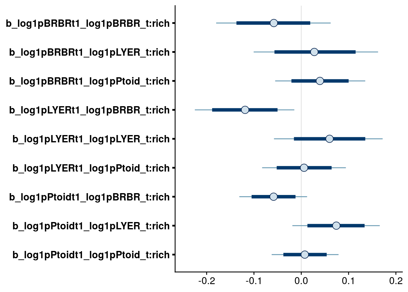

Past versions of full-mv-norm-highest-order-2.png

Version	Author	Date
86116c8	mabarbour	2020-06-23

Model selection

Reduced model 1

Drop terms

Based on the above plots, I dropped the following higher-order terms:

Effects on BRBR_t1:

• (log1p(LYER_t) + log1p(BRBR_t) + log1p(Ptoid_t)):rich
• log1p(LYER_t):temp

Effects on LYER_t1:

• (log1p(LYER_t) + log1p(BRBR_t) + log1p(Ptoid_t)):temp
• (log1p(LYER_t) + log1p(Ptoid_t)):rich

Effects on Ptoid_t1

• (log1p(LYER_t) + log1p(Ptoid_t)):temp
• log1p(Ptoid_t):rich

Refit model

# update formulas
reduced.1.BRBR.bf <- update(full.mv.norm.BRBR.bf, .~. -(log1p(LYER_t) + log1p(BRBR_t) + log1p(Ptoid_t)):rich -log1p(LYER_t):temp)
reduced.1.LYER.bf <- update(full.mv.norm.LYER.bf, .~. -(log1p(LYER_t) + log1p(BRBR_t) + log1p(Ptoid_t)):temp -(log1p(LYER_t) + log1p(Ptoid_t)):rich)
reduced.1.Ptoid.bf <- update(full.mv.norm.Ptoid.bf, .~. -(log1p(LYER_t) + log1p(Ptoid_t)):temp -log1p(Ptoid_t):rich)

# fit update model
reduced.1.brm <- brm(
  data = full_df,
  formula = mvbf(reduced.1.BRBR.bf, reduced.1.LYER.bf, reduced.1.Ptoid.bf),
  iter = 4000,
  prior = c(# growth rates
            set_prior(prior.r.BRBR, class = "b", coef = "intercept", resp = "log1pBRBRt1"),
            set_prior(prior.r.LYER, class = "b", coef = "intercept", resp = "log1pLYERt1"),
            set_prior(prior.r.Ptoid, class = "b", coef = "intercept", resp = "log1pPtoidt1"),
            # intraspecific effects
            set_prior(prior.intra.BRBR, class = "b", coef = "log1pBRBR_t", resp = "log1pBRBRt1"),
            set_prior(prior.intra.LYER, class = "b", coef = "log1pLYER_t", resp = "log1pLYERt1"),
            set_prior(prior.intra.LYER, class = "b", coef = "log1pPtoid_t", resp = "log1pPtoidt1"),
            # negative interspecific effects
            set_prior(prior.LYERonBRBR, class = "b", coef = "log1pLYER_t", resp = "log1pBRBRt1"),
            set_prior(prior.BRBRonLYER, class = "b", coef = "log1pBRBR_t", resp = "log1pLYERt1"),
            set_prior(prior.PtoidonBRBR, class = "b", coef = "log1pPtoid_t", resp = "log1pBRBRt1"),
            set_prior(prior.PtoidonLYER, class = "b", coef = "log1pPtoid_t", resp = "log1pLYERt1"),
            # positive interspecific effects
            set_prior(prior.BRBRonPtoid, class = "b", coef = "log1pBRBR_t", resp = "log1pPtoidt1"),
            set_prior(prior.LYERonPtoid, class = "b", coef = "log1pLYER_t", resp = "log1pPtoidt1"),
            # rich effects
            set_prior(prior.rich, class = "b", coef = "rich", resp = "log1pBRBRt1"),
            set_prior(prior.rich, class = "b", coef = "rich", resp = "log1pLYERt1"),
            set_prior(prior.rich, class = "b", coef = "rich", resp = "log1pPtoidt1"),  
            set_prior(prior.rich, class = "b", coef = "log1pBRBR_t:rich", resp = "log1pLYERt1"),
            set_prior(prior.rich, class = "b", coef = "log1pBRBR_t:rich", resp = "log1pPtoidt1"),
            set_prior(prior.rich, class = "b", coef = "log1pLYER_t:rich", resp = "log1pPtoidt1"),
            # temp effects
            set_prior(prior.temp, class = "b", coef = "temp", resp = "log1pBRBRt1"),
            set_prior(prior.temp, class = "b", coef = "temp", resp = "log1pLYERt1"),
            set_prior(prior.temp, class = "b", coef = "temp", resp = "log1pPtoidt1"),  
            set_prior(prior.temp, class = "b", coef = "log1pBRBR_t:temp", resp = "log1pBRBRt1"),
            set_prior(prior.temp, class = "b", coef = "log1pBRBR_t:temp", resp = "log1pPtoidt1"),
            set_prior(prior.temp, class = "b", coef = "log1pPtoid_t:temp", resp = "log1pBRBRt1"),
            # biomass effects
            set_prior(prior.AphidBiomass, class = "b", coef = "logBiomass_g_t1", resp = "log1pBRBRt1"),
            set_prior(prior.AphidBiomass, class = "b", coef = "logBiomass_g_t1", resp = "log1pLYERt1"),
            set_prior(prior.PtoidBiomass, class = "b", coef = "logBiomass_g_t1", resp = "log1pPtoidt1"),
            # random effects
            set_prior(prior.random.effects, class = "sd", resp = "log1pBRBRt1"),
            set_prior(prior.random.effects, class = "sd", resp = "log1pLYERt1"),
            set_prior(prior.random.effects, class = "sd", resp = "log1pPtoidt1")),
  file = "output/reduced.1.brm.rds") 

# print model summary
summary(reduced.1.brm)

 Family: MV(gaussian, gaussian, gaussian) 
  Links: mu = identity; sigma = identity
         mu = identity; sigma = identity
         mu = identity; sigma = identity 
Formula: log1p(BRBR_t1) ~ intercept + log1p(BRBR_t) + log1p(LYER_t) + log1p(Ptoid_t) + temp + rich + log(Biomass_g_t1) + (1 | Cage) + ar(time = Week_match.1p, gr = Cage, p = 1, cov = FALSE) + log1p(BRBR_t):temp + log1p(Ptoid_t):temp + offset(log1p(BRBR_t)) - 1 
         log1p(LYER_t1) ~ intercept + log1p(BRBR_t) + log1p(LYER_t) + log1p(Ptoid_t) + temp + rich + log(Biomass_g_t1) + (1 | Cage) + ar(time = Week_match.1p, gr = Cage, p = 1, cov = FALSE) + log1p(BRBR_t):rich + offset(log1p(LYER_t)) - 1 
         log1p(Ptoid_t1) ~ intercept + log1p(BRBR_t) + log1p(LYER_t) + log1p(Ptoid_t) + temp + rich + log(Biomass_g_t1) + (1 | Cage) + ar(time = Week_match.1p, gr = Cage, p = 1, cov = FALSE) + log1p(BRBR_t):temp + log1p(BRBR_t):rich + log1p(LYER_t):rich + offset(log1p(Ptoid_t)) - 1 
   Data: full_df (Number of observations: 264) 
Samples: 4 chains, each with iter = 4000; warmup = 2000; thin = 1;
         total post-warmup samples = 8000

Correlation Structures:
                   Estimate Est.Error l-95% CI u-95% CI Rhat Bulk_ESS Tail_ESS
ar_log1pBRBRt1[1]     -0.44      0.09    -0.62    -0.25 1.00     3203     5067
ar_log1pLYERt1[1]     -0.12      0.10    -0.31     0.09 1.00     5093     5356
ar_log1pPtoidt1[1]    -0.48      0.08    -0.64    -0.32 1.00    10699     6081

Group-Level Effects: 
~Cage (Number of levels: 60) 
                           Estimate Est.Error l-95% CI u-95% CI Rhat Bulk_ESS
sd(log1pBRBRt1_Intercept)      0.30      0.11     0.05     0.50 1.00      777
sd(log1pLYERt1_Intercept)      0.14      0.09     0.01     0.33 1.00     1594
sd(log1pPtoidt1_Intercept)     0.04      0.03     0.00     0.12 1.00     5208
                           Tail_ESS
sd(log1pBRBRt1_Intercept)      1122
sd(log1pLYERt1_Intercept)      2957
sd(log1pPtoidt1_Intercept)     4103

Population-Level Effects: 
                              Estimate Est.Error l-95% CI u-95% CI Rhat
log1pBRBRt1_intercept             1.48      0.57     0.35     2.59 1.00
log1pBRBRt1_log1pBRBR_t          -0.03      0.10    -0.23     0.18 1.00
log1pBRBRt1_log1pLYER_t           0.06      0.11    -0.15     0.28 1.00
log1pBRBRt1_log1pPtoid_t         -0.90      0.05    -1.00    -0.79 1.00
log1pBRBRt1_temp                 -0.37      0.22    -0.80     0.07 1.00
log1pBRBRt1_rich                  0.01      0.07    -0.14     0.15 1.00
log1pBRBRt1_logBiomass_g_t1      -0.11      0.20    -0.50     0.28 1.00
log1pBRBRt1_log1pBRBR_t:temp     -0.07      0.04    -0.14     0.00 1.00
log1pBRBRt1_log1pPtoid_t:temp     0.13      0.04     0.06     0.20 1.00
log1pLYERt1_intercept             2.72      0.55     1.65     3.81 1.00
log1pLYERt1_log1pBRBR_t           0.28      0.09     0.11     0.46 1.00
log1pLYERt1_log1pLYER_t          -0.57      0.11    -0.78    -0.37 1.00
log1pLYERt1_log1pPtoid_t         -0.71      0.05    -0.82    -0.61 1.00
log1pLYERt1_temp                 -0.01      0.06    -0.12     0.11 1.00
log1pLYERt1_rich                  0.37      0.20    -0.01     0.76 1.00
log1pLYERt1_logBiomass_g_t1       0.26      0.17    -0.06     0.59 1.00
log1pLYERt1_log1pBRBR_t:rich     -0.07      0.04    -0.15     0.01 1.00
log1pPtoidt1_intercept           -3.08      0.45    -3.94    -2.21 1.00
log1pPtoidt1_log1pBRBR_t          0.43      0.07     0.29     0.58 1.00
log1pPtoidt1_log1pLYER_t          0.31      0.08     0.16     0.47 1.00
log1pPtoidt1_log1pPtoid_t        -0.01      0.04    -0.09     0.06 1.00
log1pPtoidt1_temp                 0.67      0.12     0.44     0.89 1.00
log1pPtoidt1_rich                -0.08      0.23    -0.53     0.36 1.00
log1pPtoidt1_logBiomass_g_t1     -0.48      0.13    -0.73    -0.24 1.00
log1pPtoidt1_log1pBRBR_t:temp    -0.17      0.02    -0.21    -0.12 1.00
log1pPtoidt1_log1pBRBR_t:rich    -0.06      0.04    -0.13     0.01 1.00
log1pPtoidt1_log1pLYER_t:rich     0.07      0.04    -0.01     0.15 1.00
                              Bulk_ESS Tail_ESS
log1pBRBRt1_intercept             5598     6048
log1pBRBRt1_log1pBRBR_t           2235     4429
log1pBRBRt1_log1pLYER_t           2053     4966
log1pBRBRt1_log1pPtoid_t          6157     5569
log1pBRBRt1_temp                  4344     5359
log1pBRBRt1_rich                  7948     5953
log1pBRBRt1_logBiomass_g_t1       7212     6460
log1pBRBRt1_log1pBRBR_t:temp      4940     6025
log1pBRBRt1_log1pPtoid_t:temp     5606     6303
log1pLYERt1_intercept             4807     5502
log1pLYERt1_log1pBRBR_t           3822     5195
log1pLYERt1_log1pLYER_t           3686     4966
log1pLYERt1_log1pPtoid_t          6158     6400
log1pLYERt1_temp                  4654     5050
log1pLYERt1_rich                  4967     5317
log1pLYERt1_logBiomass_g_t1       9131     5925
log1pLYERt1_log1pBRBR_t:rich      4932     5486
log1pPtoidt1_intercept            5773     5903
log1pPtoidt1_log1pBRBR_t          5298     5790
log1pPtoidt1_log1pLYER_t          6125     6055
log1pPtoidt1_log1pPtoid_t        10201     6054
log1pPtoidt1_temp                 4968     5418
log1pPtoidt1_rich                 6823     6122
log1pPtoidt1_logBiomass_g_t1     12595     6135
log1pPtoidt1_log1pBRBR_t:temp     5374     5712
log1pPtoidt1_log1pBRBR_t:rich     7666     6098
log1pPtoidt1_log1pLYER_t:rich     6024     6090

Family Specific Parameters: 
                   Estimate Est.Error l-95% CI u-95% CI Rhat Bulk_ESS Tail_ESS
sigma_log1pBRBRt1      1.10      0.06     0.99     1.23 1.00     2177     4140
sigma_log1pLYERt1      0.92      0.04     0.84     1.02 1.00     7751     5609
sigma_log1pPtoidt1     0.77      0.04     0.70     0.84 1.00    13386     5869

Residual Correlations: 
                                 Estimate Est.Error l-95% CI u-95% CI Rhat
rescor(log1pBRBRt1,log1pLYERt1)      0.52      0.05     0.42     0.62 1.00
rescor(log1pBRBRt1,log1pPtoidt1)    -0.04      0.07    -0.18     0.11 1.00
rescor(log1pLYERt1,log1pPtoidt1)     0.07      0.07    -0.06     0.20 1.00
                                 Bulk_ESS Tail_ESS
rescor(log1pBRBRt1,log1pLYERt1)      7033     6115
rescor(log1pBRBRt1,log1pPtoidt1)    10078     5917
rescor(log1pLYERt1,log1pPtoidt1)    10885     5789

Samples were drawn using sampling(NUTS). For each parameter, Bulk_ESS
and Tail_ESS are effective sample size measures, and Rhat is the potential
scale reduction factor on split chains (at convergence, Rhat = 1).

Inspect credible intervals

# check highest-order temp effects
bayesplot::mcmc_intervals(reduced.1.brm, regex_pars = ":temp$", prob = 0.80, prob_outer = 0.95) # retain all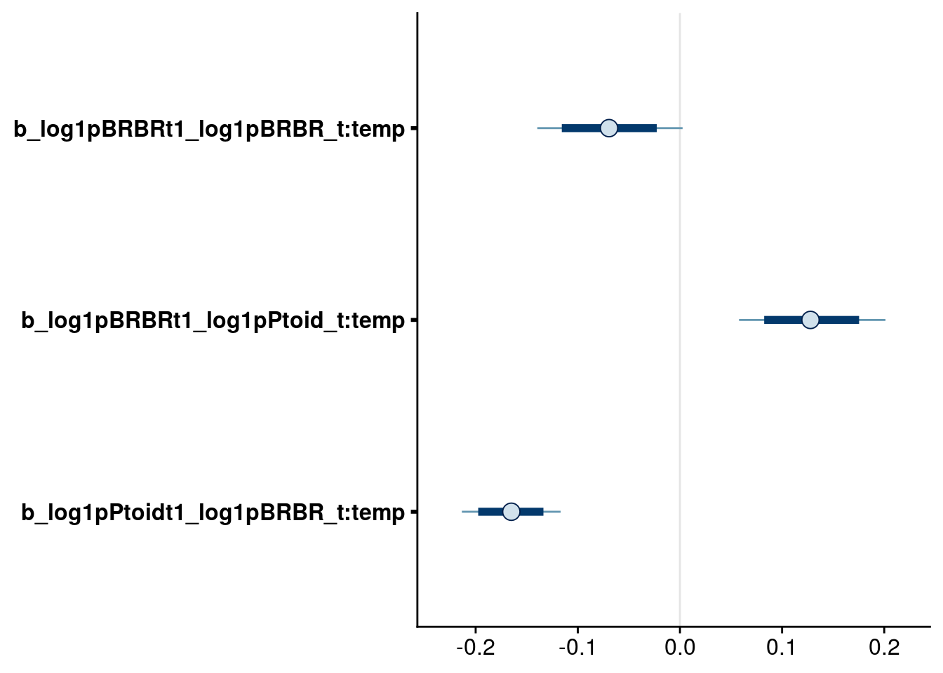

Past versions of reduced-1-summary-1.png

Version	Author	Date
86116c8	mabarbour	2020-06-23

# check main temp effect
bayesplot::mcmc_intervals(reduced.1.brm, regex_pars = "_temp$", prob = 0.80, prob_outer = 0.95) # drop temp effect on LYER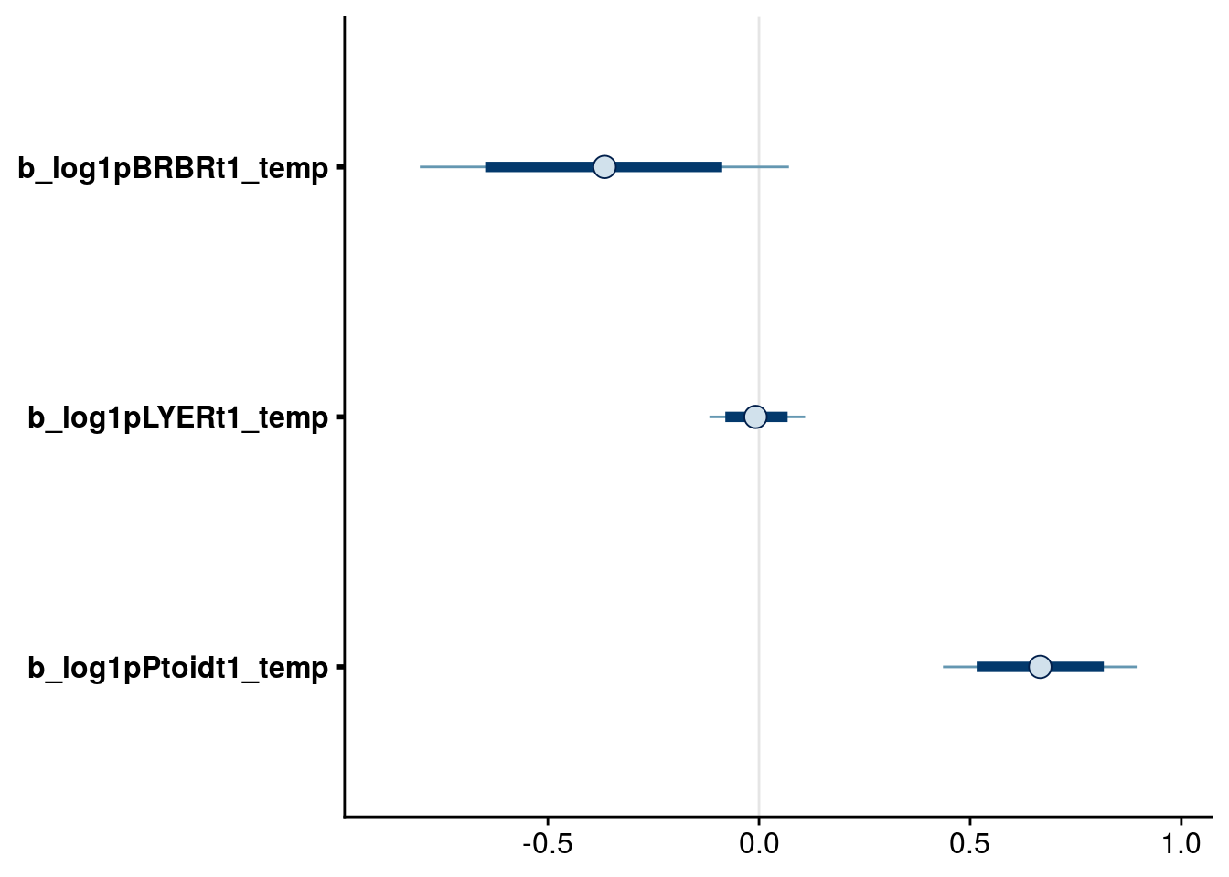

Past versions of reduced-1-summary-2.png

Version	Author	Date
86116c8	mabarbour	2020-06-23

# check highest-order rich effects
bayesplot::mcmc_intervals(reduced.1.brm, regex_pars = ":rich$", prob = 0.80, prob_outer = 0.95) # retain all

Past versions of reduced-1-summary-3.png

Version	Author	Date
86116c8	mabarbour	2020-06-23

# check main rich effect
bayesplot::mcmc_intervals(reduced.1.brm, regex_pars = "_rich$", prob = 0.80, prob_outer = 0.95) # drop rich effect on BRBR, keep others to preserve marginality in higher-order terms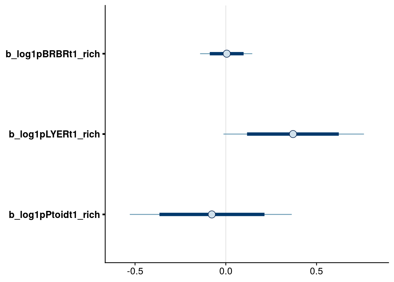

Past versions of reduced-1-summary-4.png

Version	Author	Date
86116c8	mabarbour	2020-06-23

# check biomass effects
bayesplot::mcmc_intervals(reduced.1.brm, regex_pars = "logBiomass_g_t1$", prob = 0.80, prob_outer = 0.95) # drop biomass effect on BRBR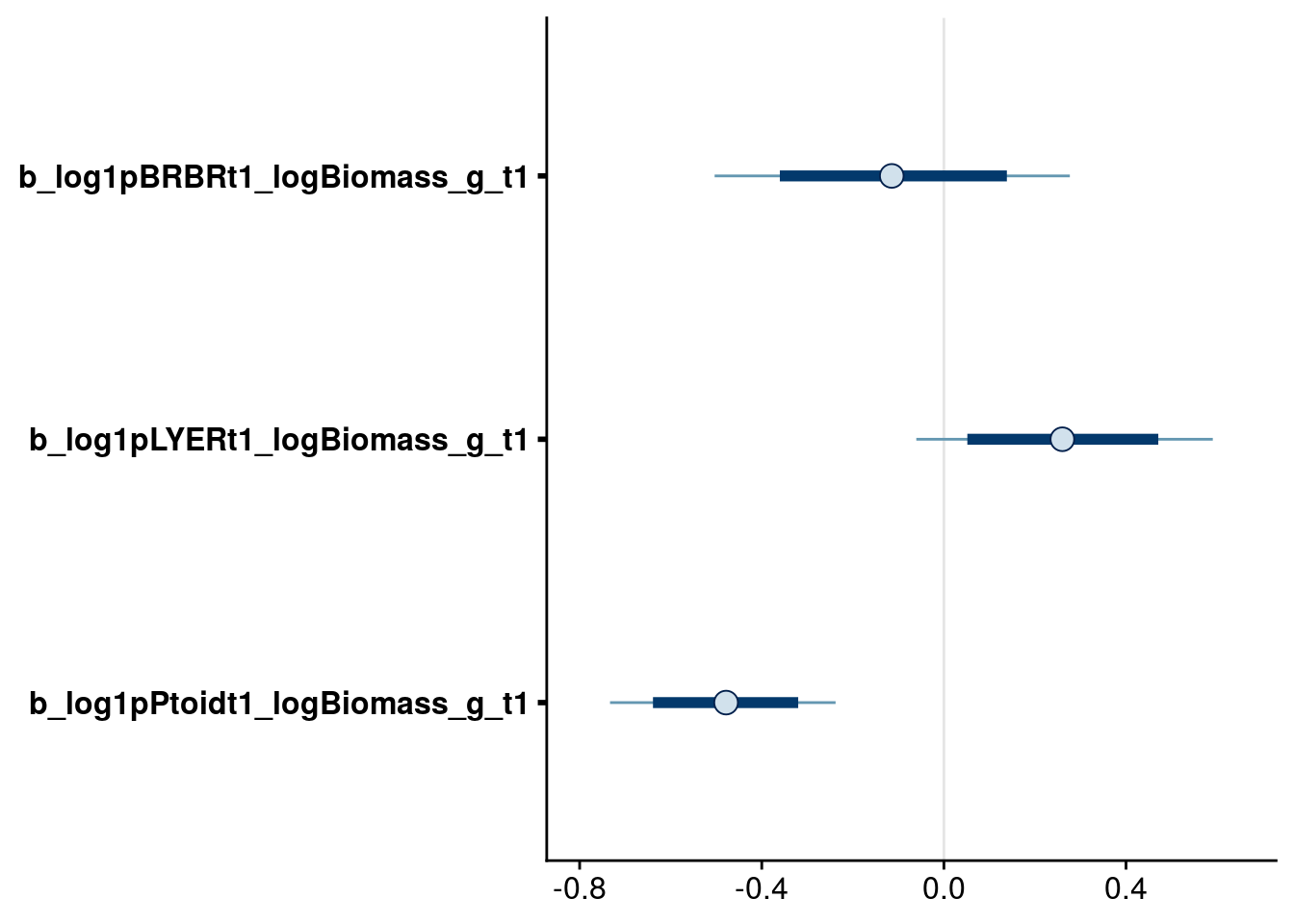

Past versions of reduced-1-summary-5.png

Version	Author	Date
86116c8	mabarbour	2020-06-23

## check interactions (at 20 C in average monoculture)
# BRBR effect
bayesplot::mcmc_intervals(reduced.1.brm, regex_pars = "_log1pBRBR_t$", prob = 0.80, prob_outer = 0.95) # note that I keep intraspecific BRBR effects to preserve marginality with higher-order BRBR:temp effect on BRBR.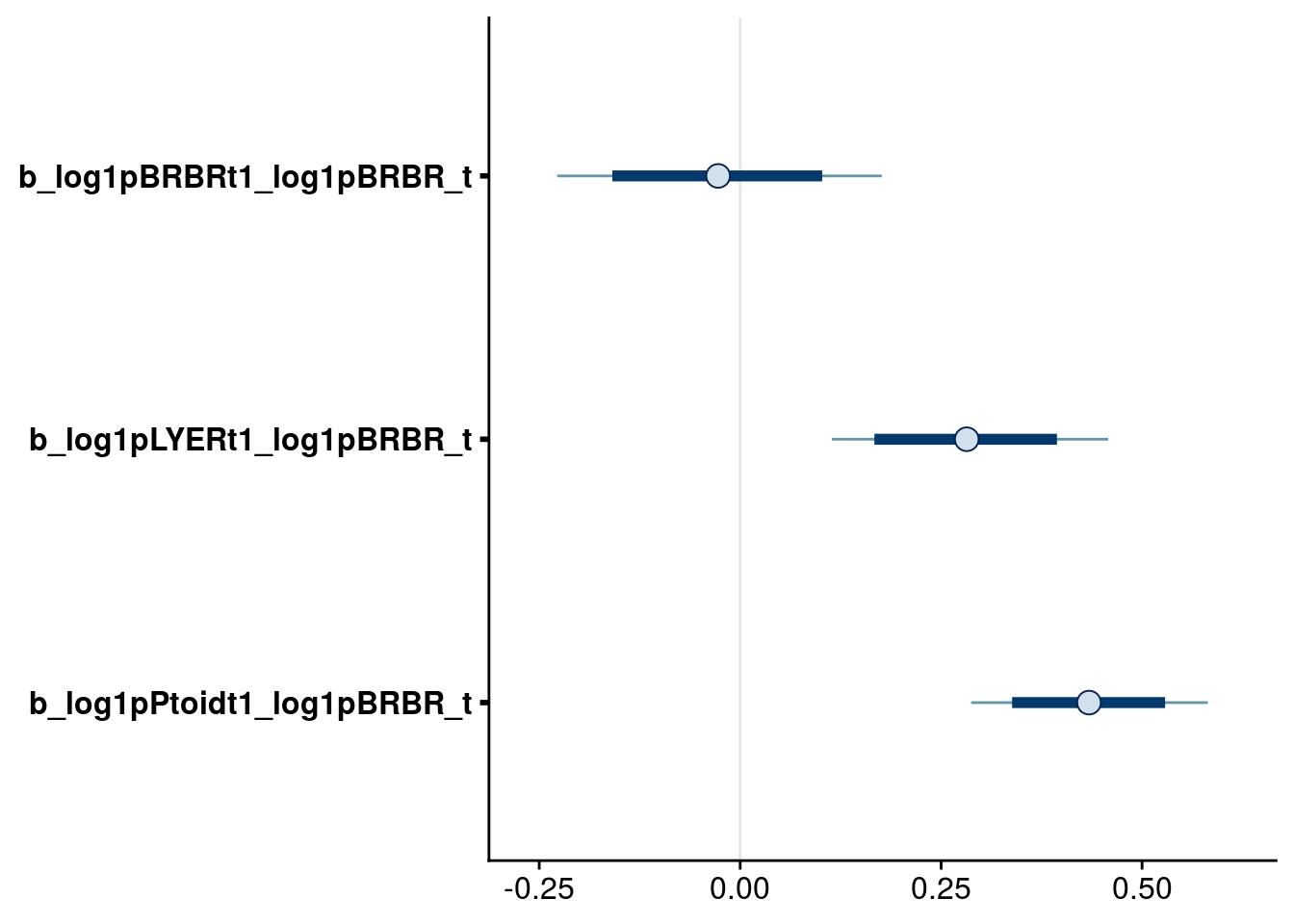

Past versions of reduced-1-summary-6.png

Version	Author	Date
86116c8	mabarbour	2020-06-23

# LYER effect
bayesplot::mcmc_intervals(reduced.1.brm, regex_pars = "_log1pLYER_t$", prob = 0.80, prob_outer = 0.95) # drop LYER effect on BRBR

Past versions of reduced-1-summary-7.png

Version	Author	Date
86116c8	mabarbour	2020-06-23

# Ptoid effect
bayesplot::mcmc_intervals(reduced.1.brm, regex_pars = "_log1pPtoid_t$", prob = 0.80, prob_outer = 0.95) # drop Ptoid effect on itself

Past versions of reduced-1-summary-8.png

Version	Author	Date
86116c8	mabarbour	2020-06-23

Reduced model 2

Drop terms

Based on the above plots, I dropped the following terms:

Effects on BRBR_t1:

• rich
• log1p(LYER_t)
• log(Biomass_g_t1)

Effects on LYER_t1:

• temp

Effects on Ptoid_t1:

• log1p(Ptoid_t)

Refit model

# update formulas
reduced.2.BRBR.bf <- update(reduced.1.BRBR.bf, .~. -rich -log1p(LYER_t) -log(Biomass_g_t1))
reduced.2.LYER.bf <- update(reduced.1.LYER.bf, .~. -temp)
reduced.2.Ptoid.bf <- update(reduced.1.Ptoid.bf, .~. -log1p(Ptoid_t))

# fit new model
reduced.2.brm <- brm(
  data = full_df,
  formula = mvbf(reduced.2.BRBR.bf, reduced.2.LYER.bf, reduced.2.Ptoid.bf),
  iter = 4000,
  prior = c(# growth rates
            set_prior(prior.r.BRBR, class = "b", coef = "intercept", resp = "log1pBRBRt1"),
            set_prior(prior.r.LYER, class = "b", coef = "intercept", resp = "log1pLYERt1"),
            set_prior(prior.r.Ptoid, class = "b", coef = "intercept", resp = "log1pPtoidt1"),
            # intraspecific effects
            set_prior(prior.intra.BRBR, class = "b", coef = "log1pBRBR_t", resp = "log1pBRBRt1"),
            set_prior(prior.intra.LYER, class = "b", coef = "log1pLYER_t", resp = "log1pLYERt1"),
            # negative interspecific effects
            set_prior(prior.BRBRonLYER, class = "b", coef = "log1pBRBR_t", resp = "log1pLYERt1"),
            set_prior(prior.PtoidonBRBR, class = "b", coef = "log1pPtoid_t", resp = "log1pBRBRt1"),
            set_prior(prior.PtoidonLYER, class = "b", coef = "log1pPtoid_t", resp = "log1pLYERt1"),
            # positive interspecific effects
            set_prior(prior.BRBRonPtoid, class = "b", coef = "log1pBRBR_t", resp = "log1pPtoidt1"),
            set_prior(prior.LYERonPtoid, class = "b", coef = "log1pLYER_t", resp = "log1pPtoidt1"),
            # rich effects
            set_prior(prior.rich, class = "b", coef = "rich", resp = "log1pLYERt1"),
            set_prior(prior.rich, class = "b", coef = "rich", resp = "log1pPtoidt1"),  
            set_prior(prior.rich, class = "b", coef = "log1pBRBR_t:rich", resp = "log1pLYERt1"),
            set_prior(prior.rich, class = "b", coef = "log1pBRBR_t:rich", resp = "log1pPtoidt1"),
            set_prior(prior.rich, class = "b", coef = "log1pLYER_t:rich", resp = "log1pPtoidt1"),
            # temp effects
            set_prior(prior.temp, class = "b", coef = "temp", resp = "log1pBRBRt1"),
            set_prior(prior.temp, class = "b", coef = "temp", resp = "log1pPtoidt1"),  
            set_prior(prior.temp, class = "b", coef = "log1pBRBR_t:temp", resp = "log1pBRBRt1"),
            set_prior(prior.temp, class = "b", coef = "log1pBRBR_t:temp", resp = "log1pPtoidt1"),
            set_prior(prior.temp, class = "b", coef = "log1pPtoid_t:temp", resp = "log1pBRBRt1"),
            # biomass effects
            set_prior(prior.AphidBiomass, class = "b", coef = "logBiomass_g_t1", resp = "log1pLYERt1"),
            set_prior(prior.PtoidBiomass, class = "b", coef = "logBiomass_g_t1", resp = "log1pPtoidt1"),
            # random effects
            set_prior(prior.random.effects, class = "sd", resp = "log1pBRBRt1"),
            set_prior(prior.random.effects, class = "sd", resp = "log1pLYERt1"),
            set_prior(prior.random.effects, class = "sd", resp = "log1pPtoidt1")),
  file = "output/reduced.2.brm.rds") 

# print model summary
summary(reduced.2.brm)

 Family: MV(gaussian, gaussian, gaussian) 
  Links: mu = identity; sigma = identity
         mu = identity; sigma = identity
         mu = identity; sigma = identity 
Formula: log1p(BRBR_t1) ~ intercept + log1p(BRBR_t) + log1p(Ptoid_t) + temp + (1 | Cage) + ar(time = Week_match.1p, gr = Cage, p = 1, cov = FALSE) + log1p(BRBR_t):temp + log1p(Ptoid_t):temp + offset(log1p(BRBR_t)) - 1 
         log1p(LYER_t1) ~ intercept + log1p(BRBR_t) + log1p(LYER_t) + log1p(Ptoid_t) + rich + log(Biomass_g_t1) + (1 | Cage) + ar(time = Week_match.1p, gr = Cage, p = 1, cov = FALSE) + log1p(BRBR_t):rich + offset(log1p(LYER_t)) - 1 
         log1p(Ptoid_t1) ~ intercept + log1p(BRBR_t) + log1p(LYER_t) + temp + rich + log(Biomass_g_t1) + (1 | Cage) + ar(time = Week_match.1p, gr = Cage, p = 1, cov = FALSE) + log1p(BRBR_t):temp + log1p(BRBR_t):rich + log1p(LYER_t):rich + offset(log1p(Ptoid_t)) - 1 
   Data: full_df (Number of observations: 264) 
Samples: 4 chains, each with iter = 4000; warmup = 2000; thin = 1;
         total post-warmup samples = 8000

Correlation Structures:
                   Estimate Est.Error l-95% CI u-95% CI Rhat Bulk_ESS Tail_ESS
ar_log1pBRBRt1[1]     -0.44      0.09    -0.61    -0.26 1.00     4459     5718
ar_log1pLYERt1[1]     -0.12      0.10    -0.31     0.07 1.00     6657     6198
ar_log1pPtoidt1[1]    -0.50      0.08    -0.65    -0.34 1.00    12922     7042

Group-Level Effects: 
~Cage (Number of levels: 60) 
                           Estimate Est.Error l-95% CI u-95% CI Rhat Bulk_ESS
sd(log1pBRBRt1_Intercept)      0.24      0.10     0.02     0.42 1.00     1059
sd(log1pLYERt1_Intercept)      0.14      0.09     0.01     0.31 1.00     1762
sd(log1pPtoidt1_Intercept)     0.04      0.03     0.00     0.11 1.00     6103
                           Tail_ESS
sd(log1pBRBRt1_Intercept)      1514
sd(log1pLYERt1_Intercept)      4050
sd(log1pPtoidt1_Intercept)     4428

Population-Level Effects: 
                              Estimate Est.Error l-95% CI u-95% CI Rhat
log1pBRBRt1_intercept             1.47      0.46     0.56     2.38 1.00
log1pBRBRt1_log1pBRBR_t           0.03      0.08    -0.12     0.18 1.00
log1pBRBRt1_log1pPtoid_t         -0.90      0.05    -1.00    -0.79 1.00
log1pBRBRt1_temp                 -0.32      0.22    -0.76     0.10 1.00
log1pBRBRt1_log1pBRBR_t:temp     -0.07      0.04    -0.14     0.00 1.00
log1pBRBRt1_log1pPtoid_t:temp     0.13      0.04     0.06     0.20 1.00
log1pLYERt1_intercept             2.73      0.54     1.67     3.81 1.00
log1pLYERt1_log1pBRBR_t           0.30      0.07     0.16     0.44 1.00
log1pLYERt1_log1pLYER_t          -0.58      0.09    -0.75    -0.42 1.00
log1pLYERt1_log1pPtoid_t         -0.71      0.05    -0.82    -0.62 1.00
log1pLYERt1_rich                  0.38      0.19    -0.01     0.76 1.00
log1pLYERt1_logBiomass_g_t1       0.30      0.15     0.01     0.59 1.00
log1pLYERt1_log1pBRBR_t:rich     -0.07      0.04    -0.15     0.01 1.00
log1pPtoidt1_intercept           -3.16      0.38    -3.90    -2.41 1.00
log1pPtoidt1_log1pBRBR_t          0.44      0.07     0.29     0.58 1.00
log1pPtoidt1_log1pLYER_t          0.32      0.08     0.17     0.47 1.00
log1pPtoidt1_temp                 0.67      0.12     0.44     0.90 1.00
log1pPtoidt1_rich                -0.09      0.23    -0.53     0.36 1.00
log1pPtoidt1_logBiomass_g_t1     -0.48      0.13    -0.72    -0.24 1.00
log1pPtoidt1_log1pBRBR_t:temp    -0.16      0.02    -0.21    -0.12 1.00
log1pPtoidt1_log1pBRBR_t:rich    -0.06      0.04    -0.13     0.01 1.00
log1pPtoidt1_log1pLYER_t:rich     0.07      0.04    -0.01     0.15 1.00
                              Bulk_ESS Tail_ESS
log1pBRBRt1_intercept             5086     5637
log1pBRBRt1_log1pBRBR_t           5879     6205
log1pBRBRt1_log1pPtoid_t          6050     5878
log1pBRBRt1_temp                  5766     5973
log1pBRBRt1_log1pBRBR_t:temp      6211     6633
log1pBRBRt1_log1pPtoid_t:temp     7802     6128
log1pLYERt1_intercept             5579     5882
log1pLYERt1_log1pBRBR_t           8269     6543
log1pLYERt1_log1pLYER_t           5428     6233
log1pLYERt1_log1pPtoid_t          7915     6689
log1pLYERt1_rich                  7974     6381
log1pLYERt1_logBiomass_g_t1      13788     6820
log1pLYERt1_log1pBRBR_t:rich      7925     5781
log1pPtoidt1_intercept            8135     6326
log1pPtoidt1_log1pBRBR_t          7555     6151
log1pPtoidt1_log1pLYER_t          8498     6495
log1pPtoidt1_temp                 6863     6310
log1pPtoidt1_rich                 9087     6182
log1pPtoidt1_logBiomass_g_t1     15373     6540
log1pPtoidt1_log1pBRBR_t:temp     7205     6642
log1pPtoidt1_log1pBRBR_t:rich    10300     6535
log1pPtoidt1_log1pLYER_t:rich     8488     6476

Family Specific Parameters: 
                   Estimate Est.Error l-95% CI u-95% CI Rhat Bulk_ESS Tail_ESS
sigma_log1pBRBRt1      1.12      0.06     1.01     1.23 1.00     3659     5831
sigma_log1pLYERt1      0.92      0.04     0.84     1.01 1.00    10094     6942
sigma_log1pPtoidt1     0.76      0.03     0.70     0.84 1.00    16970     5296

Residual Correlations: 
                                 Estimate Est.Error l-95% CI u-95% CI Rhat
rescor(log1pBRBRt1,log1pLYERt1)      0.51      0.05     0.41     0.60 1.00
rescor(log1pBRBRt1,log1pPtoidt1)    -0.03      0.07    -0.17     0.11 1.00
rescor(log1pLYERt1,log1pPtoidt1)     0.07      0.07    -0.06     0.20 1.00
                                 Bulk_ESS Tail_ESS
rescor(log1pBRBRt1,log1pLYERt1)      8918     6339
rescor(log1pBRBRt1,log1pPtoidt1)    12543     6766
rescor(log1pLYERt1,log1pPtoidt1)    15340     6311

Samples were drawn using sampling(NUTS). For each parameter, Bulk_ESS
and Tail_ESS are effective sample size measures, and Rhat is the potential
scale reduction factor on split chains (at convergence, Rhat = 1).

Inspect credible intervals

# check highest-order temp effects
bayesplot::mcmc_intervals(reduced.2.brm, regex_pars = "_t:temp$", prob = 0.80, prob_outer = 0.95)

Past versions of reduced-2-summary-1.png

Version	Author	Date
86116c8	mabarbour	2020-06-23

# check temp effects on growth rates
bayesplot::mcmc_intervals(reduced.2.brm, regex_pars = "_temp$", prob = 0.80, prob_outer = 0.95)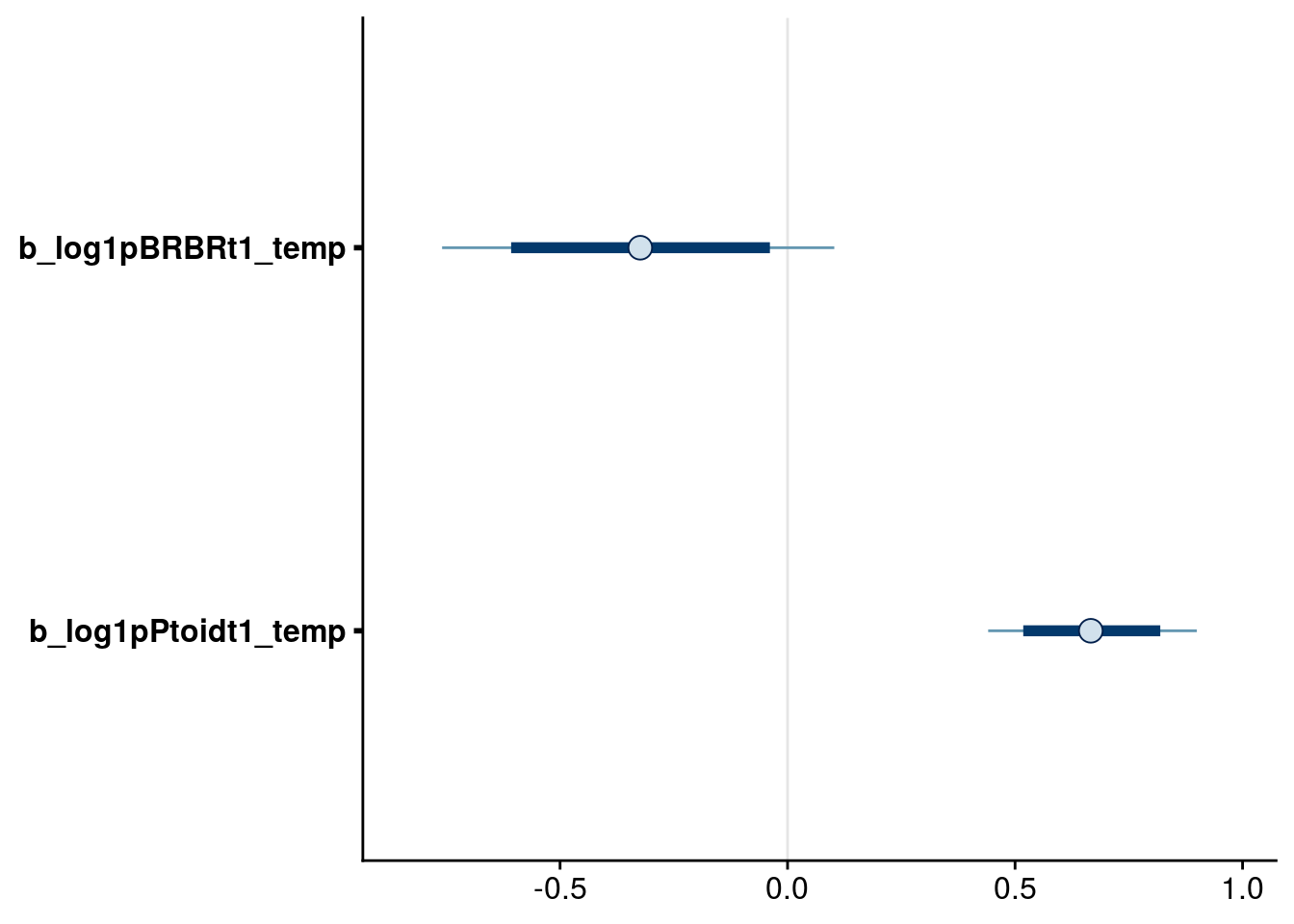

Past versions of reduced-2-summary-2.png

Version	Author	Date
86116c8	mabarbour	2020-06-23

# check highest-order rich effects
bayesplot::mcmc_intervals(reduced.2.brm, regex_pars = "_t:rich$", prob = 0.80, prob_outer = 0.95) # all remaining higher-order rich effects have 95% credible intervals that overlap zero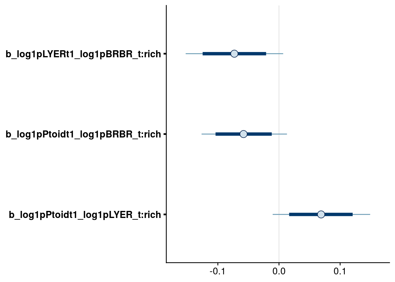

Past versions of reduced-2-summary-3.png

Version	Author	Date
86116c8	mabarbour	2020-06-23

# check rich effects on growth rates
bayesplot::mcmc_intervals(reduced.2.brm, regex_pars = "_rich$", prob = 0.80, prob_outer = 0.95) # note that I keep rich effect on Ptoid to preserve marginality with higher-order rich effect

Past versions of reduced-2-summary-4.png

Version	Author	Date
86116c8	mabarbour	2020-06-23

# check biomass effects
bayesplot::mcmc_intervals(reduced.2.brm, regex_pars = "logBiomass_g_t1$", prob = 0.80, prob_outer = 0.95)

Past versions of reduced-2-summary-5.png

Version	Author	Date
86116c8	mabarbour	2020-06-23

# check intrinsic growth rates (at 20 C in average monoculture)
bayesplot::mcmc_intervals(reduced.2.brm, regex_pars = "intercept$", prob = 0.80, prob_outer = 0.95)

Past versions of reduced-2-summary-6.png

Version	Author	Date
86116c8	mabarbour	2020-06-23

# check interactions (at 20 C in average monoculture)
bayesplot::mcmc_intervals(reduced.2.brm, regex_pars = "_log1pBRBR_t$", prob = 0.80, prob_outer = 0.95) # note that I keep intraspecific BRBR effects to preserve marginality with higher-order BRBR:temp effect on itself.

Past versions of reduced-2-summary-7.png

Version	Author	Date
86116c8	mabarbour	2020-06-23

bayesplot::mcmc_intervals(reduced.2.brm, regex_pars = "_log1pLYER_t$", prob = 0.80, prob_outer = 0.95)

Past versions of reduced-2-summary-8.png

Version	Author	Date
86116c8	mabarbour	2020-06-23

bayesplot::mcmc_intervals(reduced.2.brm, regex_pars = "_log1pPtoid_t$", prob = 0.80, prob_outer = 0.95)

Past versions of reduced-2-summary-9.png

Version	Author	Date
86116c8	mabarbour	2020-06-23

Now, all higher-order terms have 80% credible intervals that do not overlap zero.

Reduced model 3

Drop terms

It is unclear how to progress now, although there are a few terms with less clear effects (still above 80% criteria used previously), including:

Effects on LYER_t1:

• log1p(BRBR_t):rich

Effects on Ptoid_t1:

• log1p(LYER_t):rich
• log1p(BRBR_t):rich

I’m going to try dropping log1p(LYER_t):rich from the previous model.

Refit model

# update formulas
reduced.3.BRBR.bf <- reduced.2.BRBR.bf
reduced.3.LYER.bf <- reduced.2.LYER.bf
reduced.3.Ptoid.bf <- update(reduced.2.Ptoid.bf, .~. -log1p(LYER_t):rich)

# fit new model
reduced.3.brm <- brm(
  data = full_df,
  formula = mvbf(reduced.3.BRBR.bf, reduced.3.LYER.bf, reduced.3.Ptoid.bf),
  iter = 4000,
  prior = c(# growth rates
            set_prior(prior.r.BRBR, class = "b", coef = "intercept", resp = "log1pBRBRt1"),
            set_prior(prior.r.LYER, class = "b", coef = "intercept", resp = "log1pLYERt1"),
            set_prior(prior.r.Ptoid, class = "b", coef = "intercept", resp = "log1pPtoidt1"),
            # intraspecific effects
            set_prior(prior.intra.BRBR, class = "b", coef = "log1pBRBR_t", resp = "log1pBRBRt1"),
            set_prior(prior.intra.LYER, class = "b", coef = "log1pLYER_t", resp = "log1pLYERt1"),
            # negative interspecific effects
            set_prior(prior.BRBRonLYER, class = "b", coef = "log1pBRBR_t", resp = "log1pLYERt1"),
            set_prior(prior.PtoidonBRBR, class = "b", coef = "log1pPtoid_t", resp = "log1pBRBRt1"),
            set_prior(prior.PtoidonLYER, class = "b", coef = "log1pPtoid_t", resp = "log1pLYERt1"),
            # positive interspecific effects
            set_prior(prior.BRBRonPtoid, class = "b", coef = "log1pBRBR_t", resp = "log1pPtoidt1"),
            set_prior(prior.LYERonPtoid, class = "b", coef = "log1pLYER_t", resp = "log1pPtoidt1"),
            # rich effects
            set_prior(prior.rich, class = "b", coef = "rich", resp = "log1pLYERt1"),
            set_prior(prior.rich, class = "b", coef = "rich", resp = "log1pPtoidt1"),
            set_prior(prior.rich, class = "b", coef = "log1pBRBR_t:rich", resp = "log1pLYERt1"),
            set_prior(prior.rich, class = "b", coef = "log1pBRBR_t:rich", resp = "log1pPtoidt1"),
            # temp effects
            set_prior(prior.temp, class = "b", coef = "temp", resp = "log1pBRBRt1"),
            set_prior(prior.temp, class = "b", coef = "temp", resp = "log1pPtoidt1"),  
            set_prior(prior.temp, class = "b", coef = "log1pBRBR_t:temp", resp = "log1pBRBRt1"),
            set_prior(prior.temp, class = "b", coef = "log1pBRBR_t:temp", resp = "log1pPtoidt1"),
            set_prior(prior.temp, class = "b", coef = "log1pPtoid_t:temp", resp = "log1pBRBRt1"),
            # biomass effects
            set_prior(prior.AphidBiomass, class = "b", coef = "logBiomass_g_t1", resp = "log1pLYERt1"),
            set_prior(prior.PtoidBiomass, class = "b", coef = "logBiomass_g_t1", resp = "log1pPtoidt1"),
            # random effects
            set_prior(prior.random.effects, class = "sd", resp = "log1pBRBRt1"),
            set_prior(prior.random.effects, class = "sd", resp = "log1pLYERt1"),
            set_prior(prior.random.effects, class = "sd", resp = "log1pPtoidt1")),
  file = "output/reduced.3.brm.rds") 

# print model summary
summary(reduced.3.brm)

 Family: MV(gaussian, gaussian, gaussian) 
  Links: mu = identity; sigma = identity
         mu = identity; sigma = identity
         mu = identity; sigma = identity 
Formula: log1p(BRBR_t1) ~ intercept + log1p(BRBR_t) + log1p(Ptoid_t) + temp + (1 | Cage) + ar(time = Week_match.1p, gr = Cage, p = 1, cov = FALSE) + log1p(BRBR_t):temp + log1p(Ptoid_t):temp + offset(log1p(BRBR_t)) - 1 
         log1p(LYER_t1) ~ intercept + log1p(BRBR_t) + log1p(LYER_t) + log1p(Ptoid_t) + rich + log(Biomass_g_t1) + (1 | Cage) + ar(time = Week_match.1p, gr = Cage, p = 1, cov = FALSE) + log1p(BRBR_t):rich + offset(log1p(LYER_t)) - 1 
         log1p(Ptoid_t1) ~ intercept + log1p(BRBR_t) + log1p(LYER_t) + temp + rich + log(Biomass_g_t1) + (1 | Cage) + ar(time = Week_match.1p, gr = Cage, p = 1, cov = FALSE) + log1p(BRBR_t):temp + log1p(BRBR_t):rich + offset(log1p(Ptoid_t)) - 1 
   Data: full_df (Number of observations: 264) 
Samples: 4 chains, each with iter = 4000; warmup = 2000; thin = 1;
         total post-warmup samples = 8000

Correlation Structures:
                   Estimate Est.Error l-95% CI u-95% CI Rhat Bulk_ESS Tail_ESS
ar_log1pBRBRt1[1]     -0.44      0.09    -0.62    -0.26 1.00     3843     6249
ar_log1pLYERt1[1]     -0.12      0.10    -0.30     0.07 1.00     6062     6048
ar_log1pPtoidt1[1]    -0.50      0.08    -0.66    -0.34 1.00     9303     5957

Group-Level Effects: 
~Cage (Number of levels: 60) 
                           Estimate Est.Error l-95% CI u-95% CI Rhat Bulk_ESS
sd(log1pBRBRt1_Intercept)      0.24      0.10     0.03     0.43 1.00     1093
sd(log1pLYERt1_Intercept)      0.14      0.08     0.01     0.31 1.00     1737
sd(log1pPtoidt1_Intercept)     0.04      0.03     0.00     0.11 1.00     5475
                           Tail_ESS
sd(log1pBRBRt1_Intercept)      1963
sd(log1pLYERt1_Intercept)      2994
sd(log1pPtoidt1_Intercept)     4459

Population-Level Effects: 
                              Estimate Est.Error l-95% CI u-95% CI Rhat
log1pBRBRt1_intercept             1.48      0.46     0.59     2.40 1.00
log1pBRBRt1_log1pBRBR_t           0.03      0.08    -0.12     0.18 1.00
log1pBRBRt1_log1pPtoid_t         -0.90      0.05    -1.01    -0.79 1.00
log1pBRBRt1_temp                 -0.32      0.21    -0.75     0.09 1.00
log1pBRBRt1_log1pBRBR_t:temp     -0.07      0.04    -0.14     0.00 1.00
log1pBRBRt1_log1pPtoid_t:temp     0.13      0.04     0.06     0.20 1.00
log1pLYERt1_intercept             2.74      0.54     1.70     3.79 1.00
log1pLYERt1_log1pBRBR_t           0.30      0.07     0.16     0.44 1.00
log1pLYERt1_log1pLYER_t          -0.58      0.08    -0.76    -0.42 1.00
log1pLYERt1_log1pPtoid_t         -0.72      0.05    -0.82    -0.61 1.00
log1pLYERt1_rich                  0.38      0.20    -0.01     0.76 1.00
log1pLYERt1_logBiomass_g_t1       0.30      0.15     0.01     0.58 1.00
log1pLYERt1_log1pBRBR_t:rich     -0.07      0.04    -0.15     0.01 1.00
log1pPtoidt1_intercept           -3.40      0.36    -4.10    -2.70 1.00
log1pPtoidt1_log1pBRBR_t          0.40      0.07     0.26     0.54 1.00
log1pPtoidt1_log1pLYER_t          0.40      0.06     0.28     0.52 1.00
log1pPtoidt1_temp                 0.65      0.12     0.42     0.88 1.00
log1pPtoidt1_rich                 0.18      0.17    -0.14     0.51 1.00
log1pPtoidt1_logBiomass_g_t1     -0.49      0.12    -0.73    -0.25 1.00
log1pPtoidt1_log1pBRBR_t:temp    -0.16      0.02    -0.21    -0.12 1.00
log1pPtoidt1_log1pBRBR_t:rich    -0.04      0.03    -0.11     0.03 1.00
                              Bulk_ESS Tail_ESS
log1pBRBRt1_intercept             4031     5396
log1pBRBRt1_log1pBRBR_t           5076     5933
log1pBRBRt1_log1pPtoid_t          4404     5489
log1pBRBRt1_temp                  4269     5087
log1pBRBRt1_log1pBRBR_t:temp      4835     5526
log1pBRBRt1_log1pPtoid_t:temp     5559     5716
log1pLYERt1_intercept             4928     5071
log1pLYERt1_log1pBRBR_t           6863     6090
log1pLYERt1_log1pLYER_t           4690     5519
log1pLYERt1_log1pPtoid_t          5838     6263
log1pLYERt1_rich                  5960     5619
log1pLYERt1_logBiomass_g_t1      10203     6204
log1pLYERt1_log1pBRBR_t:rich      5916     5539
log1pPtoidt1_intercept            6774     5597
log1pPtoidt1_log1pBRBR_t          5859     5853
log1pPtoidt1_log1pLYER_t          9124     4922
log1pPtoidt1_temp                 5450     5166
log1pPtoidt1_rich                 6268     5242
log1pPtoidt1_logBiomass_g_t1     10418     6393
log1pPtoidt1_log1pBRBR_t:temp     5668     5454
log1pPtoidt1_log1pBRBR_t:rich     6250     5271

Family Specific Parameters: 
                   Estimate Est.Error l-95% CI u-95% CI Rhat Bulk_ESS Tail_ESS
sigma_log1pBRBRt1      1.11      0.06     1.00     1.23 1.00     3337     4780
sigma_log1pLYERt1      0.92      0.04     0.84     1.01 1.00     7022     5783
sigma_log1pPtoidt1     0.77      0.03     0.70     0.84 1.00    10358     5625

Residual Correlations: 
                                 Estimate Est.Error l-95% CI u-95% CI Rhat
rescor(log1pBRBRt1,log1pLYERt1)      0.51      0.05     0.41     0.61 1.00
rescor(log1pBRBRt1,log1pPtoidt1)    -0.03      0.07    -0.17     0.11 1.00
rescor(log1pLYERt1,log1pPtoidt1)     0.07      0.06    -0.05     0.20 1.00
                                 Bulk_ESS Tail_ESS
rescor(log1pBRBRt1,log1pLYERt1)      6159     5704
rescor(log1pBRBRt1,log1pPtoidt1)     9267     6352
rescor(log1pLYERt1,log1pPtoidt1)    11538     6463

Samples were drawn using sampling(NUTS). For each parameter, Bulk_ESS
and Tail_ESS are effective sample size measures, and Rhat is the potential
scale reduction factor on split chains (at convergence, Rhat = 1).

Inspect credible intervals

Note that this is the final model used to assess the structural stability of the initial food web and the dominant food chain, so I illustrate the credible intervals of its modelled parameters.

# check highest-order temp effects
bayesplot::mcmc_intervals(reduced.3.brm, regex_pars = "_t:temp$", prob = 0.80, prob_outer = 0.95)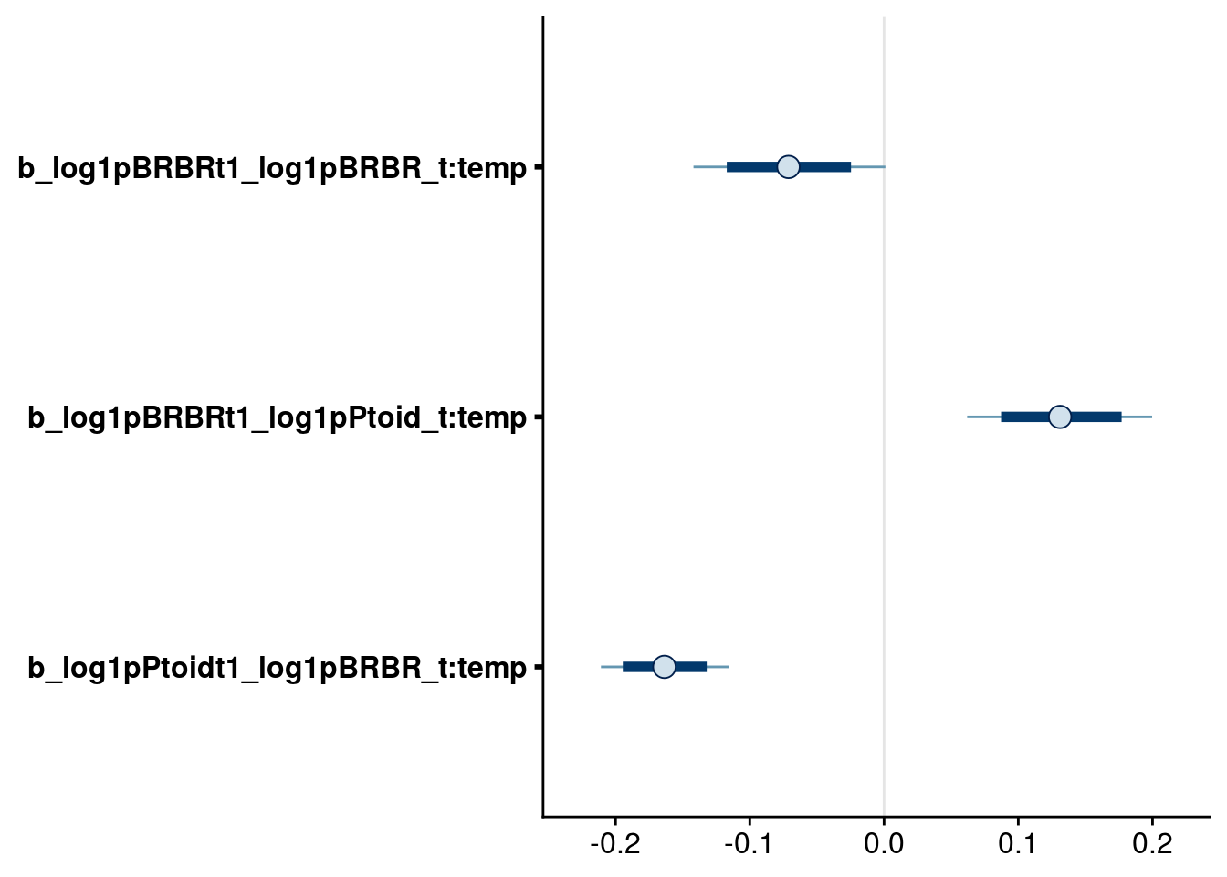

Past versions of reduced-3-summary-1.png

Version	Author	Date
86116c8	mabarbour	2020-06-23

# check highest-order rich effects
bayesplot::mcmc_intervals(reduced.3.brm, regex_pars = "_t:rich$", prob = 0.80, prob_outer = 0.95) # higher-order BRBR:rich effect on Ptoid no longer meets 80% cutoff.

Past versions of reduced-3-summary-2.png

Version	Author	Date
86116c8	mabarbour	2020-06-23

# check temp effects on growth rates
bayesplot::mcmc_intervals(reduced.3.brm, regex_pars = "_temp$", prob = 0.80, prob_outer = 0.95)

Past versions of reduced-3-summary-3.png

Version	Author	Date
86116c8	mabarbour	2020-06-23

# check rich effects on growth rates
bayesplot::mcmc_intervals(reduced.3.brm, regex_pars = "_rich$", prob = 0.80, prob_outer = 0.95)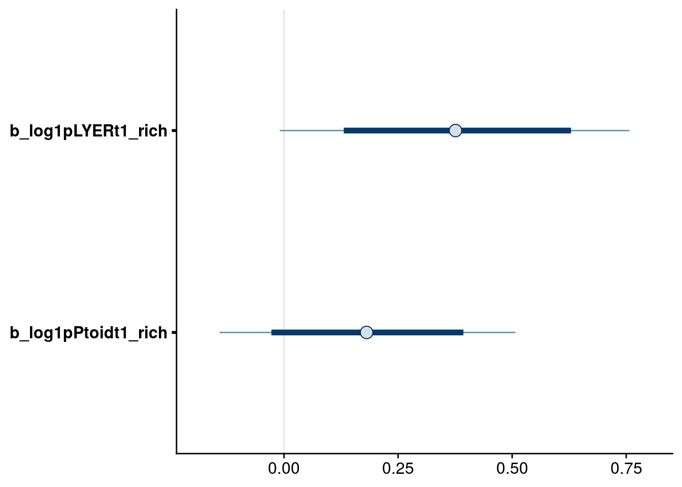

Past versions of reduced-3-summary-4.png

Version	Author	Date
86116c8	mabarbour	2020-06-23

# check biomass effects
bayesplot::mcmc_intervals(reduced.3.brm, regex_pars = "logBiomass_g_t1$", prob = 0.80, prob_outer = 0.95)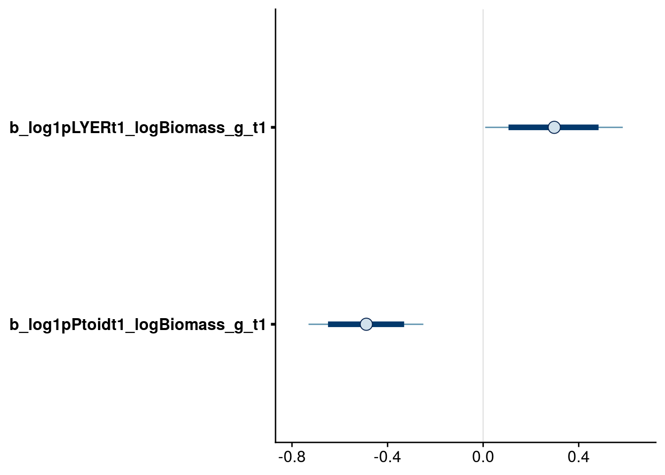

Past versions of reduced-3-summary-5.png

Version	Author	Date
86116c8	mabarbour	2020-06-23

# check intrinsic growth rates (at 20 C in average monoculture)
bayesplot::mcmc_intervals(reduced.3.brm, regex_pars = "intercept$", prob = 0.80, prob_outer = 0.95)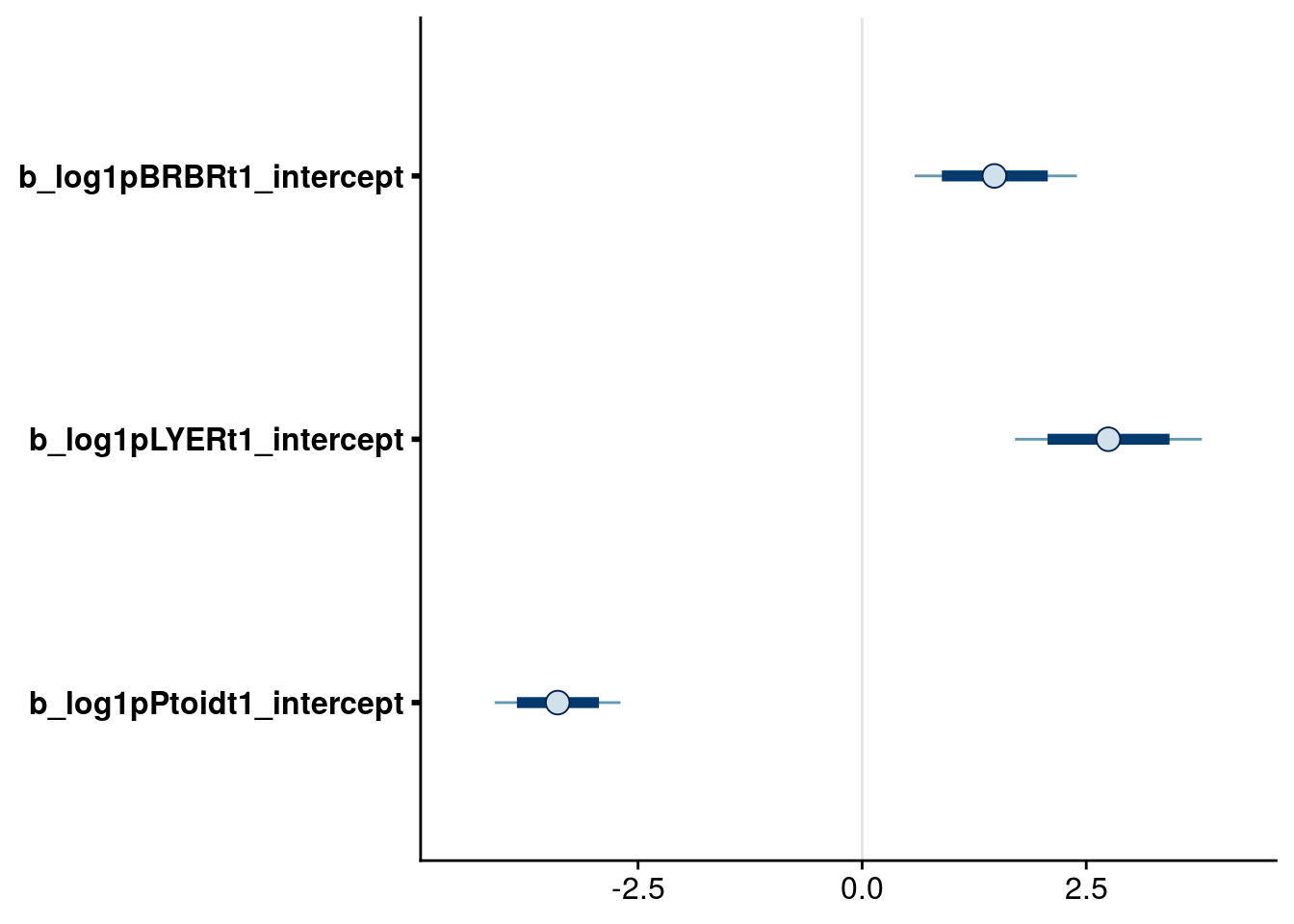

Past versions of reduced-3-summary-6.png

Version	Author	Date
86116c8	mabarbour	2020-06-23

# check interactions (at 20 C in average monoculture)
bayesplot::mcmc_intervals(reduced.3.brm, regex_pars = "_log1pBRBR_t$", prob = 0.80, prob_outer = 0.95)

Past versions of reduced-3-summary-7.png

Version	Author	Date
86116c8	mabarbour	2020-06-23

bayesplot::mcmc_intervals(reduced.3.brm, regex_pars = "_log1pLYER_t$", prob = 0.80, prob_outer = 0.95)

Past versions of reduced-3-summary-8.png

Version	Author	Date
86116c8	mabarbour	2020-06-23

bayesplot::mcmc_intervals(reduced.3.brm, regex_pars = "_log1pPtoid_t$", prob = 0.80, prob_outer = 0.95)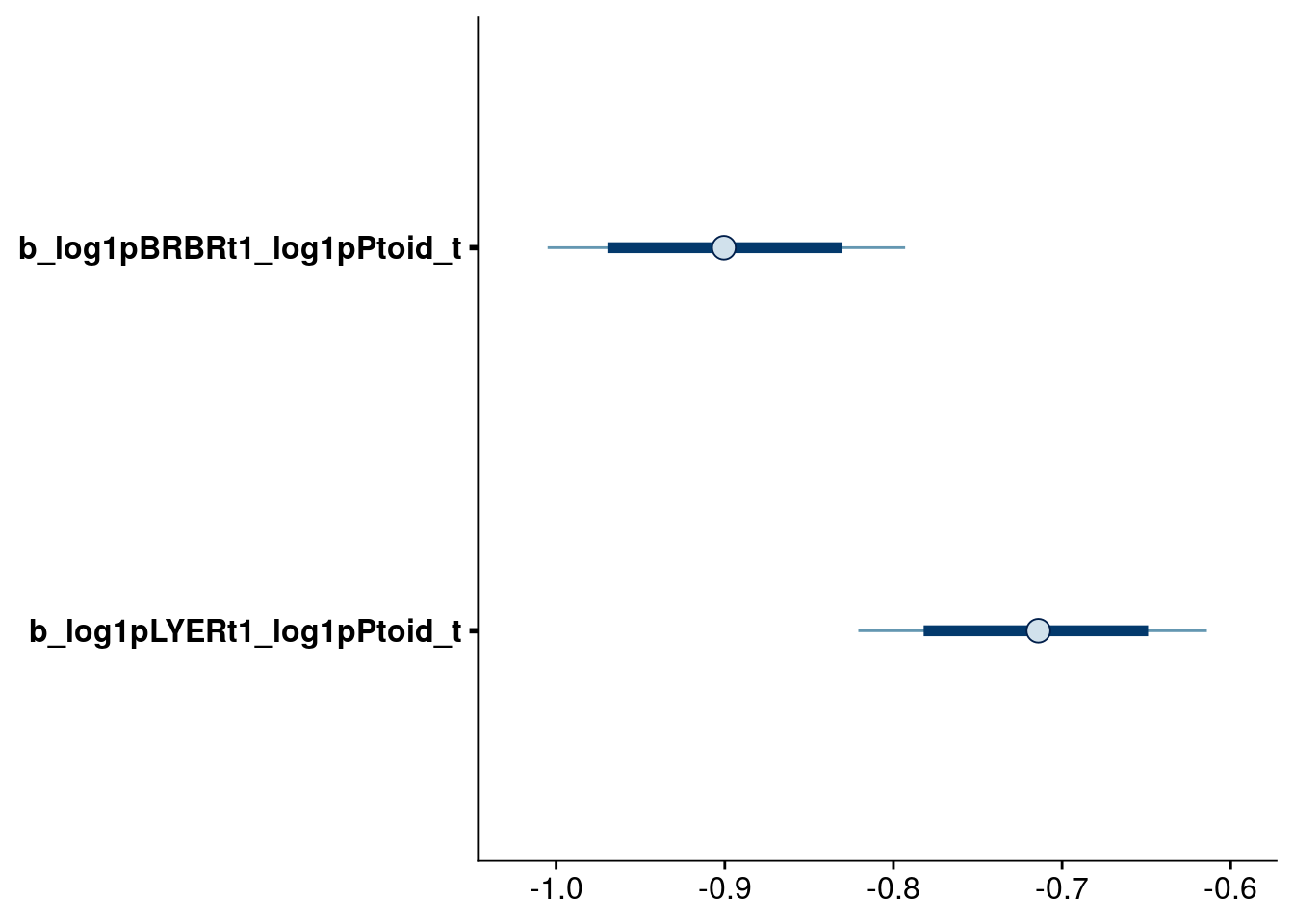

Past versions of reduced-3-summary-9.png

Version	Author	Date
86116c8	mabarbour	2020-06-23

Reduced model 4

Drop terms

Now try dropping log1p(BRBR_t):rich effect on Ptoid_t1 instead.

Refit model

# update formulas
# note that I'm updating model 2, not model 3
reduced.4.BRBR.bf <- reduced.2.BRBR.bf
reduced.4.LYER.bf <- reduced.2.LYER.bf
reduced.4.Ptoid.bf <- update(reduced.2.Ptoid.bf, .~. -log1p(BRBR_t):rich)

# fit new model
reduced.4.brm <- brm(
  data = full_df,
  formula = mvbf(reduced.4.BRBR.bf, reduced.4.LYER.bf, reduced.4.Ptoid.bf),
  iter = 4000,
  prior = c(# growth rates
            set_prior(prior.r.BRBR, class = "b", coef = "intercept", resp = "log1pBRBRt1"),
            set_prior(prior.r.LYER, class = "b", coef = "intercept", resp = "log1pLYERt1"),
            set_prior(prior.r.Ptoid, class = "b", coef = "intercept", resp = "log1pPtoidt1"),
            # intraspecific effects
            set_prior(prior.intra.BRBR, class = "b", coef = "log1pBRBR_t", resp = "log1pBRBRt1"),
            set_prior(prior.intra.LYER, class = "b", coef = "log1pLYER_t", resp = "log1pLYERt1"),
            # negative interspecific effects
            set_prior(prior.BRBRonLYER, class = "b", coef = "log1pBRBR_t", resp = "log1pLYERt1"),
            set_prior(prior.PtoidonBRBR, class = "b", coef = "log1pPtoid_t", resp = "log1pBRBRt1"),
            set_prior(prior.PtoidonLYER, class = "b", coef = "log1pPtoid_t", resp = "log1pLYERt1"),
            # positive interspecific effects
            set_prior(prior.BRBRonPtoid, class = "b", coef = "log1pBRBR_t", resp = "log1pPtoidt1"),
            set_prior(prior.LYERonPtoid, class = "b", coef = "log1pLYER_t", resp = "log1pPtoidt1"),
            # rich effects
            set_prior(prior.rich, class = "b", coef = "rich", resp = "log1pLYERt1"),
            set_prior(prior.rich, class = "b", coef = "rich", resp = "log1pPtoidt1"),
            set_prior(prior.rich, class = "b", coef = "log1pBRBR_t:rich", resp = "log1pLYERt1"),
            set_prior(prior.rich, class = "b", coef = "log1pLYER_t:rich", resp = "log1pPtoidt1"),
            # temp effects
            set_prior(prior.temp, class = "b", coef = "temp", resp = "log1pBRBRt1"),
            set_prior(prior.temp, class = "b", coef = "temp", resp = "log1pPtoidt1"),  
            set_prior(prior.temp, class = "b", coef = "log1pBRBR_t:temp", resp = "log1pBRBRt1"),
            set_prior(prior.temp, class = "b", coef = "log1pBRBR_t:temp", resp = "log1pPtoidt1"),
            set_prior(prior.temp, class = "b", coef = "log1pPtoid_t:temp", resp = "log1pBRBRt1"),
            # biomass effects
            set_prior(prior.AphidBiomass, class = "b", coef = "logBiomass_g_t1", resp = "log1pLYERt1"),
            set_prior(prior.PtoidBiomass, class = "b", coef = "logBiomass_g_t1", resp = "log1pPtoidt1"),
            # random effects
            set_prior(prior.random.effects, class = "sd", resp = "log1pBRBRt1"),
            set_prior(prior.random.effects, class = "sd", resp = "log1pLYERt1"),
            set_prior(prior.random.effects, class = "sd", resp = "log1pPtoidt1")),
  file = "output/reduced.4.brm.rds") 

# print model summary
summary(reduced.4.brm)

 Family: MV(gaussian, gaussian, gaussian) 
  Links: mu = identity; sigma = identity
         mu = identity; sigma = identity
         mu = identity; sigma = identity 
Formula: log1p(BRBR_t1) ~ intercept + log1p(BRBR_t) + log1p(Ptoid_t) + temp + (1 | Cage) + ar(time = Week_match.1p, gr = Cage, p = 1, cov = FALSE) + log1p(BRBR_t):temp + log1p(Ptoid_t):temp + offset(log1p(BRBR_t)) - 1 
         log1p(LYER_t1) ~ intercept + log1p(BRBR_t) + log1p(LYER_t) + log1p(Ptoid_t) + rich + log(Biomass_g_t1) + (1 | Cage) + ar(time = Week_match.1p, gr = Cage, p = 1, cov = FALSE) + log1p(BRBR_t):rich + offset(log1p(LYER_t)) - 1 
         log1p(Ptoid_t1) ~ intercept + log1p(BRBR_t) + log1p(LYER_t) + temp + rich + log(Biomass_g_t1) + (1 | Cage) + ar(time = Week_match.1p, gr = Cage, p = 1, cov = FALSE) + log1p(BRBR_t):temp + log1p(LYER_t):rich + offset(log1p(Ptoid_t)) - 1 
   Data: full_df (Number of observations: 264) 
Samples: 4 chains, each with iter = 4000; warmup = 2000; thin = 1;
         total post-warmup samples = 8000

Correlation Structures:
                   Estimate Est.Error l-95% CI u-95% CI Rhat Bulk_ESS Tail_ESS
ar_log1pBRBRt1[1]     -0.45      0.09    -0.62    -0.26 1.00     4747     6121
ar_log1pLYERt1[1]     -0.12      0.10    -0.30     0.07 1.00     6624     6554
ar_log1pPtoidt1[1]    -0.50      0.08    -0.66    -0.34 1.00    13790     6929

Group-Level Effects: 
~Cage (Number of levels: 60) 
                           Estimate Est.Error l-95% CI u-95% CI Rhat Bulk_ESS
sd(log1pBRBRt1_Intercept)      0.25      0.10     0.03     0.43 1.00     1349
sd(log1pLYERt1_Intercept)      0.13      0.09     0.01     0.31 1.00     1988
sd(log1pPtoidt1_Intercept)     0.04      0.03     0.00     0.11 1.00     5637
                           Tail_ESS
sd(log1pBRBRt1_Intercept)      2018
sd(log1pLYERt1_Intercept)      3924
sd(log1pPtoidt1_Intercept)     4762

Population-Level Effects: 
                              Estimate Est.Error l-95% CI u-95% CI Rhat
log1pBRBRt1_intercept             1.48      0.47     0.55     2.38 1.00
log1pBRBRt1_log1pBRBR_t           0.03      0.08    -0.12     0.18 1.00
log1pBRBRt1_log1pPtoid_t         -0.90      0.05    -1.01    -0.79 1.00
log1pBRBRt1_temp                 -0.32      0.22    -0.74     0.11 1.00
log1pBRBRt1_log1pBRBR_t:temp     -0.07      0.04    -0.14     0.00 1.00
log1pBRBRt1_log1pPtoid_t:temp     0.13      0.04     0.06     0.20 1.00
log1pLYERt1_intercept             2.76      0.55     1.70     3.84 1.00
log1pLYERt1_log1pBRBR_t           0.29      0.07     0.16     0.43 1.00
log1pLYERt1_log1pLYER_t          -0.58      0.08    -0.75    -0.42 1.00
log1pLYERt1_log1pPtoid_t         -0.71      0.05    -0.82    -0.62 1.00
log1pLYERt1_rich                  0.35      0.20    -0.03     0.73 1.00
log1pLYERt1_logBiomass_g_t1       0.30      0.15     0.00     0.59 1.00
log1pLYERt1_log1pBRBR_t:rich     -0.07      0.04    -0.15     0.01 1.00
log1pPtoidt1_intercept           -3.04      0.38    -3.78    -2.31 1.00
log1pPtoidt1_log1pBRBR_t          0.37      0.06     0.25     0.49 1.00
log1pPtoidt1_log1pLYER_t          0.35      0.07     0.21     0.50 1.00
log1pPtoidt1_temp                 0.69      0.12     0.46     0.92 1.00
log1pPtoidt1_rich                -0.24      0.20    -0.64     0.16 1.00
log1pPtoidt1_logBiomass_g_t1     -0.47      0.13    -0.72    -0.22 1.00
log1pPtoidt1_log1pBRBR_t:temp    -0.17      0.02    -0.22    -0.12 1.00
log1pPtoidt1_log1pLYER_t:rich     0.05      0.04    -0.03     0.12 1.00
                              Bulk_ESS Tail_ESS
log1pBRBRt1_intercept             4795     5644
log1pBRBRt1_log1pBRBR_t           5547     6061
log1pBRBRt1_log1pPtoid_t          6059     5661
log1pBRBRt1_temp                  5384     5468
log1pBRBRt1_log1pBRBR_t:temp      5527     6037
log1pBRBRt1_log1pPtoid_t:temp     7658     5942
log1pLYERt1_intercept             6093     5968
log1pLYERt1_log1pBRBR_t           7264     5423
log1pLYERt1_log1pLYER_t           6798     6071
log1pLYERt1_log1pPtoid_t          8210     7051
log1pLYERt1_rich                  6865     5295
log1pLYERt1_logBiomass_g_t1      12129     5633
log1pLYERt1_log1pBRBR_t:rich      6788     5810
log1pPtoidt1_intercept            7589     6544
log1pPtoidt1_log1pBRBR_t          7144     6251
log1pPtoidt1_log1pLYER_t          7816     6150
log1pPtoidt1_temp                 6741     5841
log1pPtoidt1_rich                 7441     6258
log1pPtoidt1_logBiomass_g_t1     13801     6286
log1pPtoidt1_log1pBRBR_t:temp     7264     5826
log1pPtoidt1_log1pLYER_t:rich     7523     6249

Family Specific Parameters: 
                   Estimate Est.Error l-95% CI u-95% CI Rhat Bulk_ESS Tail_ESS
sigma_log1pBRBRt1      1.11      0.06     1.00     1.23 1.00     3881     6502
sigma_log1pLYERt1      0.92      0.04     0.84     1.01 1.00     8520     6614
sigma_log1pPtoidt1     0.77      0.03     0.70     0.84 1.00    15660     5320

Residual Correlations: 
                                 Estimate Est.Error l-95% CI u-95% CI Rhat
rescor(log1pBRBRt1,log1pLYERt1)      0.51      0.05     0.41     0.61 1.00
rescor(log1pBRBRt1,log1pPtoidt1)    -0.02      0.07    -0.16     0.12 1.00
rescor(log1pLYERt1,log1pPtoidt1)     0.08      0.07    -0.05     0.20 1.00
                                 Bulk_ESS Tail_ESS
rescor(log1pBRBRt1,log1pLYERt1)      9039     6468
rescor(log1pBRBRt1,log1pPtoidt1)    11723     6652
rescor(log1pLYERt1,log1pPtoidt1)    13786     5964

Samples were drawn using sampling(NUTS). For each parameter, Bulk_ESS
and Tail_ESS are effective sample size measures, and Rhat is the potential
scale reduction factor on split chains (at convergence, Rhat = 1).

Inspect credible intervals

# check highest-order rich effects
bayesplot::mcmc_intervals(reduced.4.brm, regex_pars = "_t:rich$", prob = 0.80, prob_outer = 0.95) # higher-order LYER:rich effect on Ptoid no longer meets 80% cutoff.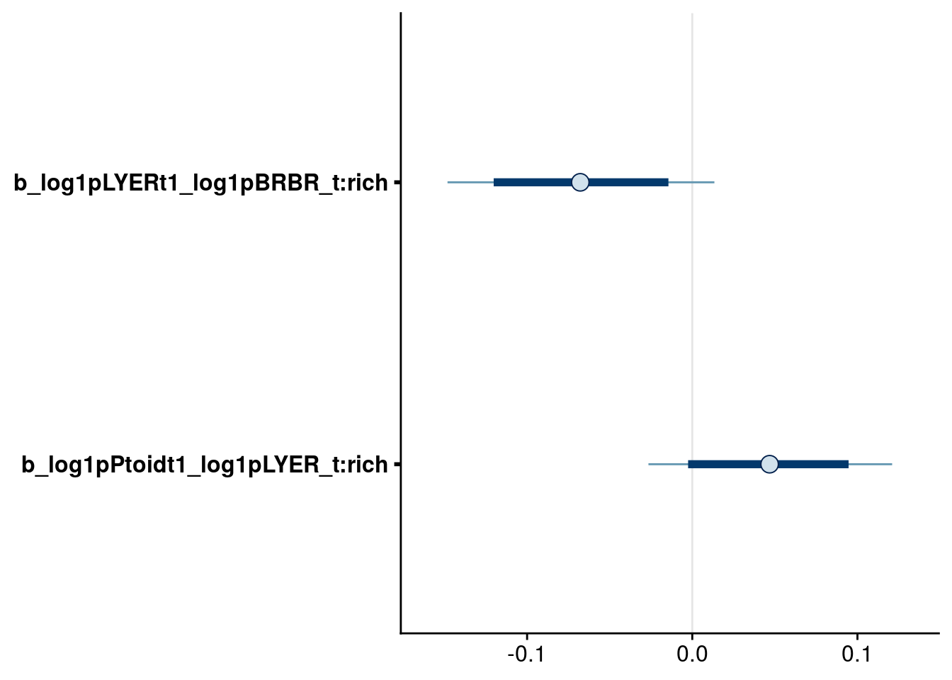

Past versions of reduced-4-summary-1.png

Version	Author	Date
86116c8	mabarbour	2020-06-23

Reduced model 5

Drop terms

For both reduced model 3 and 4, once I drop the higher-order interaction with rich, the other higher-order term doesn’t meet the 80% interval cutoff, so I will try dropping both from the model.

After dropping this term, it also appears that rich effect on Ptoid intrinsic growth rate is no longer needed (80% interval criterion, model not shown), so I will drop that now too.

This model effectively removes all of the rich effects on Ptoid_t1.

Refit model

# update formulas
# note that I'm updating model 2
reduced.5.BRBR.bf <- reduced.2.BRBR.bf
reduced.5.LYER.bf <- reduced.2.LYER.bf
reduced.5.Ptoid.bf <- update(reduced.2.Ptoid.bf, .~. -log1p(BRBR_t):rich -log1p(LYER_t):rich -rich)

# fit new model
reduced.5.brm <- brm(
  data = full_df,
  formula = mvbf(reduced.5.BRBR.bf, reduced.5.LYER.bf, reduced.5.Ptoid.bf),
  iter = 4000,
  prior = c(# growth rates
            set_prior(prior.r.BRBR, class = "b", coef = "intercept", resp = "log1pBRBRt1"),
            set_prior(prior.r.LYER, class = "b", coef = "intercept", resp = "log1pLYERt1"),
            set_prior(prior.r.Ptoid, class = "b", coef = "intercept", resp = "log1pPtoidt1"),
            # intraspecific effects
            set_prior(prior.intra.BRBR, class = "b", coef = "log1pBRBR_t", resp = "log1pBRBRt1"),
            set_prior(prior.intra.LYER, class = "b", coef = "log1pLYER_t", resp = "log1pLYERt1"),
            # negative interspecific effects
            set_prior(prior.BRBRonLYER, class = "b", coef = "log1pBRBR_t", resp = "log1pLYERt1"),
            set_prior(prior.PtoidonBRBR, class = "b", coef = "log1pPtoid_t", resp = "log1pBRBRt1"),
            set_prior(prior.PtoidonLYER, class = "b", coef = "log1pPtoid_t", resp = "log1pLYERt1"),
            # positive interspecific effects
            set_prior(prior.BRBRonPtoid, class = "b", coef = "log1pBRBR_t", resp = "log1pPtoidt1"),
            set_prior(prior.LYERonPtoid, class = "b", coef = "log1pLYER_t", resp = "log1pPtoidt1"),
            # rich effects
            set_prior(prior.rich, class = "b", coef = "rich", resp = "log1pLYERt1"),
            set_prior(prior.rich, class = "b", coef = "log1pBRBR_t:rich", resp = "log1pLYERt1"),
            # temp effects
            set_prior(prior.temp, class = "b", coef = "temp", resp = "log1pBRBRt1"),
            set_prior(prior.temp, class = "b", coef = "temp", resp = "log1pPtoidt1"),  
            set_prior(prior.temp, class = "b", coef = "log1pBRBR_t:temp", resp = "log1pBRBRt1"),
            set_prior(prior.temp, class = "b", coef = "log1pBRBR_t:temp", resp = "log1pPtoidt1"),
            set_prior(prior.temp, class = "b", coef = "log1pPtoid_t:temp", resp = "log1pBRBRt1"),
            # biomass effects
            set_prior(prior.AphidBiomass, class = "b", coef = "logBiomass_g_t1", resp = "log1pLYERt1"),
            set_prior(prior.PtoidBiomass, class = "b", coef = "logBiomass_g_t1", resp = "log1pPtoidt1"),
            # random effects
            set_prior(prior.random.effects, class = "sd", resp = "log1pBRBRt1"),
            set_prior(prior.random.effects, class = "sd", resp = "log1pLYERt1"),
            set_prior(prior.random.effects, class = "sd", resp = "log1pPtoidt1")),
  file = "output/reduced.5.brm.rds") 

# print model summary
summary(reduced.5.brm)

 Family: MV(gaussian, gaussian, gaussian) 
  Links: mu = identity; sigma = identity
         mu = identity; sigma = identity
         mu = identity; sigma = identity 
Formula: log1p(BRBR_t1) ~ intercept + log1p(BRBR_t) + log1p(Ptoid_t) + temp + (1 | Cage) + ar(time = Week_match.1p, gr = Cage, p = 1, cov = FALSE) + log1p(BRBR_t):temp + log1p(Ptoid_t):temp + offset(log1p(BRBR_t)) - 1 
         log1p(LYER_t1) ~ intercept + log1p(BRBR_t) + log1p(LYER_t) + log1p(Ptoid_t) + rich + log(Biomass_g_t1) + (1 | Cage) + ar(time = Week_match.1p, gr = Cage, p = 1, cov = FALSE) + log1p(BRBR_t):rich + offset(log1p(LYER_t)) - 1 
         log1p(Ptoid_t1) ~ intercept + log1p(BRBR_t) + log1p(LYER_t) + temp + log(Biomass_g_t1) + (1 | Cage) + ar(time = Week_match.1p, gr = Cage, p = 1, cov = FALSE) + log1p(BRBR_t):temp + offset(log1p(Ptoid_t)) - 1 
   Data: full_df (Number of observations: 264) 
Samples: 4 chains, each with iter = 4000; warmup = 2000; thin = 1;
         total post-warmup samples = 8000

Correlation Structures:
                   Estimate Est.Error l-95% CI u-95% CI Rhat Bulk_ESS Tail_ESS
ar_log1pBRBRt1[1]     -0.45      0.09    -0.62    -0.26 1.00     4900     5318
ar_log1pLYERt1[1]     -0.12      0.10    -0.31     0.07 1.00     7305     7164
ar_log1pPtoidt1[1]    -0.50      0.08    -0.66    -0.35 1.00    11431     5980

Group-Level Effects: 
~Cage (Number of levels: 60) 
                           Estimate Est.Error l-95% CI u-95% CI Rhat Bulk_ESS
sd(log1pBRBRt1_Intercept)      0.24      0.10     0.03     0.42 1.00     1291
sd(log1pLYERt1_Intercept)      0.14      0.09     0.01     0.31 1.00     2075
sd(log1pPtoidt1_Intercept)     0.04      0.03     0.00     0.11 1.00     4911
                           Tail_ESS
sd(log1pBRBRt1_Intercept)      2487
sd(log1pLYERt1_Intercept)      4278
sd(log1pPtoidt1_Intercept)     3714

Population-Level Effects: 
                              Estimate Est.Error l-95% CI u-95% CI Rhat
log1pBRBRt1_intercept             1.47      0.46     0.57     2.34 1.00
log1pBRBRt1_log1pBRBR_t           0.03      0.08    -0.11     0.18 1.00
log1pBRBRt1_log1pPtoid_t         -0.90      0.05    -1.00    -0.79 1.00
log1pBRBRt1_temp                 -0.32      0.22    -0.74     0.10 1.00
log1pBRBRt1_log1pBRBR_t:temp     -0.07      0.04    -0.14    -0.00 1.00
log1pBRBRt1_log1pPtoid_t:temp     0.13      0.04     0.06     0.20 1.00
log1pLYERt1_intercept             2.75      0.54     1.72     3.83 1.00
log1pLYERt1_log1pBRBR_t           0.29      0.07     0.16     0.43 1.00
log1pLYERt1_log1pLYER_t          -0.58      0.08    -0.75    -0.42 1.00
log1pLYERt1_log1pPtoid_t         -0.71      0.05    -0.82    -0.62 1.00
log1pLYERt1_rich                  0.36      0.20    -0.02     0.74 1.00
log1pLYERt1_logBiomass_g_t1       0.30      0.15     0.01     0.59 1.00
log1pLYERt1_log1pBRBR_t:rich     -0.07      0.04    -0.15     0.01 1.00
log1pPtoidt1_intercept           -3.25      0.34    -3.91    -2.59 1.00
log1pPtoidt1_log1pBRBR_t          0.36      0.06     0.23     0.48 1.00
log1pPtoidt1_log1pLYER_t          0.41      0.06     0.29     0.52 1.00
log1pPtoidt1_temp                 0.67      0.12     0.44     0.90 1.00
log1pPtoidt1_logBiomass_g_t1     -0.48      0.12    -0.72    -0.24 1.00
log1pPtoidt1_log1pBRBR_t:temp    -0.17      0.02    -0.22    -0.12 1.00
                              Bulk_ESS Tail_ESS
log1pBRBRt1_intercept             5167     5003
log1pBRBRt1_log1pBRBR_t           5937     5666
log1pBRBRt1_log1pPtoid_t          5961     5947
log1pBRBRt1_temp                  6444     5891
log1pBRBRt1_log1pBRBR_t:temp      6640     6597
log1pBRBRt1_log1pPtoid_t:temp     8100     6339
log1pLYERt1_intercept             6329     5893
log1pLYERt1_log1pBRBR_t           8726     6808
log1pLYERt1_log1pLYER_t           6805     6194
log1pLYERt1_log1pPtoid_t          8296     6771
log1pLYERt1_rich                  8477     6143
log1pLYERt1_logBiomass_g_t1      14740     6609
log1pLYERt1_log1pBRBR_t:rich      8112     5788
log1pPtoidt1_intercept            9095     6886
log1pPtoidt1_log1pBRBR_t          8140     6727
log1pPtoidt1_log1pLYER_t         15809     6295
log1pPtoidt1_temp                 7216     5719
log1pPtoidt1_logBiomass_g_t1     13607     6868
log1pPtoidt1_log1pBRBR_t:temp     7651     5889

Family Specific Parameters: 
                   Estimate Est.Error l-95% CI u-95% CI Rhat Bulk_ESS Tail_ESS
sigma_log1pBRBRt1      1.11      0.06     1.00     1.23 1.00     3728     5261
sigma_log1pLYERt1      0.92      0.04     0.84     1.01 1.00     9609     5933
sigma_log1pPtoidt1     0.77      0.03     0.70     0.84 1.00    17124     4977

Residual Correlations: 
                                 Estimate Est.Error l-95% CI u-95% CI Rhat
rescor(log1pBRBRt1,log1pLYERt1)      0.51      0.05     0.41     0.61 1.00
rescor(log1pBRBRt1,log1pPtoidt1)    -0.02      0.07    -0.16     0.11 1.00
rescor(log1pLYERt1,log1pPtoidt1)     0.08      0.06    -0.05     0.20 1.00
                                 Bulk_ESS Tail_ESS
rescor(log1pBRBRt1,log1pLYERt1)      8854     6597
rescor(log1pBRBRt1,log1pPtoidt1)    12544     6219
rescor(log1pLYERt1,log1pPtoidt1)    15707     6683

Samples were drawn using sampling(NUTS). For each parameter, Bulk_ESS
and Tail_ESS are effective sample size measures, and Rhat is the potential
scale reduction factor on split chains (at convergence, Rhat = 1).

Reduced model 6

Drop terms

Try dropping log1p(BRBR_t):rich effect on LYER_t1 instead of rich effects on Ptoid_t1. I also drop main effect of rich on LYER_t1, because its 80% interval overlapped with zero after removing log1p(BRBR_t):rich (not shown).

Refit model

# update formulas
# note that I'm updating model 2
reduced.6.BRBR.bf <- reduced.2.BRBR.bf
reduced.6.LYER.bf <- update(reduced.2.LYER.bf, .~. -log1p(BRBR_t):rich -rich)
reduced.6.Ptoid.bf <- reduced.2.Ptoid.bf

# fit new model
reduced.6.brm <- brm(
  data = full_df,
  formula = mvbf(reduced.6.BRBR.bf, reduced.6.LYER.bf, reduced.6.Ptoid.bf),
  iter = 4000,
  prior = c(# growth rates
            set_prior(prior.r.BRBR, class = "b", coef = "intercept", resp = "log1pBRBRt1"),
            set_prior(prior.r.LYER, class = "b", coef = "intercept", resp = "log1pLYERt1"),
            set_prior(prior.r.Ptoid, class = "b", coef = "intercept", resp = "log1pPtoidt1"),
            # intraspecific effects
            set_prior(prior.intra.BRBR, class = "b", coef = "log1pBRBR_t", resp = "log1pBRBRt1"),
            set_prior(prior.intra.LYER, class = "b", coef = "log1pLYER_t", resp = "log1pLYERt1"),
            # negative interspecific effects
            set_prior(prior.BRBRonLYER, class = "b", coef = "log1pBRBR_t", resp = "log1pLYERt1"),
            set_prior(prior.PtoidonBRBR, class = "b", coef = "log1pPtoid_t", resp = "log1pBRBRt1"),
            set_prior(prior.PtoidonLYER, class = "b", coef = "log1pPtoid_t", resp = "log1pLYERt1"),
            # positive interspecific effects
            set_prior(prior.BRBRonPtoid, class = "b", coef = "log1pBRBR_t", resp = "log1pPtoidt1"),
            set_prior(prior.LYERonPtoid, class = "b", coef = "log1pLYER_t", resp = "log1pPtoidt1"),
            # rich effects
            set_prior(prior.rich, class = "b", coef = "rich", resp = "log1pPtoidt1"),
            set_prior(prior.rich, class = "b", coef = "log1pBRBR_t:rich", resp = "log1pPtoidt1"),
            set_prior(prior.rich, class = "b", coef = "log1pLYER_t:rich", resp = "log1pPtoidt1"),
            # temp effects
            set_prior(prior.temp, class = "b", coef = "temp", resp = "log1pBRBRt1"),
            set_prior(prior.temp, class = "b", coef = "temp", resp = "log1pPtoidt1"),  
            set_prior(prior.temp, class = "b", coef = "log1pBRBR_t:temp", resp = "log1pBRBRt1"),
            set_prior(prior.temp, class = "b", coef = "log1pBRBR_t:temp", resp = "log1pPtoidt1"),
            set_prior(prior.temp, class = "b", coef = "log1pPtoid_t:temp", resp = "log1pBRBRt1"),
            # biomass effects
            set_prior(prior.AphidBiomass, class = "b", coef = "logBiomass_g_t1", resp = "log1pLYERt1"),
            set_prior(prior.PtoidBiomass, class = "b", coef = "logBiomass_g_t1", resp = "log1pPtoidt1"),
            # random effects
            set_prior(prior.random.effects, class = "sd", resp = "log1pBRBRt1"),
            set_prior(prior.random.effects, class = "sd", resp = "log1pLYERt1"),
            set_prior(prior.random.effects, class = "sd", resp = "log1pPtoidt1")),
  file = "output/reduced.6.brm.rds") 

# print model summary
summary(reduced.6.brm)

 Family: MV(gaussian, gaussian, gaussian) 
  Links: mu = identity; sigma = identity
         mu = identity; sigma = identity
         mu = identity; sigma = identity 
Formula: log1p(BRBR_t1) ~ intercept + log1p(BRBR_t) + log1p(Ptoid_t) + temp + (1 | Cage) + ar(time = Week_match.1p, gr = Cage, p = 1, cov = FALSE) + log1p(BRBR_t):temp + log1p(Ptoid_t):temp + offset(log1p(BRBR_t)) - 1 
         log1p(LYER_t1) ~ intercept + log1p(BRBR_t) + log1p(LYER_t) + log1p(Ptoid_t) + log(Biomass_g_t1) + (1 | Cage) + ar(time = Week_match.1p, gr = Cage, p = 1, cov = FALSE) + offset(log1p(LYER_t)) - 1 
         log1p(Ptoid_t1) ~ intercept + log1p(BRBR_t) + log1p(LYER_t) + temp + rich + log(Biomass_g_t1) + (1 | Cage) + ar(time = Week_match.1p, gr = Cage, p = 1, cov = FALSE) + log1p(BRBR_t):temp + log1p(BRBR_t):rich + log1p(LYER_t):rich + offset(log1p(Ptoid_t)) - 1 
   Data: full_df (Number of observations: 264) 
Samples: 4 chains, each with iter = 4000; warmup = 2000; thin = 1;
         total post-warmup samples = 8000

Correlation Structures:
                   Estimate Est.Error l-95% CI u-95% CI Rhat Bulk_ESS Tail_ESS
ar_log1pBRBRt1[1]     -0.45      0.09    -0.62    -0.26 1.00     4136     6337
ar_log1pLYERt1[1]     -0.11      0.10    -0.29     0.09 1.00     6446     6468
ar_log1pPtoidt1[1]    -0.50      0.08    -0.66    -0.34 1.00    14378     6408

Group-Level Effects: 
~Cage (Number of levels: 60) 
                           Estimate Est.Error l-95% CI u-95% CI Rhat Bulk_ESS
sd(log1pBRBRt1_Intercept)      0.25      0.10     0.03     0.43 1.00      931
sd(log1pLYERt1_Intercept)      0.15      0.09     0.01     0.32 1.00     1684
sd(log1pPtoidt1_Intercept)     0.04      0.03     0.00     0.12 1.00     5768
                           Tail_ESS
sd(log1pBRBRt1_Intercept)      2133
sd(log1pLYERt1_Intercept)      3186
sd(log1pPtoidt1_Intercept)     4315

Population-Level Effects: 
                              Estimate Est.Error l-95% CI u-95% CI Rhat
log1pBRBRt1_intercept             1.49      0.46     0.61     2.39 1.00
log1pBRBRt1_log1pBRBR_t           0.03      0.08    -0.12     0.18 1.00
log1pBRBRt1_log1pPtoid_t         -0.90      0.05    -1.01    -0.79 1.00
log1pBRBRt1_temp                 -0.35      0.21    -0.77     0.07 1.00
log1pBRBRt1_log1pBRBR_t:temp     -0.07      0.04    -0.14     0.00 1.00
log1pBRBRt1_log1pPtoid_t:temp     0.13      0.03     0.07     0.20 1.00
log1pLYERt1_intercept             3.10      0.50     2.13     4.06 1.00
log1pLYERt1_log1pBRBR_t           0.22      0.06     0.11     0.33 1.00
log1pLYERt1_log1pLYER_t          -0.58      0.08    -0.75    -0.41 1.00
log1pLYERt1_log1pPtoid_t         -0.71      0.05    -0.82    -0.62 1.00
log1pLYERt1_logBiomass_g_t1       0.32      0.15     0.03     0.61 1.00
log1pPtoidt1_intercept           -3.13      0.38    -3.88    -2.39 1.00
log1pPtoidt1_log1pBRBR_t          0.43      0.07     0.29     0.58 1.00
log1pPtoidt1_log1pLYER_t          0.32      0.08     0.17     0.47 1.00
log1pPtoidt1_temp                 0.67      0.12     0.44     0.89 1.00
log1pPtoidt1_rich                -0.11      0.22    -0.55     0.32 1.00
log1pPtoidt1_logBiomass_g_t1     -0.47      0.13    -0.72    -0.23 1.00
log1pPtoidt1_log1pBRBR_t:temp    -0.16      0.02    -0.21    -0.12 1.00
log1pPtoidt1_log1pBRBR_t:rich    -0.05      0.04    -0.12     0.02 1.00
log1pPtoidt1_log1pLYER_t:rich     0.07      0.04    -0.01     0.15 1.00
                              Bulk_ESS Tail_ESS
log1pBRBRt1_intercept             4738     6258
log1pBRBRt1_log1pBRBR_t           5596     6180
log1pBRBRt1_log1pPtoid_t          5388     5932
log1pBRBRt1_temp                  6293     5811
log1pBRBRt1_log1pBRBR_t:temp      6893     6500
log1pBRBRt1_log1pPtoid_t:temp     8096     6321
log1pLYERt1_intercept             6652     6524
log1pLYERt1_log1pBRBR_t           9583     5333
log1pLYERt1_log1pLYER_t           6256     6106
log1pLYERt1_log1pPtoid_t          8616     7207
log1pLYERt1_logBiomass_g_t1      14140     6550
log1pPtoidt1_intercept            9280     6472
log1pPtoidt1_log1pBRBR_t          8580     6126
log1pPtoidt1_log1pLYER_t          9729     6874
log1pPtoidt1_temp                 9010     6390
log1pPtoidt1_rich                11090     6410
log1pPtoidt1_logBiomass_g_t1     14999     5745
log1pPtoidt1_log1pBRBR_t:temp     9452     6571
log1pPtoidt1_log1pBRBR_t:rich    11171     5992
log1pPtoidt1_log1pLYER_t:rich     9422     6786

Family Specific Parameters: 
                   Estimate Est.Error l-95% CI u-95% CI Rhat Bulk_ESS Tail_ESS
sigma_log1pBRBRt1      1.11      0.06     1.00     1.23 1.00     3871     5616
sigma_log1pLYERt1      0.93      0.04     0.85     1.02 1.00     7979     6487
sigma_log1pPtoidt1     0.76      0.03     0.70     0.84 1.00    17519     5509

Residual Correlations: 
                                 Estimate Est.Error l-95% CI u-95% CI Rhat
rescor(log1pBRBRt1,log1pLYERt1)      0.52      0.05     0.42     0.61 1.00
rescor(log1pBRBRt1,log1pPtoidt1)    -0.03      0.07    -0.17     0.11 1.00
rescor(log1pLYERt1,log1pPtoidt1)     0.07      0.06    -0.06     0.20 1.00
                                 Bulk_ESS Tail_ESS
rescor(log1pBRBRt1,log1pLYERt1)      9838     7084
rescor(log1pBRBRt1,log1pPtoidt1)    13861     6242
rescor(log1pLYERt1,log1pPtoidt1)    16591     6570

Samples were drawn using sampling(NUTS). For each parameter, Bulk_ESS
and Tail_ESS are effective sample size measures, and Rhat is the potential
scale reduction factor on split chains (at convergence, Rhat = 1).

Reduced model 7

Drop terms

Drop all rich effects, but keep temp effects (for all of which their 95% posterior estimates are different from zero.)

Refit model

# update formulas
reduced.7.BRBR.bf <- reduced.2.BRBR.bf
reduced.7.LYER.bf <- reduced.6.LYER.bf
reduced.7.Ptoid.bf <- reduced.5.Ptoid.bf

# fit new model
reduced.7.brm <- brm(
  data = full_df,
  formula = mvbf(reduced.7.BRBR.bf, reduced.7.LYER.bf, reduced.7.Ptoid.bf),
  iter = 4000,
  prior = c(# growth rates
            set_prior(prior.r.BRBR, class = "b", coef = "intercept", resp = "log1pBRBRt1"),
            set_prior(prior.r.LYER, class = "b", coef = "intercept", resp = "log1pLYERt1"),
            set_prior(prior.r.Ptoid, class = "b", coef = "intercept", resp = "log1pPtoidt1"),
            # intraspecific effects
            set_prior(prior.intra.BRBR, class = "b", coef = "log1pBRBR_t", resp = "log1pBRBRt1"),
            set_prior(prior.intra.LYER, class = "b", coef = "log1pLYER_t", resp = "log1pLYERt1"),
            # negative interspecific effects
            set_prior(prior.BRBRonLYER, class = "b", coef = "log1pBRBR_t", resp = "log1pLYERt1"),
            set_prior(prior.PtoidonBRBR, class = "b", coef = "log1pPtoid_t", resp = "log1pBRBRt1"),
            set_prior(prior.PtoidonLYER, class = "b", coef = "log1pPtoid_t", resp = "log1pLYERt1"),
            # positive interspecific effects
            set_prior(prior.BRBRonPtoid, class = "b", coef = "log1pBRBR_t", resp = "log1pPtoidt1"),
            set_prior(prior.LYERonPtoid, class = "b", coef = "log1pLYER_t", resp = "log1pPtoidt1"),
            # temp effects
            set_prior(prior.temp, class = "b", coef = "temp", resp = "log1pBRBRt1"),
            set_prior(prior.temp, class = "b", coef = "temp", resp = "log1pPtoidt1"),  
            set_prior(prior.temp, class = "b", coef = "log1pBRBR_t:temp", resp = "log1pBRBRt1"),
            set_prior(prior.temp, class = "b", coef = "log1pBRBR_t:temp", resp = "log1pPtoidt1"),
            set_prior(prior.temp, class = "b", coef = "log1pPtoid_t:temp", resp = "log1pBRBRt1"),
            # biomass effects
            set_prior(prior.AphidBiomass, class = "b", coef = "logBiomass_g_t1", resp = "log1pLYERt1"),
            set_prior(prior.PtoidBiomass, class = "b", coef = "logBiomass_g_t1", resp = "log1pPtoidt1"),
            # random effects
            set_prior(prior.random.effects, class = "sd", resp = "log1pBRBRt1"),
            set_prior(prior.random.effects, class = "sd", resp = "log1pLYERt1"),
            set_prior(prior.random.effects, class = "sd", resp = "log1pPtoidt1")),
  file = "output/reduced.7.brm.rds") 

# print model summary
summary(reduced.7.brm)

 Family: MV(gaussian, gaussian, gaussian) 
  Links: mu = identity; sigma = identity
         mu = identity; sigma = identity
         mu = identity; sigma = identity 
Formula: log1p(BRBR_t1) ~ intercept + log1p(BRBR_t) + log1p(Ptoid_t) + temp + (1 | Cage) + ar(time = Week_match.1p, gr = Cage, p = 1, cov = FALSE) + log1p(BRBR_t):temp + log1p(Ptoid_t):temp + offset(log1p(BRBR_t)) - 1 
         log1p(LYER_t1) ~ intercept + log1p(BRBR_t) + log1p(LYER_t) + log1p(Ptoid_t) + log(Biomass_g_t1) + (1 | Cage) + ar(time = Week_match.1p, gr = Cage, p = 1, cov = FALSE) + offset(log1p(LYER_t)) - 1 
         log1p(Ptoid_t1) ~ intercept + log1p(BRBR_t) + log1p(LYER_t) + temp + log(Biomass_g_t1) + (1 | Cage) + ar(time = Week_match.1p, gr = Cage, p = 1, cov = FALSE) + log1p(BRBR_t):temp + offset(log1p(Ptoid_t)) - 1 
   Data: full_df (Number of observations: 264) 
Samples: 4 chains, each with iter = 4000; warmup = 2000; thin = 1;
         total post-warmup samples = 8000

Correlation Structures:
                   Estimate Est.Error l-95% CI u-95% CI Rhat Bulk_ESS Tail_ESS
ar_log1pBRBRt1[1]     -0.45      0.09    -0.63    -0.26 1.00     3076     4946
ar_log1pLYERt1[1]     -0.11      0.10    -0.30     0.08 1.00     4221     5662
ar_log1pPtoidt1[1]    -0.50      0.08    -0.66    -0.34 1.00     7546     6064

Group-Level Effects: 
~Cage (Number of levels: 60) 
                           Estimate Est.Error l-95% CI u-95% CI Rhat Bulk_ESS
sd(log1pBRBRt1_Intercept)      0.25      0.10     0.04     0.43 1.00     1078
sd(log1pLYERt1_Intercept)      0.14      0.09     0.01     0.32 1.00     1450
sd(log1pPtoidt1_Intercept)     0.04      0.03     0.00     0.11 1.00     3907
                           Tail_ESS
sd(log1pBRBRt1_Intercept)      1636
sd(log1pLYERt1_Intercept)      3092
sd(log1pPtoidt1_Intercept)     3511

Population-Level Effects: 
                              Estimate Est.Error l-95% CI u-95% CI Rhat
log1pBRBRt1_intercept             1.51      0.46     0.61     2.41 1.00
log1pBRBRt1_log1pBRBR_t           0.03      0.08    -0.12     0.17 1.00
log1pBRBRt1_log1pPtoid_t         -0.90      0.05    -1.00    -0.79 1.00
log1pBRBRt1_temp                 -0.36      0.22    -0.79     0.06 1.00
log1pBRBRt1_log1pBRBR_t:temp     -0.06      0.04    -0.14     0.01 1.00
log1pBRBRt1_log1pPtoid_t:temp     0.13      0.04     0.07     0.20 1.00
log1pLYERt1_intercept             3.09      0.51     2.12     4.12 1.00
log1pLYERt1_log1pBRBR_t           0.22      0.05     0.11     0.33 1.00
log1pLYERt1_log1pLYER_t          -0.57      0.09    -0.75    -0.41 1.00
log1pLYERt1_log1pPtoid_t         -0.71      0.05    -0.82    -0.62 1.00
log1pLYERt1_logBiomass_g_t1       0.32      0.15     0.04     0.61 1.00
log1pPtoidt1_intercept           -3.25      0.33    -3.90    -2.60 1.00
log1pPtoidt1_log1pBRBR_t          0.36      0.06     0.24     0.48 1.00
log1pPtoidt1_log1pLYER_t          0.41      0.06     0.29     0.52 1.00
log1pPtoidt1_temp                 0.67      0.12     0.44     0.90 1.00
log1pPtoidt1_logBiomass_g_t1     -0.48      0.12    -0.73    -0.23 1.00
log1pPtoidt1_log1pBRBR_t:temp    -0.17      0.02    -0.22    -0.12 1.00
                              Bulk_ESS Tail_ESS
log1pBRBRt1_intercept             3049     4011
log1pBRBRt1_log1pBRBR_t           3539     4490
log1pBRBRt1_log1pPtoid_t          3432     5041
log1pBRBRt1_temp                  3449     4772
log1pBRBRt1_log1pBRBR_t:temp      3807     5110
log1pBRBRt1_log1pPtoid_t:temp     4705     5693
log1pLYERt1_intercept             3482     3866
log1pLYERt1_log1pBRBR_t           5525     5412
log1pLYERt1_log1pLYER_t           3282     4234
log1pLYERt1_log1pPtoid_t          4290     5073
log1pLYERt1_logBiomass_g_t1       6956     6018
log1pPtoidt1_intercept            4888     5499
log1pPtoidt1_log1pBRBR_t          4013     5374
log1pPtoidt1_log1pLYER_t          6339     5703
log1pPtoidt1_temp                 3673     4590
log1pPtoidt1_logBiomass_g_t1      7887     5677
log1pPtoidt1_log1pBRBR_t:temp     4025     4950

Family Specific Parameters: 
                   Estimate Est.Error l-95% CI u-95% CI Rhat Bulk_ESS Tail_ESS
sigma_log1pBRBRt1      1.11      0.06     1.00     1.23 1.00     2927     5205
sigma_log1pLYERt1      0.93      0.04     0.85     1.02 1.00     5090     6179
sigma_log1pPtoidt1     0.77      0.03     0.70     0.84 1.00     8414     6032

Residual Correlations: 
                                 Estimate Est.Error l-95% CI u-95% CI Rhat
rescor(log1pBRBRt1,log1pLYERt1)      0.52      0.05     0.42     0.61 1.00
rescor(log1pBRBRt1,log1pPtoidt1)    -0.02      0.07    -0.16     0.12 1.00
rescor(log1pLYERt1,log1pPtoidt1)     0.09      0.07    -0.04     0.22 1.00
                                 Bulk_ESS Tail_ESS
rescor(log1pBRBRt1,log1pLYERt1)      5193     5887
rescor(log1pBRBRt1,log1pPtoidt1)     6982     6329
rescor(log1pLYERt1,log1pPtoidt1)     8469     6142

Samples were drawn using sampling(NUTS). For each parameter, Bulk_ESS
and Tail_ESS are effective sample size measures, and Rhat is the potential
scale reduction factor on split chains (at convergence, Rhat = 1).

Reduced model 8

Drop terms

Drop all temp effects now even though most of their 95% posterior estimates are different from zero in the previous models. This will serve as a baseline model without any treatment effects. I expect this to be the worst model.

I also dropped log1p(BRBR_t) effect on BRBR_t1 because it no longer had a widely overlapping confidence interval with zero (not shown).

Refit model

# update formulas
# note that I'm updating model 2 for BRBR and model 5 for the Ptoid
reduced.8.BRBR.bf <- update(reduced.2.BRBR.bf, .~. -log1p(BRBR_t):temp -log1p(Ptoid_t):temp -temp -log1p(BRBR_t))
reduced.8.LYER.bf <- reduced.6.LYER.bf # no temp effects anyway 
reduced.8.Ptoid.bf <- update(reduced.5.Ptoid.bf, .~. -log1p(BRBR_t):temp -temp)

# fit new model
reduced.8.brm <- brm(
  data = full_df,
  formula = mvbf(reduced.8.BRBR.bf, reduced.8.LYER.bf, reduced.8.Ptoid.bf),
  iter = 4000,
  prior = c(# growth rates
            set_prior(prior.r.BRBR, class = "b", coef = "intercept", resp = "log1pBRBRt1"),
            set_prior(prior.r.LYER, class = "b", coef = "intercept", resp = "log1pLYERt1"),
            set_prior(prior.r.Ptoid, class = "b", coef = "intercept", resp = "log1pPtoidt1"),
            # intraspecific effects
            set_prior(prior.intra.LYER, class = "b", coef = "log1pLYER_t", resp = "log1pLYERt1"),
            # negative interspecific effects
            set_prior(prior.BRBRonLYER, class = "b", coef = "log1pBRBR_t", resp = "log1pLYERt1"),
            set_prior(prior.PtoidonBRBR, class = "b", coef = "log1pPtoid_t", resp = "log1pBRBRt1"),
            set_prior(prior.PtoidonLYER, class = "b", coef = "log1pPtoid_t", resp = "log1pLYERt1"),
            # positive interspecific effects
            set_prior(prior.BRBRonPtoid, class = "b", coef = "log1pBRBR_t", resp = "log1pPtoidt1"),
            set_prior(prior.LYERonPtoid, class = "b", coef = "log1pLYER_t", resp = "log1pPtoidt1"),
            # biomass effects
            set_prior(prior.AphidBiomass, class = "b", coef = "logBiomass_g_t1", resp = "log1pLYERt1"),
            set_prior(prior.PtoidBiomass, class = "b", coef = "logBiomass_g_t1", resp = "log1pPtoidt1"),
            # random effects
            set_prior(prior.random.effects, class = "sd", resp = "log1pBRBRt1"),
            set_prior(prior.random.effects, class = "sd", resp = "log1pLYERt1"),
            set_prior(prior.random.effects, class = "sd", resp = "log1pPtoidt1")),
  file = "output/reduced.8.brm.rds") 

# print model summary
summary(reduced.8.brm)

 Family: MV(gaussian, gaussian, gaussian) 
  Links: mu = identity; sigma = identity
         mu = identity; sigma = identity
         mu = identity; sigma = identity 
Formula: log1p(BRBR_t1) ~ intercept + log1p(Ptoid_t) + (1 | Cage) + ar(time = Week_match.1p, gr = Cage, p = 1, cov = FALSE) + offset(log1p(BRBR_t)) - 1 
         log1p(LYER_t1) ~ intercept + log1p(BRBR_t) + log1p(LYER_t) + log1p(Ptoid_t) + log(Biomass_g_t1) + (1 | Cage) + ar(time = Week_match.1p, gr = Cage, p = 1, cov = FALSE) + offset(log1p(LYER_t)) - 1 
         log1p(Ptoid_t1) ~ intercept + log1p(BRBR_t) + log1p(LYER_t) + log(Biomass_g_t1) + (1 | Cage) + ar(time = Week_match.1p, gr = Cage, p = 1, cov = FALSE) + offset(log1p(Ptoid_t)) - 1 
   Data: full_df (Number of observations: 264) 
Samples: 4 chains, each with iter = 4000; warmup = 2000; thin = 1;
         total post-warmup samples = 8000

Correlation Structures:
                   Estimate Est.Error l-95% CI u-95% CI Rhat Bulk_ESS Tail_ESS
ar_log1pBRBRt1[1]     -0.33      0.10    -0.53    -0.12 1.00     1605     1606
ar_log1pLYERt1[1]     -0.09      0.09    -0.27     0.10 1.00     4411     5493
ar_log1pPtoidt1[1]    -0.52      0.09    -0.69    -0.35 1.00     7548     6085

Group-Level Effects: 
~Cage (Number of levels: 60) 
                           Estimate Est.Error l-95% CI u-95% CI Rhat Bulk_ESS
sd(log1pBRBRt1_Intercept)      0.51      0.13     0.22     0.74 1.00      809
sd(log1pLYERt1_Intercept)      0.11      0.08     0.00     0.29 1.00     1971
sd(log1pPtoidt1_Intercept)     0.04      0.03     0.00     0.11 1.00     4392
                           Tail_ESS
sd(log1pBRBRt1_Intercept)       646
sd(log1pLYERt1_Intercept)      3347
sd(log1pPtoidt1_Intercept)     3109

Population-Level Effects: 
                             Estimate Est.Error l-95% CI u-95% CI Rhat Bulk_ESS
log1pBRBRt1_intercept            0.78      0.16     0.45     1.09 1.00     2043
log1pBRBRt1_log1pPtoid_t        -0.75      0.06    -0.86    -0.63 1.00     1424
log1pLYERt1_intercept            2.99      0.51     2.01     3.99 1.00     3657
log1pLYERt1_log1pBRBR_t          0.20      0.06     0.09     0.31 1.00     3292
log1pLYERt1_log1pLYER_t         -0.53      0.09    -0.71    -0.37 1.00     2871
log1pLYERt1_log1pPtoid_t        -0.71      0.05    -0.81    -0.60 1.00     4021
log1pLYERt1_logBiomass_g_t1      0.22      0.15    -0.08     0.52 1.00     7871
log1pPtoidt1_intercept          -2.16      0.30    -2.76    -1.56 1.00     5070
log1pPtoidt1_log1pBRBR_t         0.19      0.04     0.12     0.27 1.00     9374
log1pPtoidt1_log1pLYER_t         0.34      0.05     0.23     0.45 1.00     5174
log1pPtoidt1_logBiomass_g_t1    -0.33      0.13    -0.58    -0.07 1.00     6871
                             Tail_ESS
log1pBRBRt1_intercept            2983
log1pBRBRt1_log1pPtoid_t         1694
log1pLYERt1_intercept            4916
log1pLYERt1_log1pBRBR_t          4337
log1pLYERt1_log1pLYER_t          4312
log1pLYERt1_log1pPtoid_t         5487
log1pLYERt1_logBiomass_g_t1      6358
log1pPtoidt1_intercept           5714
log1pPtoidt1_log1pBRBR_t         5813
log1pPtoidt1_log1pLYER_t         5525
log1pPtoidt1_logBiomass_g_t1     6086

Family Specific Parameters: 
                   Estimate Est.Error l-95% CI u-95% CI Rhat Bulk_ESS Tail_ESS
sigma_log1pBRBRt1      1.20      0.07     1.08     1.35 1.00     1524     1982
sigma_log1pLYERt1      0.94      0.04     0.85     1.02 1.00     6553     5854
sigma_log1pPtoidt1     0.86      0.04     0.79     0.93 1.00    12643     5691

Residual Correlations: 
                                 Estimate Est.Error l-95% CI u-95% CI Rhat
rescor(log1pBRBRt1,log1pLYERt1)      0.50      0.05     0.40     0.59 1.00
rescor(log1pBRBRt1,log1pPtoidt1)     0.11      0.07    -0.04     0.25 1.00
rescor(log1pLYERt1,log1pPtoidt1)     0.13      0.07    -0.00     0.26 1.00
                                 Bulk_ESS Tail_ESS
rescor(log1pBRBRt1,log1pLYERt1)      5449     5784
rescor(log1pBRBRt1,log1pPtoidt1)     6930     6273
rescor(log1pLYERt1,log1pPtoidt1)     9259     5881

Samples were drawn using sampling(NUTS). For each parameter, Bulk_ESS
and Tail_ESS are effective sample size measures, and Rhat is the potential
scale reduction factor on split chains (at convergence, Rhat = 1).

Inspect credible intervals

Only log(Biomass_g_t1) effect on LYER has a 95% posterior interval that includes zero (80% interval doesn’t though). See also summary of model above.

# check biomass effects
bayesplot::mcmc_intervals(reduced.8.brm, regex_pars = "logBiomass_g_t1$", prob = 0.80, prob_outer = 0.95)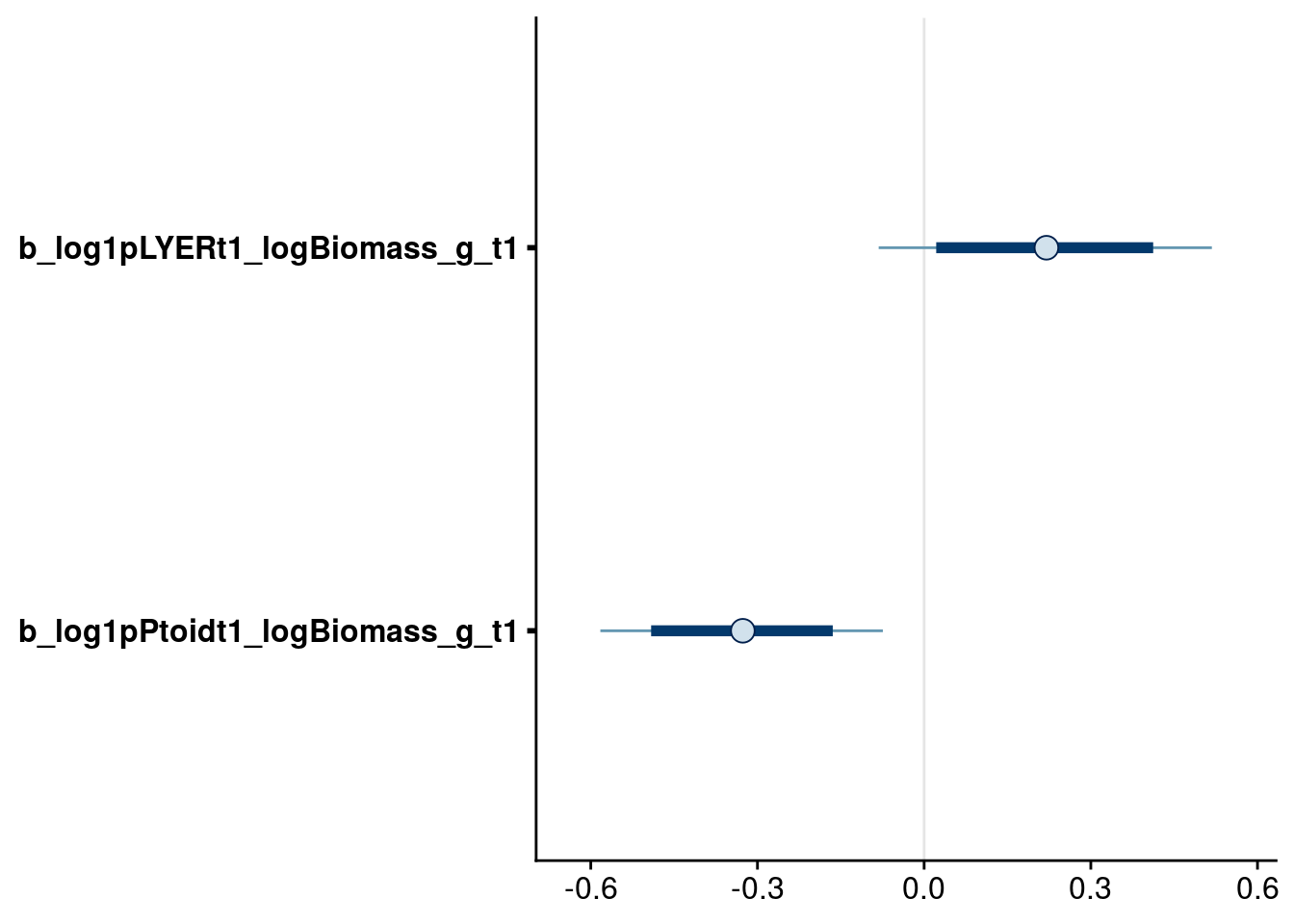

Past versions of reduced-8-summary-1.png

Version	Author	Date
86116c8	mabarbour	2020-06-23

Model comparison

# add leave-one-out (loo) cross-validation criterion to each model
full.mv.norm.brm <- add_criterion(full.mv.norm.brm, criterion = "loo", force_save = T, reloo = T)
# reduced.1.brm # intermediate model on way to determine 80% cutoff, I so don't use it for comparison
reduced.2.brm <- add_criterion(reduced.2.brm, criterion = "loo", force_save = T, reloo = T) 
reduced.3.brm <- add_criterion(reduced.3.brm, criterion = "loo", force_save = T, reloo = T) 
reduced.4.brm <- add_criterion(reduced.4.brm, criterion = "loo", force_save = T, reloo = T) 
reduced.5.brm <- add_criterion(reduced.5.brm, criterion = "loo", force_save = T, reloo = T)
reduced.6.brm <- add_criterion(reduced.6.brm, criterion = "loo", force_save = T, reloo = T) 
reduced.7.brm <- add_criterion(reduced.7.brm, criterion = "loo", force_save = T) # reloo not needed
reduced.8.brm <- add_criterion(reduced.8.brm, criterion = "loo", force_save = T, reloo = T) 

# compare models
loo_compare(full.mv.norm.brm, # full model
            #reduced.1.brm, # intermediate model on way to determine 80% cutoff
            reduced.2.brm, # all parameters have >80% of their posterior estimates different from zero
            reduced.3.brm, # drop log1p(LYER_t):rich on Ptoid from 80% PP cutoff model
            reduced.4.brm, # drop log1p(BRBR_t):rich on Ptoid from 80% PP cutoff model
            reduced.5.brm, # drop all rich effects on Ptoid from 80% PP cutoff model
            reduced.6.brm, # drop all rich effects on LYER from 80% PP cutoff model
            reduced.7.brm, # drop all rich effects from 80% PP cutoff model
            reduced.8.brm, # drop all rich and temp effects from 80% PP cutoff model
            criterion = "loo",
            model_names = c("Full","80% PP cutoff","Drop LYER:rich for Ptoid","Drop BRBR:rich for Ptoid","Drop all rich for Ptoid","Drop all rich for LYER","Drop all rich effects","Drop all rich and temp effects"))

                               elpd_diff se_diff
Drop all rich effects            0.0       0.0  
Drop all rich for LYER          -1.8       2.5  
Drop LYER:rich for Ptoid        -2.1       3.0  
80% PP cutoff                   -2.3       3.5  
Drop BRBR:rich for Ptoid        -2.8       2.4  
Drop all rich for Ptoid         -3.3       3.6  
Full                           -19.2       6.0  
Drop all rich and temp effects -64.0       9.9  

As you can see, there are several models that provide similar fits to data for the initial food web (i.e., the standard error of the model fit overlaps with the top model). Of these models, however, only reduced.3.brm (i.e., “Drop LYER:rich for Ptoid”) was able to reproduce our observed genotype-specific effects on critical transitions in the dominant food chain (see Genotypic effects). Therefore, I used reduced.3.brm to assess the Structural stability of dominant food chain and Structural stability of initial food web.

Structural stability of dominant food chain

# specify the model for subsequent analysis
rich_model <- reduced.3.brm

Reproduce Fig. 4

Since our observational data indicated clear effects of genetic diversity on the persistence of the LYER-Ptoid subcommunity, I restrict our subsequent analysis to this effect (i.e. no temperature).

Remember that I set rich = 1 as the zero point for this model. Therefore, the intercept in the model corresponds to when rich = 1, and the effect of rich corresponds to a unit increase in rich (i.e., rich = 2).

Note that I did not specify an effect of richness on the intra- or interspecific interactions in LYER or Ptoid. Therefore, the interaction matrix is the same for all levels of richness.

Also, I did this comparison at an imaginary midpoint of temperature, i.e. temp = 1.5. In this food chain, temperature only had a clear effect on the parasitoid’s intrinsic growth rate, so I only add the temperature effect here.

coef.rich <- fixef(rich_model)[,"Estimate"]

# value of rich to condition
temp.cond <- 1.5 # 1.5 = 21.5 C
# I chose 1.5 to condition on
# an imaginary average between temperature treatments
# note that setting it to zero, represents temp = 20 C

# interaction matrix for all levels of rich
rich1.mat <- matrix(c(coef.rich["log1pLYERt1_log1pLYER_t"], 
                      coef.rich["log1pLYERt1_log1pPtoid_t"],
                      coef.rich["log1pPtoidt1_log1pLYER_t"], 
                      0), # set to zero because there was no clear evidence for intraspecific Ptoid effect
                    ncol = 2, byrow = TRUE)
rich1.mat

           [,1]       [,2]
[1,] -0.5837297 -0.7150802
[2,]  0.3990346  0.0000000

rich2.mat <- rich1.mat
rich4.mat <- rich1.mat

# growth rates when rich = 1
rich1.IGR <- matrix(c(coef.rich["log1pLYERt1_intercept"],
                      coef.rich["log1pPtoidt1_intercept"] + coef.rich["log1pPtoidt1_temp"]*temp.cond),
                    ncol = 1)
rich1.IGR

          [,1]
[1,]  2.744906
[2,] -2.419228

# growth rates when rich = 2
rich2.IGR <- matrix(c(coef.rich["log1pLYERt1_intercept"] + coef.rich["log1pLYERt1_rich"],
                      coef.rich["log1pPtoidt1_intercept"] + coef.rich["log1pPtoidt1_rich"] + coef.rich["log1pPtoidt1_temp"]*temp.cond), 
                    ncol = 1)
rich2.IGR

          [,1]
[1,]  3.122174
[2,] -2.237049

# growth rates when rich = 4
rich4.IGR <- matrix(c(coef.rich["log1pLYERt1_intercept"] + coef.rich["log1pLYERt1_rich"]*3,
                      coef.rich["log1pPtoidt1_intercept"] + coef.rich["log1pPtoidt1_rich"]*3 + coef.rich["log1pPtoidt1_temp"]*temp.cond), 
                    ncol = 1)
rich4.IGR

          [,1]
[1,]  3.876709
[2,] -1.872689

Plot the effect of genetic diversity on structural stability.

# get raw data for manually making plot
get_FD.2sp <- FeasibilityDomain2sp(A = list(rich1.mat, rich2.mat, rich4.mat),
                     r = list(rich1.IGR, rich2.IGR, rich4.IGR),
                     labels = c("1", "2", "4"),
                     normalize = TRUE) %>%
  rename(rich = A_ID) 

# Draw polygon for feasibility domain
# from: https://stackoverflow.com/questions/12794596/how-fill-part-of-a-circle-using-ggplot2
# define the circle; add a point at the center if the 'pie slice' if the shape is to be filled
circleFun <- function(center=c(0,0), diameter=1, npoints=100, start=0, end=2, filled=TRUE){
  tt <- seq(start*pi, end*pi, length.out=npoints)
  df <- data.frame(
    x = center[1] + diameter / 2 * cos(tt),
    y = center[2] + diameter / 2 * sin(tt)
  )
  if(filled==TRUE) { #add a point at the center so the whole 'pie slice' is filled
    df <- rbind(df, center)
  }
  return(df)
}

# new version
ggplot(filter(get_FD.2sp, Type == "r"), aes(x = Sp_1, y = Sp_2, size = rich)) +
  # draw intrinsic growth rate vectors
  geom_segment(aes(x = 0, y = 0, xend = Sp_1, yend = Sp_2),
               arrow = arrow(length = unit(0.3,"cm"))) +
  # draw critical boundary
  #geom_segment(data = filter(get_FD.2sp, Type == "A")[1,], # just need one lower bound
  #             aes(x = 0, y = 0, xend = Sp_1, yend = Sp_2, linetype = "Critical\nboundary"),
  #             color = "black",
  #             size = 0.5) + 
  #scale_linetype_manual(values = "dotted", name = "") +
  xlab("Aphid growth rate (normalized)") + 
  ylab("Parasitoid growth rate (normalized)") +
  # illustrate circular nature of feasibility domain
  coord_cartesian(xlim = c(0,1), ylim = c(0.0,-0.75), expand = F) + 
  scale_size_manual(values = c(0.25,0.5,1), labels = c("1 genotype","2 genotypes","4 genotypes"), name = "") +
  # adjusted until critical boundary was correct
  geom_polygon(data=circleFun(c(0,0), diameter = 2, start=0, end=-0.191, npoints=100, filled=TRUE), 
               aes(x,y), alpha = 0.1, inherit.aes = F) +
  theme_cowplot(font_size = 18, line_size = 1)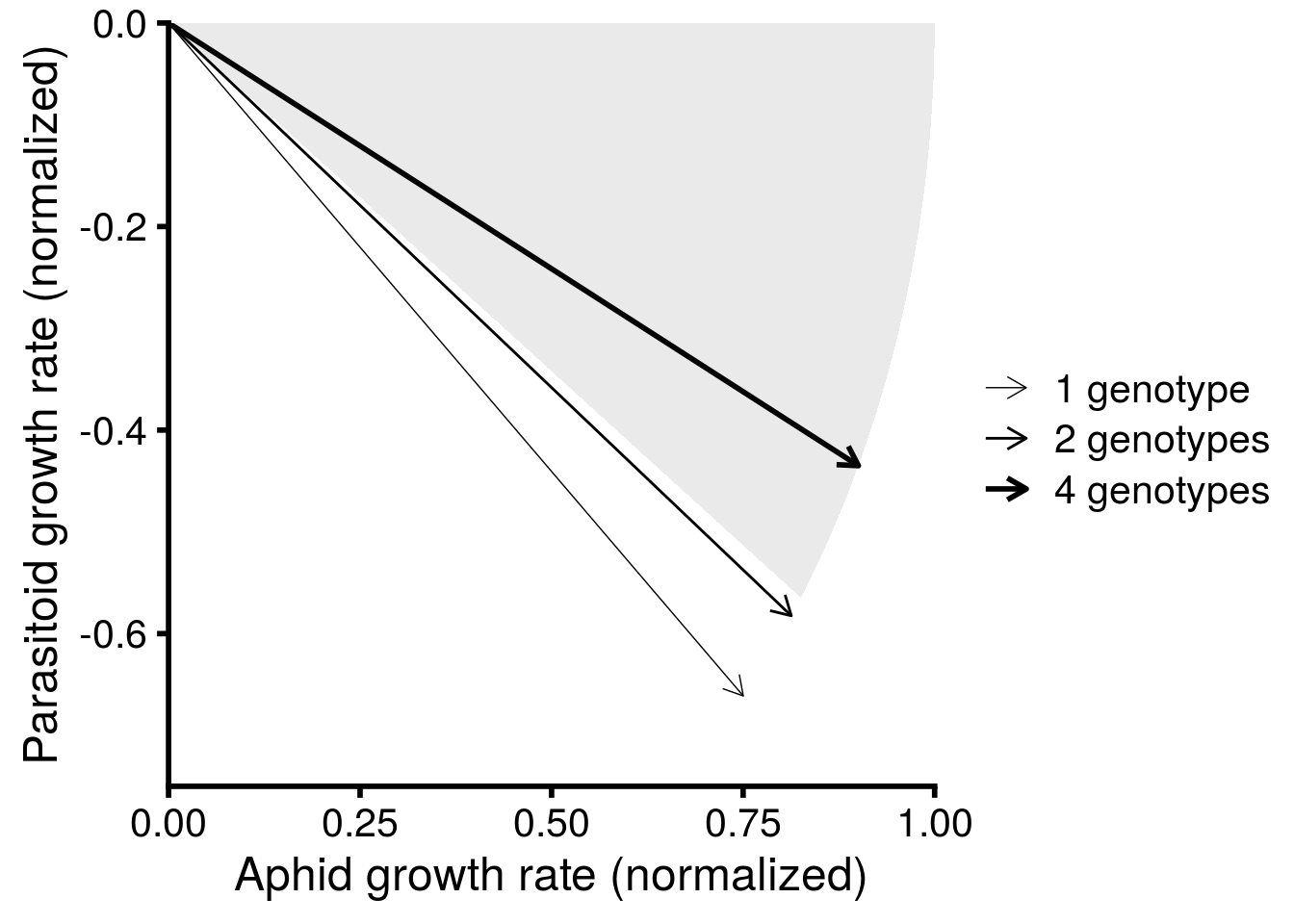

Past versions of rich-feasibility-domain-1.png

Version	Author	Date
86116c8	mabarbour	2020-06-23

ggsave("figures/rich-structural-stability-R-v2.pdf", width = 8, height = 8, units = "in") 

I then used Keynote to manually add images and text to create the final version presented in Figure 4 of the main text.

And just as a quick check, the above plot suggests that the community is only feasible (all three species have positive abundances at equilibrium) when there are 4 genotypes, which is true:

-inv(rich1.mat)%*%rich1.IGR # Ptoid goes extinct

          [,1]
[1,]  6.062704
[2,] -1.110468

-inv(rich2.mat)%*%rich2.IGR # Ptoid goes extinct

           [,1]
[1,]  5.6061526
[2,] -0.2101917

-inv(rich4.mat)%*%rich4.IGR # Coexistence

         [,1]
[1,] 4.693051
[2,] 1.590362

Non-equilibrium simulation (Fig. S6)

The above plot illustrates the effect of genetic diversity on the structural stability of the equilibrium abundances of species. I can explore whether our results hold in a non-equilibrium scenario that better characterizes our observational data.

To do this, I look at the the effect of genetic diversity across a range of initial conditions for the abundances of LYER and Ptoid. I get this data by simulating community dynamics with the observed effects of genetic diversity across a range of intial conditions. I restricted our simulation to 10 time steps, as BRBR went extinct commonly at week 7 (experiment was 17 weeks long). I also set an extinction threshold of log(abundance) = 1.

LP_duration <- 10
LP_threshold <- 1 
res <- 0.1
LP_test_df <- expand.grid(LYER = seq(1, 6, by = res), Ptoid = seq(1, 6, by = res))

## simulate population dynamics and determine which species goes extinct

# rich = 1
FE_LP_rich1 <- list()
for(i in 1:length(LP_test_df$LYER)){
  FE_LP_rich1[[i]] <- first_extinction_2sp(Initial.States = c(LYER = LP_test_df[i,"LYER"], Ptoid = LP_test_df[i,"Ptoid"]), 
                                          Interaction.Matrix = rich1.mat + diag(2), 
                                          IGR.Vector = rich1.IGR, 
                                          Duration = LP_duration, 
                                          threshold = LP_threshold)
}
FE_LP_rich1_df <- bind_cols(LP_test_df, plyr::ldply(FE_LP_rich1)) %>%
  mutate(rich = 1)

# rich = 2
FE_LP_rich2 <- list()
for(i in 1:length(LP_test_df$LYER)){
  FE_LP_rich2[[i]] <- first_extinction_2sp(Initial.States = c(LYER = LP_test_df[i,"LYER"], Ptoid = LP_test_df[i,"Ptoid"]), 
                                           Interaction.Matrix = rich2.mat + diag(2), 
                                           IGR.Vector = rich2.IGR, 
                                           Duration = LP_duration, 
                                           threshold = LP_threshold)
}
FE_LP_rich2_df <- bind_cols(LP_test_df, plyr::ldply(FE_LP_rich2)) %>%
  mutate(rich = 2)

# rich = 4
FE_LP_rich4 <- list()
for(i in 1:length(LP_test_df$LYER)){
  FE_LP_rich4[[i]] <- first_extinction_2sp(Initial.States = c(LYER = LP_test_df[i,"LYER"], Ptoid = LP_test_df[i,"Ptoid"]), 
                                           Interaction.Matrix = rich4.mat + diag(2), 
                                           IGR.Vector = rich4.IGR, 
                                           Duration = LP_duration, 
                                           threshold = LP_threshold)
}
FE_LP_rich4_df <- bind_cols(LP_test_df, plyr::ldply(FE_LP_rich4)) %>%
  mutate(rich = 4)

# get observed data on initial abundances of LYER and Ptoid after BRBR went extinct
LP_actual_df <- timeseries_df %>%
  filter(BRBR_t == 0, LYER_t > 0, Ptoid_t > 0) %>%
  group_by(rich, Cage) %>%
  summarise_at(vars(LYER_t, Ptoid_t), list(first = first)) %>%
  ungroup() %>%
  mutate(rich = rich + 1, 
         log1p_LYER_t_first = log1p(LYER_t_first),
         log1p_Ptoid_t_first = log1p(Ptoid_t_first)) %>%
  as.data.frame()

The graph below shows a couple of useful things. First, our predictions hold for outside of equilibrium. That is, there is a greater likelihood of LYER-Ptoid persistence with increasing genetic diversity. Note the threshold between rich = 2 and rich = 4. This likely reflects the fact that the equilibrium community was only feasible when rich = 4.

It’s also important to note that there is a region of parameter space where LYER goes extinct before Ptoid, which would eventually lead to the collapse of the Ptoid since it has lost its resource. This is not possible if I were to assume the community is at equilibrium. It also suggests that the likelihood of LYER going extinct before the Ptoid is more likely at lower levels of genetic diversity. I also observe this in our empirical data, as LYER going extinct before the Ptoid never occurred when rich = 4.

cbPalette <-  viridis::viridis(4)

bind_rows(FE_LP_rich1_df, FE_LP_rich2_df, FE_LP_rich4_df) %>%
  mutate(rich = factor(rich, labels = c("1 genotype","2 genotypes","4 genotypes"))) %>%
  mutate(species = ifelse(is.na(species) == T, "Food chain persists", species),
         fspecies = factor(species, levels = c("LYER","Ptoid","Food chain persists"), labels = c("Complete collapse","Aphid only","Food chain persists"))) %>%
  ggplot(., aes(x = LYER, y = Ptoid, fill = fspecies)) +
  geom_tile() +
  facet_grid(~rich) +
  scale_fill_manual(name = "Critical transition", values = cbPalette[1:3]) + 
  coord_cartesian(xlim = c(1, max(LP_actual_df$log1p_LYER_t_first)), 
                  ylim = c(1, max(LP_actual_df$log1p_Ptoid_t_first))) +
  xlab("Aphid initial abundance (log scale)") +
  ylab("Parasitoid initial abundance (log scale)") +
  theme(strip.background = element_blank())

Past versions of nonequilibrium-plot-1.png

Version	Author	Date
86116c8	mabarbour	2020-06-23

Remember though that our real communities are also stochastic, which is something I did not include in this non-equilibrium simulation. Below, I explicitly address stochasticity by estimating the uncertainty in our observed “mean” effects of genetic diversity on structural stability.

Posterior estimates (Fig. S5)

The above is a nice visualization of the central tendency, but it doesn’t illustrate the uncertainty in the effect of genetic richness on structural stability. To get at this, I need to use the posterior samples from our model.

# get posterior predictions
pp.rich_model <- posterior_samples(rich_model, pars = "^b")

# calculate structural stability when rich = 1
rich1_stability <- apply(
  pp.rich_model, 
  MARGIN = 1, 
  FUN = function(x) { 
    tmp.mat = matrix(c(x["b_log1pLYERt1_log1pLYER_t"], x["b_log1pLYERt1_log1pPtoid_t"],
                       x["b_log1pPtoidt1_log1pLYER_t"], 0), 
                     ncol = 2, byrow = TRUE)
    tmp.r = matrix(c(x["b_log1pLYERt1_intercept"],
                     x["b_log1pPtoidt1_intercept"] + x["b_log1pPtoidt1_temp"]*temp.cond),
                   ncol = 1)
    FeasibilityBoundaryLYER.Ptoid = as.numeric(BoundaryLYER.Ptoid(tmp.mat, tmp.r)["boundary"])
    c(FeasibilityBoundaryLYER.Ptoid = FeasibilityBoundaryLYER.Ptoid)
  })
rich1_stability.df <- data.frame(
  rich = 1,
  posterior_sample = 1:nrow(pp.rich_model),
  FeasibilityBoundaryLYER.Ptoid = rich1_stability
)

# calculate structural stability when rich = 2
rich2_stability <- apply(
  pp.rich_model, 
  MARGIN = 1, 
  FUN = function(x) { 
    tmp.mat = matrix(c(x["b_log1pLYERt1_log1pLYER_t"], x["b_log1pLYERt1_log1pPtoid_t"],
                       x["b_log1pPtoidt1_log1pLYER_t"], 0), 
                     ncol = 2, byrow = TRUE)
    tmp.r = matrix(c(x["b_log1pLYERt1_intercept"] + x["b_log1pLYERt1_rich"],
                     x["b_log1pPtoidt1_intercept"] +  x["b_log1pPtoidt1_rich"] + x["b_log1pPtoidt1_temp"]*temp.cond),  
                   ncol = 1)
    FeasibilityBoundaryLYER.Ptoid = as.numeric(BoundaryLYER.Ptoid(tmp.mat, tmp.r)["boundary"]) 
    c(FeasibilityBoundaryLYER.Ptoid = FeasibilityBoundaryLYER.Ptoid)
  })
rich2_stability.df <- data.frame(
  rich = 2,
  posterior_sample = 1:nrow(pp.rich_model),
  FeasibilityBoundaryLYER.Ptoid = rich2_stability
)

# calculate structural stability when rich = 4
rich4_stability <- apply(
  pp.rich_model, 
  MARGIN = 1, 
  FUN = function(x) { 
    tmp.mat = matrix(c(x["b_log1pLYERt1_log1pLYER_t"], x["b_log1pLYERt1_log1pPtoid_t"],
                       x["b_log1pPtoidt1_log1pLYER_t"], 0), 
                     ncol = 2, byrow = TRUE)
    tmp.r = matrix(c(x["b_log1pLYERt1_intercept"] + x["b_log1pLYERt1_rich"]*3,
                     x["b_log1pPtoidt1_intercept"] +  x["b_log1pPtoidt1_rich"]*3 + x["b_log1pPtoidt1_temp"]*temp.cond),  
                   ncol = 1)
    FeasibilityBoundaryLYER.Ptoid = as.numeric(BoundaryLYER.Ptoid(tmp.mat, tmp.r)["boundary"]) 
    c(FeasibilityBoundaryLYER.Ptoid = FeasibilityBoundaryLYER.Ptoid)
  })
rich4_stability.df <- data.frame(
  rich = 4,
  posterior_sample = 1:nrow(pp.rich_model),
  FeasibilityBoundaryLYER.Ptoid = rich4_stability
)

# combine data
all.rich_stability.df <- bind_rows(rich1_stability.df, rich2_stability.df, rich4_stability.df)

Reproduce Fig. S5

# subsample 1/8 of the posterior to make it easier to visualize
set.seed(38)
rsamp <- sample(1:8000, size = 1000)

# plot
all.rich_stability.df %>%
  filter(posterior_sample %in% rsamp) %>%
  ggplot(., aes(x = rich, y = FeasibilityBoundaryLYER.Ptoid)) +
  geom_line(aes(group = posterior_sample), alpha = 0.1) +
  stat_summary(fun.y = mean, geom = "line", color = "red") +
  theme_minimal_hgrid() +
  ylab("Normalized angle from critical boundary") +
  xlab("Genetic diversity (no. of genotypes)")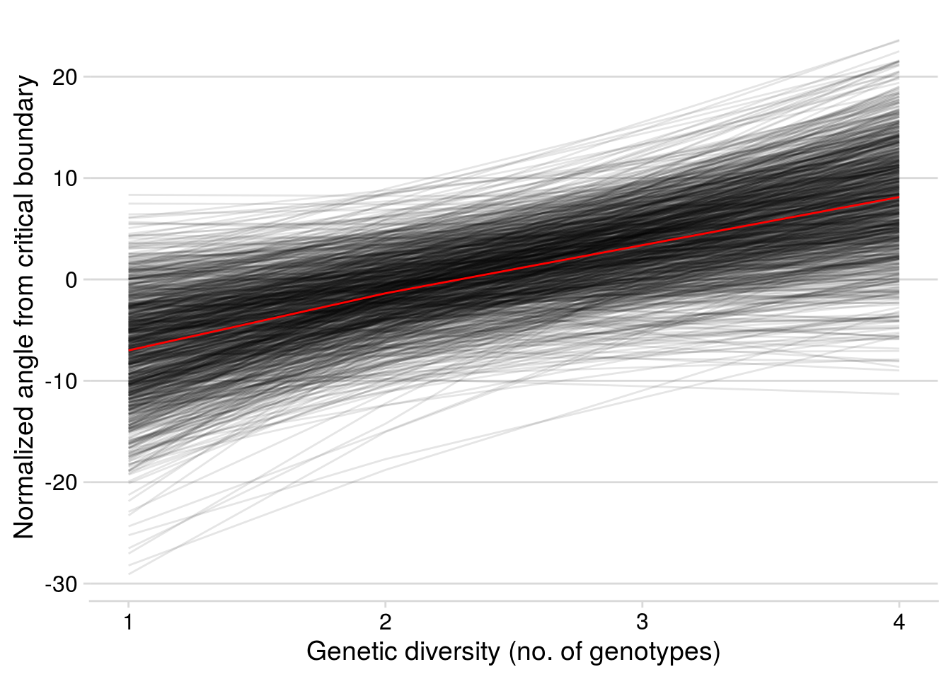

Past versions of unnamed-chunk-4-1.png

Version	Author	Date
86116c8	mabarbour	2020-06-23

Calculate the percentage of posterior estimates where genetic diversity increased the structural stability of the community.

# organize data
rich_LPbound <- all.rich_stability.df %>%
  select(rich, posterior_sample, FeasibilityBoundaryLYER.Ptoid) %>%
  spread(rich, FeasibilityBoundaryLYER.Ptoid) %>%
  mutate(rich_effect = `2` - `1`)

# calculate percentage
mean(rich_LPbound$rich_effect > 0)

[1] 0.97775

Genotypic effects

I first modify rich_model by replacing rich with (Col + gsm1 + AOP2 + AOP2.gsoh), which are the components of the rich effect.

## formulas
geno.rich_model.BRBR.bf <- reduced.3.BRBR.bf 
geno.rich_model.LYER.bf <- update(reduced.3.LYER.bf, .~. 
                                  -rich + (Col + gsm1 + AOP2 + AOP2.gsoh) 
                                  -log1p(BRBR_t):rich + log1p(BRBR_t):(Col + gsm1 + AOP2 + AOP2.gsoh))
geno.rich_model.Ptoid.bf <- update(reduced.3.Ptoid.bf, .~. 
                                  -rich + (Col + gsm1 + AOP2 + AOP2.gsoh) 
                                  -log1p(BRBR_t):rich + log1p(BRBR_t):(Col + gsm1 + AOP2 + AOP2.gsoh))

## fit new model
geno.rich_model.brm <- brm(
  data = full_df,
  mvbf(geno.rich_model.BRBR.bf, geno.rich_model.LYER.bf, geno.rich_model.Ptoid.bf),
  iter = 4000,
  prior = c(# growth rates
            set_prior(prior.r.BRBR, class = "b", coef = "intercept", resp = "log1pBRBRt1"),
            set_prior(prior.r.LYER, class = "b", coef = "intercept", resp = "log1pLYERt1"),
            set_prior(prior.r.Ptoid, class = "b", coef = "intercept", resp = "log1pPtoidt1"),
            # intraspecific effects
            set_prior(prior.intra.BRBR, class = "b", coef = "log1pBRBR_t", resp = "log1pBRBRt1"),
            set_prior(prior.intra.LYER, class = "b", coef = "log1pLYER_t", resp = "log1pLYERt1"),
            # negative interspecific effects
            set_prior(prior.BRBRonLYER, class = "b", coef = "log1pBRBR_t", resp = "log1pLYERt1"),
            set_prior(prior.PtoidonBRBR, class = "b", coef = "log1pPtoid_t", resp = "log1pBRBRt1"),
            set_prior(prior.PtoidonLYER, class = "b", coef = "log1pPtoid_t", resp = "log1pLYERt1"),
            # positive interspecific effects
            set_prior(prior.BRBRonPtoid, class = "b", coef = "log1pBRBR_t", resp = "log1pPtoidt1"),
            set_prior(prior.LYERonPtoid, class = "b", coef = "log1pLYER_t", resp = "log1pPtoidt1"),
            # rich effects
            set_prior(prior.rich, class = "b", coef = "Col", resp = "log1pLYERt1"),
            set_prior(prior.rich, class = "b", coef = "log1pBRBR_t:Col", resp = "log1pLYERt1"),
            set_prior(prior.rich, class = "b", coef = "gsm1", resp = "log1pLYERt1"),
            set_prior(prior.rich, class = "b", coef = "log1pBRBR_t:gsm1", resp = "log1pLYERt1"),
            set_prior(prior.rich, class = "b", coef = "AOP2", resp = "log1pLYERt1"),
            set_prior(prior.rich, class = "b", coef = "log1pBRBR_t:AOP2", resp = "log1pLYERt1"),
            set_prior(prior.rich, class = "b", coef = "AOP2.gsoh", resp = "log1pLYERt1"),
            set_prior(prior.rich, class = "b", coef = "log1pBRBR_t:AOP2.gsoh", resp = "log1pLYERt1"),
            set_prior(prior.rich, class = "b", coef = "Col", resp = "log1pPtoidt1"),
            set_prior(prior.rich, class = "b", coef = "log1pBRBR_t:Col", resp = "log1pPtoidt1"),
            set_prior(prior.rich, class = "b", coef = "gsm1", resp = "log1pPtoidt1"),
            set_prior(prior.rich, class = "b", coef = "log1pBRBR_t:gsm1", resp = "log1pPtoidt1"),
            set_prior(prior.rich, class = "b", coef = "AOP2", resp = "log1pPtoidt1"),
            set_prior(prior.rich, class = "b", coef = "log1pBRBR_t:AOP2", resp = "log1pPtoidt1"),
            set_prior(prior.rich, class = "b", coef = "AOP2.gsoh", resp = "log1pPtoidt1"),
            set_prior(prior.rich, class = "b", coef = "log1pBRBR_t:AOP2.gsoh", resp = "log1pPtoidt1"),
            # temp effects
            set_prior(prior.temp, class = "b", coef = "temp", resp = "log1pBRBRt1"),
            set_prior(prior.temp, class = "b", coef = "temp", resp = "log1pPtoidt1"),  
            set_prior(prior.temp, class = "b", coef = "log1pBRBR_t:temp", resp = "log1pBRBRt1"),
            set_prior(prior.temp, class = "b", coef = "log1pBRBR_t:temp", resp = "log1pPtoidt1"),
            set_prior(prior.temp, class = "b", coef = "log1pPtoid_t:temp", resp = "log1pBRBRt1"),
            # biomass effects
            set_prior(prior.AphidBiomass, class = "b", coef = "logBiomass_g_t1", resp = "log1pLYERt1"),
            set_prior(prior.PtoidBiomass, class = "b", coef = "logBiomass_g_t1", resp = "log1pPtoidt1"),
            # random effects
            set_prior(prior.random.effects, class = "sd", resp = "log1pBRBRt1"),
            set_prior(prior.random.effects, class = "sd", resp = "log1pLYERt1"),
            set_prior(prior.random.effects, class = "sd", resp = "log1pPtoidt1")),
  file = "output/geno.rich_model.brm.rds") 

# print summary
summary(geno.rich_model.brm)

 Family: MV(gaussian, gaussian, gaussian) 
  Links: mu = identity; sigma = identity
         mu = identity; sigma = identity
         mu = identity; sigma = identity 
Formula: log1p(BRBR_t1) ~ intercept + log1p(BRBR_t) + log1p(Ptoid_t) + temp + (1 | Cage) + ar(time = Week_match.1p, gr = Cage, p = 1, cov = FALSE) + log1p(BRBR_t):temp + log1p(Ptoid_t):temp + offset(log1p(BRBR_t)) - 1 
         log1p(LYER_t1) ~ intercept + log1p(BRBR_t) + log1p(LYER_t) + log1p(Ptoid_t) + log(Biomass_g_t1) + (1 | Cage) + ar(time = Week_match.1p, gr = Cage, p = 1, cov = FALSE) + Col + gsm1 + AOP2 + AOP2.gsoh + log1p(BRBR_t):Col + log1p(BRBR_t):gsm1 + log1p(BRBR_t):AOP2 + log1p(BRBR_t):AOP2.gsoh + offset(log1p(LYER_t)) - 1 
         log1p(Ptoid_t1) ~ intercept + log1p(BRBR_t) + log1p(LYER_t) + temp + log(Biomass_g_t1) + (1 | Cage) + ar(time = Week_match.1p, gr = Cage, p = 1, cov = FALSE) + Col + gsm1 + AOP2 + AOP2.gsoh + log1p(BRBR_t):temp + log1p(BRBR_t):Col + log1p(BRBR_t):gsm1 + log1p(BRBR_t):AOP2 + log1p(BRBR_t):AOP2.gsoh + offset(log1p(Ptoid_t)) - 1 
   Data: full_df (Number of observations: 264) 
Samples: 4 chains, each with iter = 4000; warmup = 2000; thin = 1;
         total post-warmup samples = 8000

Correlation Structures:
                   Estimate Est.Error l-95% CI u-95% CI Rhat Bulk_ESS Tail_ESS
ar_log1pBRBRt1[1]     -0.45      0.09    -0.63    -0.26 1.00     3923     5401
ar_log1pLYERt1[1]     -0.11      0.10    -0.29     0.09 1.00     4849     5799
ar_log1pPtoidt1[1]    -0.49      0.08    -0.65    -0.33 1.00    10963     6664

Group-Level Effects: 
~Cage (Number of levels: 60) 
                           Estimate Est.Error l-95% CI u-95% CI Rhat Bulk_ESS
sd(log1pBRBRt1_Intercept)      0.26      0.10     0.04     0.44 1.01     1281
sd(log1pLYERt1_Intercept)      0.14      0.09     0.01     0.32 1.00     1850
sd(log1pPtoidt1_Intercept)     0.04      0.03     0.00     0.11 1.00     5278
                           Tail_ESS
sd(log1pBRBRt1_Intercept)      1390
sd(log1pLYERt1_Intercept)      3358
sd(log1pPtoidt1_Intercept)     4207

Population-Level Effects: 
                                   Estimate Est.Error l-95% CI u-95% CI Rhat
log1pBRBRt1_intercept                  1.46      0.45     0.59     2.35 1.00
log1pBRBRt1_log1pBRBR_t                0.04      0.07    -0.11     0.18 1.00
log1pBRBRt1_log1pPtoid_t              -0.90      0.05    -1.00    -0.80 1.00
log1pBRBRt1_temp                      -0.30      0.22    -0.72     0.12 1.00
log1pBRBRt1_log1pBRBR_t:temp          -0.07      0.04    -0.14    -0.00 1.00
log1pBRBRt1_log1pPtoid_t:temp          0.13      0.04     0.06     0.20 1.00
log1pLYERt1_intercept                  3.07      0.59     1.88     4.27 1.00
log1pLYERt1_log1pBRBR_t                0.31      0.09     0.14     0.48 1.00
log1pLYERt1_log1pLYER_t               -0.65      0.09    -0.83    -0.48 1.00
log1pLYERt1_log1pPtoid_t              -0.73      0.05    -0.83    -0.63 1.00
log1pLYERt1_logBiomass_g_t1            0.08      0.18    -0.27     0.44 1.00
log1pLYERt1_Col                        0.37      0.31    -0.24     0.98 1.00
log1pLYERt1_gsm1                       0.26      0.31    -0.35     0.85 1.00
log1pLYERt1_AOP2                       0.03      0.31    -0.58     0.64 1.00
log1pLYERt1_AOP2.gsoh                  0.40      0.31    -0.20     0.99 1.00
log1pLYERt1_log1pBRBR_t:Col           -0.03      0.07    -0.16     0.09 1.00
log1pLYERt1_log1pBRBR_t:gsm1          -0.03      0.07    -0.16     0.10 1.00
log1pLYERt1_log1pBRBR_t:AOP2          -0.02      0.07    -0.15     0.11 1.00
log1pLYERt1_log1pBRBR_t:AOP2.gsoh     -0.11      0.07    -0.24     0.02 1.00
log1pPtoidt1_intercept                -3.11      0.45    -3.98    -2.23 1.00
log1pPtoidt1_log1pBRBR_t               0.40      0.09     0.23     0.57 1.00
log1pPtoidt1_log1pLYER_t               0.35      0.07     0.22     0.47 1.00
log1pPtoidt1_temp                      0.65      0.12     0.42     0.89 1.00
log1pPtoidt1_logBiomass_g_t1          -0.69      0.17    -1.03    -0.35 1.00
log1pPtoidt1_Col                       0.25      0.26    -0.27     0.76 1.00
log1pPtoidt1_gsm1                      0.37      0.27    -0.17     0.90 1.00
log1pPtoidt1_AOP2                     -0.08      0.27    -0.60     0.45 1.00
log1pPtoidt1_AOP2.gsoh                -0.09      0.26    -0.62     0.42 1.00
log1pPtoidt1_log1pBRBR_t:temp         -0.16      0.02    -0.21    -0.12 1.00
log1pPtoidt1_log1pBRBR_t:Col          -0.04      0.06    -0.15     0.07 1.00
log1pPtoidt1_log1pBRBR_t:gsm1         -0.05      0.06    -0.16     0.06 1.00
log1pPtoidt1_log1pBRBR_t:AOP2         -0.00      0.06    -0.11     0.11 1.00
log1pPtoidt1_log1pBRBR_t:AOP2.gsoh     0.00      0.06    -0.11     0.11 1.00
                                   Bulk_ESS Tail_ESS
log1pBRBRt1_intercept                  3724     4984
log1pBRBRt1_log1pBRBR_t                4418     5634
log1pBRBRt1_log1pPtoid_t               4714     5542
log1pBRBRt1_temp                       4335     5259
log1pBRBRt1_log1pBRBR_t:temp           4672     5686
log1pBRBRt1_log1pPtoid_t:temp          6553     6331
log1pLYERt1_intercept                  4620     5364
log1pLYERt1_log1pBRBR_t                5168     5142
log1pLYERt1_log1pLYER_t                4768     6014
log1pLYERt1_log1pPtoid_t               5903     6396
log1pLYERt1_logBiomass_g_t1            9638     6338
log1pLYERt1_Col                        6748     6225
log1pLYERt1_gsm1                       6627     5751
log1pLYERt1_AOP2                       6444     5962
log1pLYERt1_AOP2.gsoh                  6522     5999
log1pLYERt1_log1pBRBR_t:Col            6878     5683
log1pLYERt1_log1pBRBR_t:gsm1           6418     6253
log1pLYERt1_log1pBRBR_t:AOP2           6490     5787
log1pLYERt1_log1pBRBR_t:AOP2.gsoh      6460     5579
log1pPtoidt1_intercept                 5157     5723
log1pPtoidt1_log1pBRBR_t               4762     5676
log1pPtoidt1_log1pLYER_t               9179     5794
log1pPtoidt1_temp                      6193     5885
log1pPtoidt1_logBiomass_g_t1           9417     6608
log1pPtoidt1_Col                       6463     6296
log1pPtoidt1_gsm1                      6713     6047
log1pPtoidt1_AOP2                      7189     5968
log1pPtoidt1_AOP2.gsoh                 6689     5908
log1pPtoidt1_log1pBRBR_t:temp          6394     5833
log1pPtoidt1_log1pBRBR_t:Col           6303     5942
log1pPtoidt1_log1pBRBR_t:gsm1          6666     5749
log1pPtoidt1_log1pBRBR_t:AOP2          7457     6175
log1pPtoidt1_log1pBRBR_t:AOP2.gsoh     6615     5715

Family Specific Parameters: 
                   Estimate Est.Error l-95% CI u-95% CI Rhat Bulk_ESS Tail_ESS
sigma_log1pBRBRt1      1.11      0.06     1.00     1.23 1.00     3767     5221
sigma_log1pLYERt1      0.92      0.04     0.84     1.01 1.00     8728     5993
sigma_log1pPtoidt1     0.76      0.03     0.70     0.83 1.00    14675     5618

Residual Correlations: 
                                 Estimate Est.Error l-95% CI u-95% CI Rhat
rescor(log1pBRBRt1,log1pLYERt1)      0.52      0.05     0.42     0.61 1.00
rescor(log1pBRBRt1,log1pPtoidt1)    -0.04      0.07    -0.18     0.10 1.00
rescor(log1pLYERt1,log1pPtoidt1)     0.06      0.07    -0.08     0.19 1.00
                                 Bulk_ESS Tail_ESS
rescor(log1pBRBRt1,log1pLYERt1)      8262     6288
rescor(log1pBRBRt1,log1pPtoidt1)     9931     6720
rescor(log1pLYERt1,log1pPtoidt1)    12325     6163

Samples were drawn using sampling(NUTS). For each parameter, Bulk_ESS
and Tail_ESS are effective sample size measures, and Rhat is the potential
scale reduction factor on split chains (at convergence, Rhat = 1).

Posterior estimates

# get posterior predictions
pp.geno.rich_model.norm <- posterior_samples(geno.rich_model.brm, pars = "^b")

# intercept term corresponds to a hypothetical plant population where each genotype is absent
int.mv_stability <- apply(
  pp.geno.rich_model.norm, 
  MARGIN = 1, 
  FUN = function(x) { 
    tmp.mat = matrix(c(x["b_log1pLYERt1_log1pLYER_t"], x["b_log1pLYERt1_log1pPtoid_t"],
                       x["b_log1pPtoidt1_log1pLYER_t"], 0), 
                     ncol = 2, byrow = TRUE)
    tmp.r = matrix(c(x["b_log1pLYERt1_intercept"],
                     x["b_log1pPtoidt1_intercept"] + x["b_log1pPtoidt1_temp"]*temp.cond),
                   ncol = 1)
    FeasibilityBoundaryLYER.Ptoid = as.numeric(BoundaryLYER.Ptoid(tmp.mat, tmp.r)["boundary"]) 
    c(FeasibilityBoundaryLYER.Ptoid = FeasibilityBoundaryLYER.Ptoid)
  })
int.mv_stability.df <- data.frame(
  geno = "int",
  posterior_sample = 1:nrow(pp.geno.rich_model.norm),
  FeasibilityBoundaryLYER.Ptoid = int.mv_stability
)


# Col effect on structural stability
Col.mv_stability <- apply(
  pp.geno.rich_model.norm, 
  MARGIN = 1, 
  FUN = function(x) { 
    tmp.mat = matrix(c(x["b_log1pLYERt1_log1pLYER_t"], x["b_log1pLYERt1_log1pPtoid_t"],
                       x["b_log1pPtoidt1_log1pLYER_t"], 0),
                     ncol = 2, byrow = TRUE)
    tmp.r = matrix(c(x["b_log1pLYERt1_intercept"] + x["b_log1pLYERt1_Col"],
                     x["b_log1pPtoidt1_intercept"] + x["b_log1pPtoidt1_Col"] + x["b_log1pPtoidt1_temp"]*temp.cond),
                   ncol = 1)
    FeasibilityBoundaryLYER.Ptoid = as.numeric(BoundaryLYER.Ptoid(tmp.mat, tmp.r)["boundary"]) 
    c(FeasibilityBoundaryLYER.Ptoid = FeasibilityBoundaryLYER.Ptoid)
  })
Col.mv_stability.df <- data.frame(
  geno = "Col",
  posterior_sample = 1:nrow(pp.geno.rich_model.norm),
  FeasibilityBoundaryLYER.Ptoid = Col.mv_stability
)

# gsm1 effect on structural stability
gsm1.mv_stability <- apply(
  pp.geno.rich_model.norm, 
  MARGIN = 1, 
  FUN = function(x) { 
    tmp.mat = matrix(c(x["b_log1pLYERt1_log1pLYER_t"], x["b_log1pLYERt1_log1pPtoid_t"],
                       x["b_log1pPtoidt1_log1pLYER_t"], 0),
                     ncol = 2, byrow = TRUE)
    tmp.r = matrix(c(x["b_log1pLYERt1_intercept"] + x["b_log1pLYERt1_gsm1"],
                     x["b_log1pPtoidt1_intercept"] + x["b_log1pPtoidt1_gsm1"] + x["b_log1pPtoidt1_temp"]*temp.cond),
                   ncol = 1)
    FeasibilityBoundaryLYER.Ptoid = as.numeric(BoundaryLYER.Ptoid(tmp.mat, tmp.r)["boundary"]) 
    c(FeasibilityBoundaryLYER.Ptoid = FeasibilityBoundaryLYER.Ptoid)
  })
gsm1.mv_stability.df <- data.frame(
  geno = "gsm1",
  posterior_sample = 1:nrow(pp.geno.rich_model.norm),
  FeasibilityBoundaryLYER.Ptoid = gsm1.mv_stability
)

# AOP2 effect on structural stability
AOP2.mv_stability <- apply(
  pp.geno.rich_model.norm, 
  MARGIN = 1, 
  FUN = function(x) { 
    tmp.mat = matrix(c(x["b_log1pLYERt1_log1pLYER_t"], x["b_log1pLYERt1_log1pPtoid_t"],
                       x["b_log1pPtoidt1_log1pLYER_t"], 0),
                     ncol = 2, byrow = TRUE)
    tmp.r = matrix(c(x["b_log1pLYERt1_intercept"] + x["b_log1pLYERt1_AOP2"],
                     x["b_log1pPtoidt1_intercept"] + x["b_log1pPtoidt1_AOP2"] + x["b_log1pPtoidt1_temp"]*temp.cond),
                   ncol = 1)
    FeasibilityBoundaryLYER.Ptoid = as.numeric(BoundaryLYER.Ptoid(tmp.mat, tmp.r)["boundary"]) 
    c(FeasibilityBoundaryLYER.Ptoid = FeasibilityBoundaryLYER.Ptoid)
  })
AOP2.mv_stability.df <- data.frame(
  geno = "AOP2",
  posterior_sample = 1:nrow(pp.geno.rich_model.norm),
  FeasibilityBoundaryLYER.Ptoid = AOP2.mv_stability
)

# AOP2/gsoh effect on structural stability
AOP2.gsoh.mv_stability <- apply(
  pp.geno.rich_model.norm, 
  MARGIN = 1, 
  FUN = function(x) { 
    tmp.mat = matrix(c(x["b_log1pLYERt1_log1pLYER_t"], x["b_log1pLYERt1_log1pPtoid_t"],
                       x["b_log1pPtoidt1_log1pLYER_t"], 0),
                     ncol = 2, byrow = TRUE)
    tmp.r = matrix(c(x["b_log1pLYERt1_intercept"] + x["b_log1pLYERt1_AOP2.gsoh"],
                     x["b_log1pPtoidt1_intercept"] + x["b_log1pPtoidt1_AOP2.gsoh"] + x["b_log1pPtoidt1_temp"]*temp.cond),
                   ncol = 1)
    FeasibilityBoundaryLYER.Ptoid = as.numeric(BoundaryLYER.Ptoid((tmp.mat), tmp.r)["boundary"])
    c(FeasibilityBoundaryLYER.Ptoid = FeasibilityBoundaryLYER.Ptoid)
  })
AOP2.gsoh.mv_stability.df <- data.frame(
  geno = "AOP2.gsoh",
  posterior_sample = 1:nrow(pp.geno.rich_model.norm),
  FeasibilityBoundaryLYER.Ptoid = AOP2.gsoh.mv_stability
)

# combine data
all.geno.mv_stability.df <- bind_rows(
  int.mv_stability.df, 
  Col.mv_stability.df, 
  gsm1.mv_stability.df, 
  AOP2.mv_stability.df, 
  AOP2.gsoh.mv_stability.df)

Reproduce Fig. S7

Col_df <- bind_rows(int.mv_stability.df, Col.mv_stability.df) %>% mutate(compare = "Col", geno = ifelse(geno == "int", 0, 1))
gsm1_df <- bind_rows(int.mv_stability.df, gsm1.mv_stability.df) %>% mutate(compare = "gsm1", geno = ifelse(geno == "int", 0, 1))
AOP2_df <- bind_rows(int.mv_stability.df, AOP2.mv_stability.df) %>% mutate(compare = "AOP2", geno = ifelse(geno == "int", 0, 1))
AOP2.gsoh_df <- bind_rows(int.mv_stability.df, AOP2.gsoh.mv_stability.df) %>% mutate(compare = "AOP2.gsoh", geno = ifelse(geno == "int", 0, 1))

bind_rows(Col_df, gsm1_df, AOP2_df, AOP2.gsoh_df) %>%
  filter(posterior_sample %in% rsamp) %>%
  mutate(compare = factor(compare, levels = c("Col","gsm1","AOP2","AOP2.gsoh"), labels = c("Col-0","gsm1","AOP2","AOP2/gsoh"))) %>%
  ggplot(., aes(x = geno, y = FeasibilityBoundaryLYER.Ptoid, color = compare)) +
  geom_line(aes(group = posterior_sample), alpha = 0.05) +
  stat_summary(fun.y = mean, geom = "line", size = 1.5) +
  facet_wrap(~compare, nrow = 1) +
  geom_hline(yintercept = 0, linetype = 'dotted') +
  ylab("Normalized angle from feasibility boundary") +
  scale_x_continuous(expand = c(0.1, 0.1), name = "", breaks = c(0,1), labels = c("Absent", "Present")) +
  scale_color_manual(values = c("darkgreen","steelblue","darkorange","firebrick1")) +
  theme_minimal_hgrid(font_size = 11) +
  theme(legend.position = "none")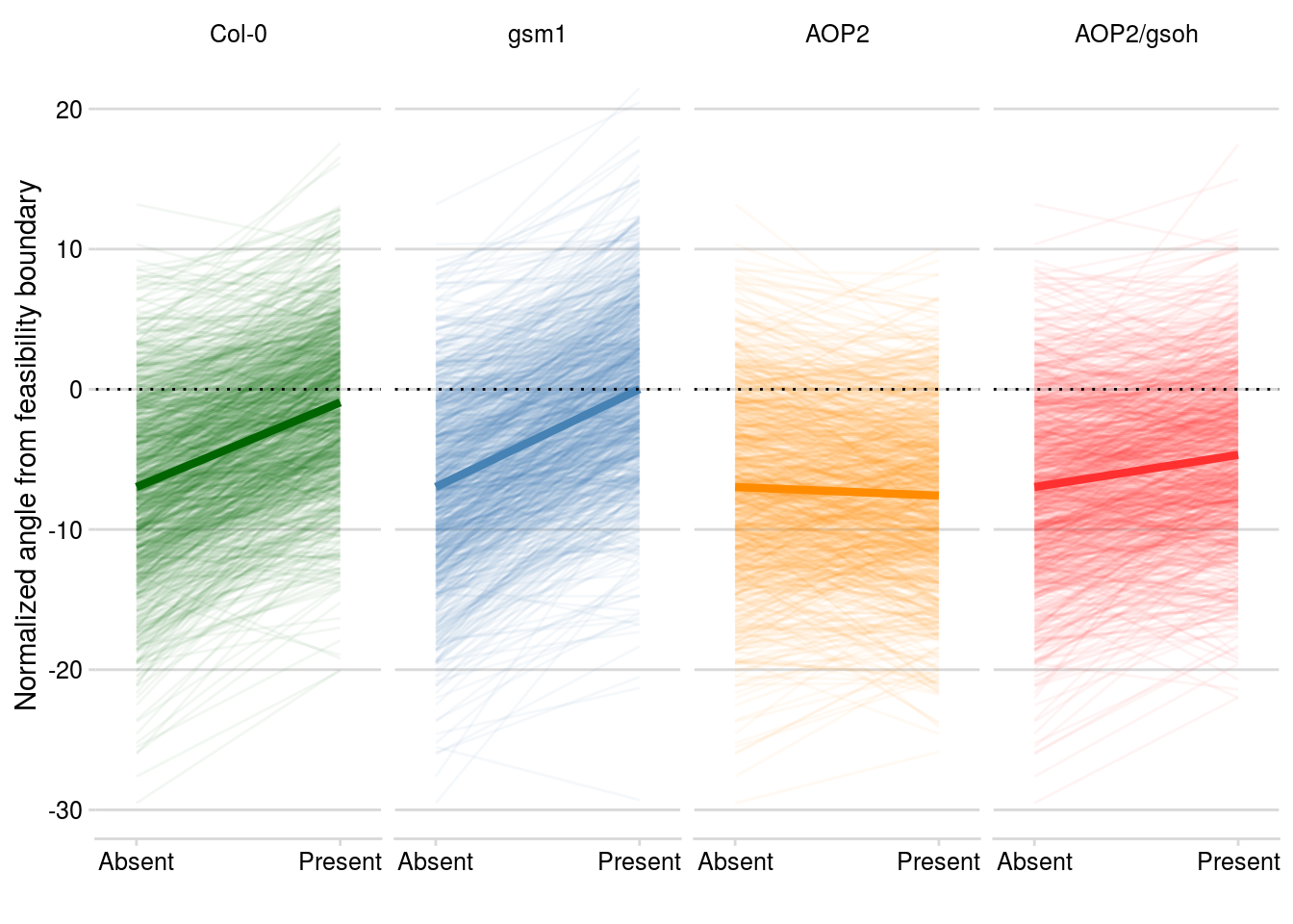

Past versions of plot-geno-structural-stability-1.png

Version	Author	Date
86116c8	mabarbour	2020-06-23

I then calculate the percentage of posterior samples where each genotype increases the structural stability of the community.

# gather data to calculate genotype-specific effects
geno_LPbound <- all.geno.mv_stability.df %>%
  select(geno, posterior_sample, FeasibilityBoundaryLYER.Ptoid) %>%
  spread(geno, FeasibilityBoundaryLYER.Ptoid) %>%
  mutate(Col_effect = (Col - int),
         gsm1_effect = (gsm1 - int),
         AOP2_effect = (AOP2 - int),
         AOP2.gsoh_effect = (AOP2.gsoh - int))

# effect of Col
mean(geno_LPbound$Col_effect > 0)

[1] 0.924125

# effect of gsm1
mean(geno_LPbound$gsm1_effect > 0)

[1] 0.937125

# effect of AOP2
mean(geno_LPbound$AOP2_effect > 0)

[1] 0.432375

# effect of AOP2/gsoh
mean(geno_LPbound$AOP2.gsoh_effect > 0)

[1] 0.695125

Structural stability of initial food web

I use the same model as I did for the effect of genetic diversity rich_model. Note that there were other models that did as good of, if not better, a job at predicting the dynamics of the initial food web. However, it was only reduced.3.brm (now rich_model) that could also reproduce the genotype-specific effects (see @ref{genotype-effects}).

temp_model <- rich_model

Reproduce Fig. S1

coef.temp <- fixef(temp_model)[,"Estimate"]

# value of rich to condition
rich.cond <- 1.5 # 1.5 = 2.5 genotypes
# I chose 1.5, as with temp, to condition on
# an imaginary average between treatments
# note that setting it to zero, represents temp
# effect in plant monoculture

# interaction matrix when temp = 20 C
temp20.mat <- matrix(c(0, # constrained to biologically reasonable value of zero, rather than the positive estimate # coef.temp["log1pBRBRt1_log1pBRBR_t"],
                       0, 
                       coef.temp["log1pBRBRt1_log1pPtoid_t"],
                       coef.temp["log1pLYERt1_log1pBRBR_t"] + coef.temp["log1pLYERt1_log1pBRBR_t:rich"]*rich.cond,
                       coef.temp["log1pLYERt1_log1pLYER_t"],
                       coef.temp["log1pLYERt1_log1pPtoid_t"],
                       coef.temp["log1pPtoidt1_log1pBRBR_t"] + coef.temp["log1pPtoidt1_log1pBRBR_t:rich"]*rich.cond,
                       coef.temp["log1pPtoidt1_log1pLYER_t"], 
                       0),
                     ncol = 3, byrow = TRUE)

# growth rates when temp = 20 C
temp20.IGR <- matrix(c(coef.temp["log1pBRBRt1_intercept"],
                       coef.temp["log1pLYERt1_intercept"] + coef.temp["log1pLYERt1_rich"]*rich.cond,
                       coef.temp["log1pPtoidt1_intercept"] + coef.temp["log1pPtoidt1_rich"]*rich.cond),
                     ncol = 1)

# interaction matrix when temp = 23 C
temp23.mat <- matrix(c(coef.temp["log1pBRBRt1_log1pBRBR_t"] + coef.temp["log1pBRBRt1_log1pBRBR_t:temp"]*3, 
                       0, 
                       coef.temp["log1pBRBRt1_log1pPtoid_t"] + coef.temp["log1pBRBRt1_log1pPtoid_t:temp"]*3,
                       coef.temp["log1pLYERt1_log1pBRBR_t"] + coef.temp["log1pLYERt1_log1pBRBR_t:rich"]*rich.cond, 
                       coef.temp["log1pLYERt1_log1pLYER_t"], 
                       coef.temp["log1pLYERt1_log1pPtoid_t"],
                       0, # constrained to biologically reasonable value of zero, rather than negative estimate # coef.temp["log1pPtoidt1_log1pBRBR_t"] + coef.temp["log1pPtoidt1_log1pBRBR_t:rich"]*rich.cond + coef.temp["log1pPtoidt1_log1pBRBR_t:temp"]*3,
                       coef.temp["log1pPtoidt1_log1pLYER_t"], 
                       0),
                     ncol = 3, byrow = TRUE)

# growth rates when temp = 23 C
temp23.IGR <- matrix(c(coef.temp["log1pBRBRt1_intercept"] + coef.temp["log1pBRBRt1_temp"]*3,
                       coef.temp["log1pLYERt1_intercept"] + coef.temp["log1pLYERt1_rich"]*rich.cond,
                       coef.temp["log1pPtoidt1_intercept"] + coef.temp["log1pPtoidt1_rich"]*rich.cond + coef.temp["log1pPtoidt1_temp"]*3),
                     ncol = 1)

# assess feasibility
-1*inv(temp20.mat) %*% temp20.IGR # all species persist

         [,1]
[1,] 3.533528
[2,] 4.794988
[3,] 1.642139

-1*inv(temp23.mat) %*% temp23.IGR # BRBR goes extinct

          [,1]
[1,] -2.008388
[2,]  2.928847
[3,]  1.712592

# plot structural stability
constraints.matrix <- matrix(c(-1,0,0,
                               0,-1,0,
                               0,0,1),
                             ncol = 3, byrow = T)
PlotFeasibilityDomain3sp(A = list(temp20.mat, temp23.mat, constraints.matrix),
                         r = list(temp20.IGR, temp23.IGR, temp23.IGR), # IGR doesn't matter for constraints
                         A.color = c("steelblue","firebrick1","grey"),
                         r.color = c("steelblue","firebrick1","grey"),
                         normalize = TRUE,
                         sphere.alpha = 0,
                         arc.width = c(2,2,2),
                         barb.n = 2,
                         species.labels = c("B","L","P"))
# add axes
rgl.lines(x = c(0,1.1), y = c(0,0), z = c(0,0), color = "black", lwd = 3)
rgl.lines(x = c(0,0), y = c(1.1,0), z = c(0,0), color = "black", lwd = 3)
rgl.lines(x = c(0,0), y = c(0,0), z = c(-1.1,0), color = "black", lwd = 3)

# visualize in .html file
# note that I reproduce this visualization in `code/temperature-structural-stability-fig.R`
scene3d()

RGL scene containing:
  material: default material properties
  objects:  list of 40 object(s):
             surface text text text linestrip linestrip linestrip linestrip linestrip linestrip linestrip points text text text linestrip linestrip linestrip linestrip linestrip linestrip linestrip points text text text linestrip linestrip linestrip linestrip linestrip linestrip linestrip points lines lines lines light background background 
  root: a root subscene

rglwidget()

From the above figure, it appears that the L-P boundary determines the feasibility of the community (alpha.A23 below). Therefore, I focus on estimating the normalized angle of the intrinsic growth rate from this critical boundary.

# calculate angle from critical boundary L-P for 23 C community
FeasibilityBoundary(temp23.mat, temp23.IGR)["alpha.A23"] 

alpha.A23 
-6.335992 

Posterior estimates

# get posterior predictions
pp.temp_model <- posterior_samples(temp_model, pars = "^b")

Inspect parameter estimates to ensure they are biologically reasonable.

# some BRBR intrinsic growth rates became negative with warming
pp.temp_model %>%
  mutate(pp_ID = 1:nrow(.),
         r_BRBR_20 = b_log1pBRBRt1_intercept,
         r_BRBR_23 = b_log1pBRBRt1_intercept + b_log1pBRBRt1_temp*3) %>%
  select(pp_ID, r_BRBR_20, r_BRBR_23) %>%
  gather(key = temp, value = r, -pp_ID) %>%
  filter(pp_ID %in% rsamp) %>% # subsample to avoid crowding plot
  ggplot(., aes(x = temp, y = r)) +
  geom_line(aes(group = pp_ID), alpha = 0.1) +
  stat_summary(fun.y = mean, geom = "point", col = "red", size = 2) +
  geom_hline(yintercept = 0, linetype = "dotted", color = "red") 

Past versions of unnamed-chunk-12-1.png

Version	Author	Date
86116c8	mabarbour	2020-06-23

# positive intraspecific interactions were sometimes estimated,
# even though this is biologically improbable
pp.temp_model %>%
  mutate(pp_ID = 1:nrow(.),
         intra_BRBR_20 = b_log1pBRBRt1_log1pBRBR_t,
         intra_BRBR_23 = b_log1pBRBRt1_log1pBRBR_t + `b_log1pBRBRt1_log1pBRBR_t:temp`*3) %>%
  select(pp_ID, intra_BRBR_20, intra_BRBR_23) %>%
  gather(key = temp, value = intra, -pp_ID) %>%
  filter(pp_ID %in% rsamp) %>% # subsample to avoid crowding plot
  ggplot(., aes(x = temp, y = intra)) +
  geom_line(aes(group = pp_ID), alpha = 0.1) +
  stat_summary(fun.y = mean, geom = "point", col = "red", size = 2) +
  geom_hline(yintercept = 0, linetype = "dotted", color = "red")

Past versions of unnamed-chunk-12-2.png

Version	Author	Date
86116c8	mabarbour	2020-06-23

# the effect of BRBR on the parasitoid at warmer temperatures apparently
# was reduced to zero. Rather than setting it to zero, I used a more conservative
# approach, by constraining the lower bound to zero, allowing positive effects
# in the posterior samples.
pp.temp_model %>%
  mutate(pp_ID = 1:nrow(.),
         BRBR_Ptoid_20 = b_log1pPtoidt1_log1pBRBR_t,
         BRBR_Ptoid_23 = b_log1pPtoidt1_log1pBRBR_t + `b_log1pPtoidt1_log1pBRBR_t:temp`*3 + `b_log1pPtoidt1_log1pBRBR_t:rich`*rich.cond) %>%
  select(pp_ID, BRBR_Ptoid_20, BRBR_Ptoid_23) %>%
  gather(key = temp, value = inter, -pp_ID) %>%
  filter(pp_ID %in% rsamp) %>% # subsample to avoid crowding plot
  ggplot(., aes(x = temp, y = inter)) +
  geom_line(aes(group = pp_ID), alpha = 0.1) +
  stat_summary(fun.y = mean, geom = "point", col = "red", size = 2) +
  geom_hline(yintercept = 0, linetype = "dotted", color = "red")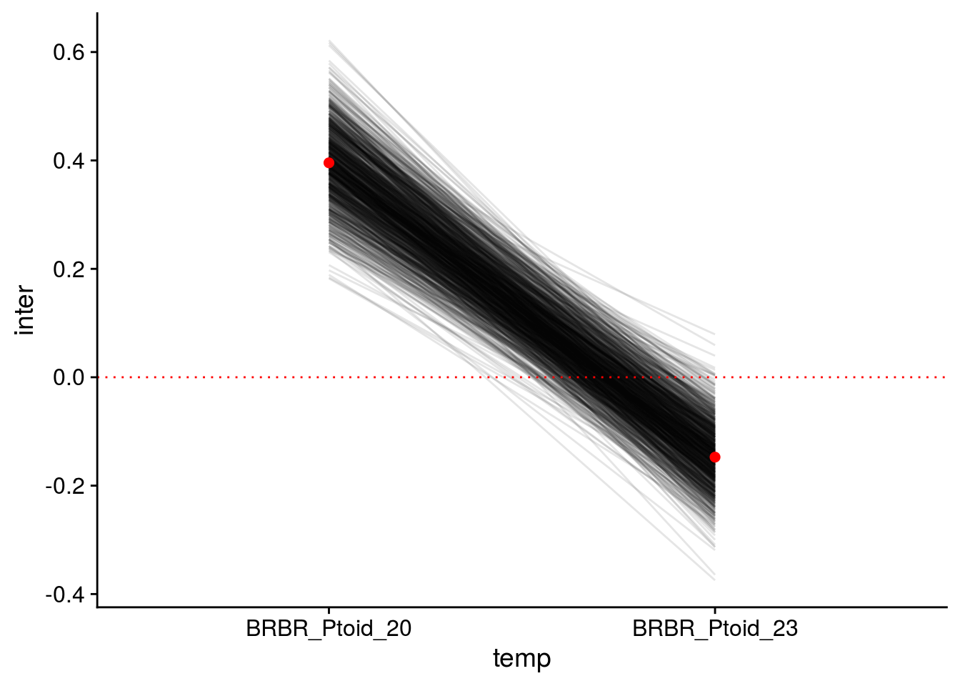

Past versions of unnamed-chunk-12-3.png

Version	Author	Date
86116c8	mabarbour	2020-06-23

# rarely is the parasitoid's intrinsic growth rate estimated as positive, 
# althought it should be negative
pp.temp_model %>%
  mutate(pp_ID = 1:nrow(.),
         r_BRBR_20 = b_log1pPtoidt1_intercept + b_log1pPtoidt1_rich*rich.cond,
         r_BRBR_23 = b_log1pPtoidt1_intercept + b_log1pPtoidt1_rich*rich.cond + b_log1pPtoidt1_temp*3) %>%
  select(pp_ID, r_BRBR_20, r_BRBR_23) %>%
  gather(key = temp, value = r, -pp_ID) %>%
  # use all samples to see occasional unrealistic estimate # filter(pp_ID %in% rsamp) %>% # subsample to avoid crowding plot
  ggplot(., aes(x = temp, y = r)) +
  geom_line(aes(group = pp_ID), alpha = 0.1) +
  stat_summary(fun.y = mean, geom = "point", col = "red", size = 2) +
  geom_hline(yintercept = 0, linetype = "dotted", color = "red")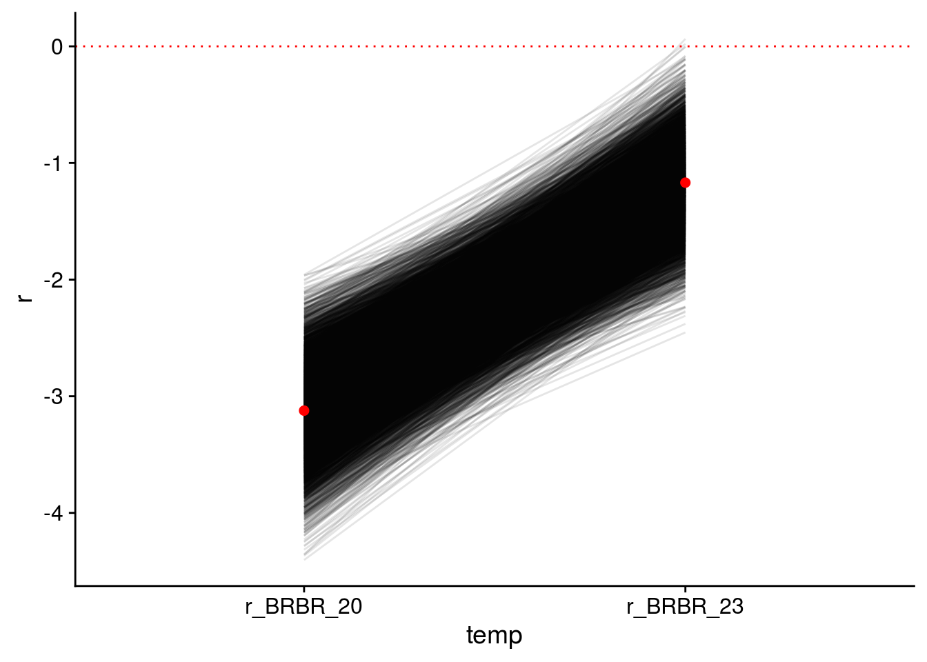 

Past versions of unnamed-chunk-12-4.png

Version	Author	Date
86116c8	mabarbour	2020-06-23

Note that some of the posterior samples can be biologically unfeasible, such as aphids with negative intrinsic growth rates. I restrict our inference to those parameters that are feasible. For example, if an aphid’s intrinsic growth rate was estimated as negative, I manually set it to a small positive value of 0.1. In terms of the interactions, I ensured that any apparent negative effects of aphids on the parasitoids was unrealistic, so I constrained this parameter to be zero or positive.

Note that if I went ahead without this biological restriction, our results remain qualitatively the same.

# get posterior samples of structural stability
temp20C_stability <- apply(
  pp.temp_model, 
  MARGIN = 1, 
  FUN = function(x) { 
    tmp.mat = matrix(c(x["b_log1pBRBRt1_log1pBRBR_t"], 
                       0, 
                       x["b_log1pBRBRt1_log1pPtoid_t"],
                       x["b_log1pLYERt1_log1pBRBR_t"] + x["b_log1pLYERt1_log1pBRBR_t:rich"]*rich.cond, 
                       x["b_log1pLYERt1_log1pLYER_t"], 
                       x["b_log1pLYERt1_log1pPtoid_t"],
                       x["b_log1pPtoidt1_log1pBRBR_t"] + x["b_log1pPtoidt1_log1pBRBR_t:rich"]*rich.cond, 
                       x["b_log1pPtoidt1_log1pLYER_t"], 
                       0),
                     ncol = 3, byrow = TRUE)
    # constrain intraspecific BRBR effect to a max of zero
    if(tmp.mat[1,1] > 0){
       tmp.mat[1,1] <- 0
    }
    # constrain BRBR-Ptoid interaction to a min of zero
    if(tmp.mat[3,1] < 0){
       tmp.mat[3,1] <- 0
    }
    
    tmp.r = matrix(c(x["b_log1pBRBRt1_intercept"],
                     x["b_log1pLYERt1_intercept"] + x["b_log1pLYERt1_rich"]*rich.cond,
                     x["b_log1pPtoidt1_intercept"] + x["b_log1pPtoidt1_rich"]*rich.cond),
                   ncol = 1)
    # constrain BRBR intrinsic growth rate to positive values
    if(tmp.r[1] < 0){
      tmp.r[1] <- 0.1 # small positive value
    }
    # constrain Ptoid intrinsic growth rate to negative values
    if(tmp.r[3] > 0){
      tmp.r[3] <- -0.1 # small negative value
    }
    
    Feasibility = as.numeric(FeasibilityBoundary(tmp.mat, tmp.r)["feasibility"])
    FeasibilityBoundary23 = as.numeric(FeasibilityBoundary(tmp.mat, tmp.r)["alpha.A23"])
    Extinctions = paste0(which(-1*inv(tmp.mat) %*% tmp.r < 0), collapse = ",")
    Resilience = max(Re(eigen((tmp.mat + diag(3)))$values))
    list(tmp.mat = tmp.mat,
         tmp.r = tmp.r,
         Feasibility = Feasibility,
         FeasibilityBoundary23 = FeasibilityBoundary23,
         Extinctions = Extinctions,
         Resilience = Resilience)
  })
temp20C_stability.df <- data.frame(
  temp = "20 C",
  posterior_sample = 1:nrow(pp.temp_model),
  Feasibility = unlist(lapply(temp20C_stability, FUN = function(x) x$Feasibility)),
  FeasibilityBoundary23 = unlist(lapply(temp20C_stability, FUN = function(x) x$FeasibilityBoundary23)),
  Extinctions = unlist(lapply(temp20C_stability, FUN = function(x) x$Extinctions)),
  Resilience = unlist(lapply(temp20C_stability, FUN = function(x) x$Resilience))
)

temp23C_stability <- apply(
  pp.temp_model, 
  MARGIN = 1, 
  FUN = function(x) { 
    tmp.mat = matrix(c(x["b_log1pBRBRt1_log1pBRBR_t"] + x["b_log1pBRBRt1_log1pBRBR_t:temp"]*3, 
                       0, 
                       x["b_log1pBRBRt1_log1pPtoid_t"] + x["b_log1pBRBRt1_log1pPtoid_t:temp"]*3,
                       x["b_log1pLYERt1_log1pBRBR_t"] + x["b_log1pLYERt1_log1pBRBR_t:rich"]*rich.cond, 
                       x["b_log1pLYERt1_log1pLYER_t"], 
                       x["b_log1pLYERt1_log1pPtoid_t"],
                       x["b_log1pPtoidt1_log1pBRBR_t"] + x["b_log1pPtoidt1_log1pBRBR_t:rich"]*rich.cond + x["b_log1pPtoidt1_log1pBRBR_t:temp"]*3, 
                       x["b_log1pPtoidt1_log1pLYER_t"], 
                       0),
                     ncol = 3, byrow = TRUE)
    # constrain intraspecific BRBR effect to a max of zero
    if(tmp.mat[1,1] > 0){
       tmp.mat[1,1] <- 0
    }
    # constrain BRBR-Ptoid interaction to a min of zero
    if(tmp.mat[3,1] < 0){
       tmp.mat[3,1] <- 0
    }
    
    tmp.r = matrix(c(x["b_log1pBRBRt1_intercept"] + x["b_log1pBRBRt1_temp"]*3,
                     x["b_log1pLYERt1_intercept"] + x["b_log1pLYERt1_rich"]*rich.cond,
                     x["b_log1pPtoidt1_intercept"] + x["b_log1pPtoidt1_rich"]*rich.cond + x["b_log1pPtoidt1_temp"]*3),
                   ncol = 1)
    # constrain BRBR intrinsic growth rate to positive values
    if(tmp.r[1] < 0){
      tmp.r[1] <- 0.1 # small positive value
    }
    # constrain Ptoid intrinsic growth rate to negative values
    if(tmp.r[3] > 0){
      tmp.r[3] <- -0.1 # small negative value
    }
    
    Feasibility = as.numeric(FeasibilityBoundary(tmp.mat, tmp.r)["feasibility"])
    FeasibilityBoundary23 = as.numeric(FeasibilityBoundary(tmp.mat, tmp.r)["alpha.A23"])
    Extinctions = paste0(which(-1*inv(tmp.mat) %*% tmp.r < 0), collapse = ",")
    Resilience = max(Re(eigen((tmp.mat + diag(3)))$values))
    list(tmp.mat = tmp.mat,
         tmp.r = tmp.r,
         Feasibility = Feasibility,
         FeasibilityBoundary23 = FeasibilityBoundary23,
         Extinctions = Extinctions,
         Resilience = Resilience)
  })
temp23C_stability.df <- data.frame(
  temp = "23 C",
  posterior_sample = 1:nrow(pp.temp_model),
  Feasibility = unlist(lapply(temp23C_stability, FUN = function(x) x$Feasibility)),
  FeasibilityBoundary23 = unlist(lapply(temp23C_stability, FUN = function(x) x$FeasibilityBoundary23)),
  Extinctions = unlist(lapply(temp23C_stability, FUN = function(x) x$Extinctions)),
  Resilience = unlist(lapply(temp23C_stability, FUN = function(x) x$Resilience))
)


all.temp_stability.df <- bind_rows(temp20C_stability.df, temp23C_stability.df) 

Reproduce Fig. S2

# Boundary determined by LYER-Ptoid (23)
all.temp_stability.df %>%
  filter(posterior_sample %in% rsamp) %>% # plot subset of posterior for easier visualization
  mutate(n.temp = as.numeric(as.factor(temp))) %>% 
  ggplot(., aes(x = n.temp, y = FeasibilityBoundary23)) +
  geom_line(aes(group = posterior_sample), alpha = 0.1) +
  stat_summary(fun.y = mean, geom = "line", color = "red", size = 1) +
  stat_summary(fun.y = mean, geom = "point", color = "red", size = 1.5) +
  theme_minimal_hgrid() +
  scale_x_continuous(name = "Temperature", breaks = c(1,2), labels = c("20 C", "23 C"), expand = c(0.1,0.1)) +
  ylab("Critical boundary (L-P)")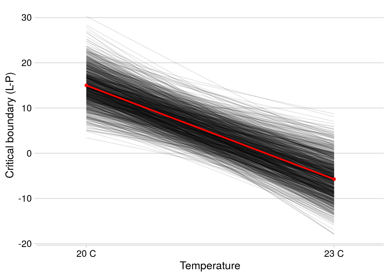

Past versions of unnamed-chunk-14-1.png

Version	Author	Date
86116c8	mabarbour	2020-06-23

## calculate percentage of posterior estimates where temperature decreases structural stability
# organize data
FeasibilityBoundary23_df <- all.temp_stability.df %>%
  select(temp, posterior_sample, FeasibilityBoundary23) %>%
  spread(key = temp, value = FeasibilityBoundary23) %>%
  mutate(Diff = `23 C` - `20 C`)
# calculate percentage
mean(FeasibilityBoundary23_df$Diff < 0)

[1] 1

Non-equilibrium simulation (Fig. S3)

noneq_temp20 <- SimulateCommunityDynamics(IGR.Vector = temp20.IGR, Interaction.Matrix = (temp20.mat + diag(3)), Duration = 9) %>% mutate(temp = "20 C")

noneq_temp23 <- SimulateCommunityDynamics(IGR.Vector = temp23.IGR, Interaction.Matrix = (temp23.mat + diag(3)), Duration = 7) %>% mutate(temp = "23 C")

bind_rows(noneq_temp20, noneq_temp23) %>%
  gather(Species, value = "Abundance", -Week, - temp) %>%
  ggplot(., aes(x = Week, y = Abundance, color = Species)) +
  geom_hline(yintercept = 0, linetype = "dotted") +
  geom_line() +
  geom_point() +
  facet_wrap(~temp, ncol = 1) +
  theme_minimal_hgrid() +
  ylab("Abundance (log scale)") +
  scale_color_viridis_d(labels = c("B. brassicae","L. erysimi","D. rapae"))

Past versions of unnamed-chunk-15-1.png

Version	Author	Date
86116c8	mabarbour	2020-06-23

Save analysis

Write out an .RData file to use for the Supplementary Online Materiak.

save.image(file = "output/structural-stability.RData")

Session information

sessionInfo()

R version 3.6.3 (2020-02-29)
Platform: x86_64-pc-linux-gnu (64-bit)
Running under: Ubuntu 16.04.6 LTS

Matrix products: default
BLAS:   /usr/lib/libblas/libblas.so.3.6.0
LAPACK: /usr/lib/lapack/liblapack.so.3.6.0

locale:
 [1] LC_CTYPE=en_US.UTF-8       LC_NUMERIC=C              
 [3] LC_TIME=en_US.UTF-8        LC_COLLATE=en_US.UTF-8    
 [5] LC_MONETARY=en_US.UTF-8    LC_MESSAGES=en_US.UTF-8   
 [7] LC_PAPER=en_US.UTF-8       LC_NAME=C                 
 [9] LC_ADDRESS=C               LC_TELEPHONE=C            
[11] LC_MEASUREMENT=en_US.UTF-8 LC_IDENTIFICATION=C       

attached base packages:
[1] stats     graphics  grDevices utils     datasets  methods   base     

other attached packages:
 [1] rgl_0.100.54    knitr_1.26      tidybayes_2.0.1 matlib_0.9.2   
 [5] cowplot_1.0.0   forcats_0.4.0   stringr_1.4.0   dplyr_0.8.3    
 [9] purrr_0.3.3     readr_1.3.1     tidyr_1.0.2     tibble_2.1.3   
[13] ggplot2_3.2.1   tidyverse_1.3.0 brms_2.12.7     Rcpp_1.0.2     
[17] RCurl_1.95-4.12 bitops_1.0-6   

loaded via a namespace (and not attached):
  [1] colorspace_1.4-1        ellipsis_0.3.0          rio_0.5.16             
  [4] ggridges_0.5.1          rsconnect_0.8.13        rprojroot_1.3-2        
  [7] markdown_1.1            base64enc_0.1-3         fs_1.3.1               
 [10] rstudioapi_0.10         rstan_2.19.2            svUnit_0.7-12          
 [13] DT_0.6                  mvtnorm_1.0-10          lubridate_1.7.4        
 [16] xml2_1.2.2              bridgesampling_0.6-0    shinythemes_1.1.2      
 [19] bayesplot_1.7.0         jsonlite_1.6            workflowr_1.6.0        
 [22] broom_0.5.2             dbplyr_1.4.2            shiny_1.3.2            
 [25] compiler_3.6.3          httr_1.4.1              backports_1.1.4        
 [28] assertthat_0.2.1        Matrix_1.2-17           lazyeval_0.2.2         
 [31] cli_1.1.0               later_1.0.0             htmltools_0.3.6        
 [34] prettyunits_1.0.2       tools_3.6.3             igraph_1.2.4.1         
 [37] coda_0.19-2             gtable_0.3.0            glue_1.3.1             
 [40] reshape2_1.4.3          carData_3.0-2           cellranger_1.1.0       
 [43] vctrs_0.2.2             nlme_3.1-140            crosstalk_1.0.0        
 [46] xfun_0.9                ps_1.3.0                openxlsx_4.1.0.1       
 [49] rvest_0.3.5             mime_0.7                miniUI_0.1.1.1         
 [52] lifecycle_0.1.0         gtools_3.8.1            MASS_7.3-51.4          
 [55] zoo_1.8-6               scales_1.0.0            colourpicker_1.0       
 [58] hms_0.5.3               promises_1.0.1          Brobdingnag_1.2-6      
 [61] parallel_3.6.3          inline_0.3.15           shinystan_2.5.0        
 [64] curl_4.0                yaml_2.2.0              gridExtra_2.3          
 [67] loo_2.2.0               StanHeaders_2.19.0      stringi_1.4.3          
 [70] dygraphs_1.1.1.6        zip_2.0.3               pkgbuild_1.0.3         
 [73] manipulateWidget_0.10.0 rlang_0.4.4             pkgconfig_2.0.2        
 [76] matrixStats_0.54.0      evaluate_0.14           lattice_0.20-38        
 [79] labeling_0.3            rstantools_2.0.0        htmlwidgets_1.3        
 [82] processx_3.3.1          tidyselect_0.2.5        plyr_1.8.4             
 [85] magrittr_1.5            R6_2.4.0                generics_0.0.2         
 [88] DBI_1.0.0               foreign_0.8-71          pillar_1.4.2           
 [91] haven_2.2.0             whisker_0.3-2           withr_2.1.2            
 [94] xts_0.11-2              abind_1.4-5             car_3.0-3              
 [97] modelr_0.1.5            crayon_1.3.4            arrayhelpers_1.1-0     
[100] rmarkdown_2.0           viridis_0.5.1           grid_3.6.3             
[103] readxl_1.3.1            data.table_1.12.2       callr_3.2.0            
[106] git2r_0.26.1            threejs_0.3.1           reprex_0.3.0           
[109] digest_0.6.20           webshot_0.5.1           xtable_1.8-4           
[112] httpuv_1.5.1            stats4_3.6.3            munsell_0.5.0          
[115] viridisLite_0.3.0       shinyjs_1.0