Bio322.ensembl1
Marie Saitou
8/23/2021
Last updated: 2021-09-10
Checks: 2 0
Knit directory: Bio322/
This reproducible R Markdown analysis was created with workflowr (version 1.6.2). The Checks tab describes the reproducibility checks that were applied when the results were created. The Past versions tab lists the development history.
Great! Since the R Markdown file has been committed to the Git repository, you know the exact version of the code that produced these results.
Great! You are using Git for version control. Tracking code development and connecting the code version to the results is critical for reproducibility.
The results in this page were generated with repository version 899b470. See the Past versions tab to see a history of the changes made to the R Markdown and HTML files.
Note that you need to be careful to ensure that all relevant files for the analysis have been committed to Git prior to generating the results (you can use wflow_publish or wflow_git_commit). workflowr only checks the R Markdown file, but you know if there are other scripts or data files that it depends on. Below is the status of the Git repository when the results were generated:
Ignored files:
    Ignored:    .DS_Store
Note that any generated files, e.g. HTML, png, CSS, etc., are not included in this status report because it is ok for generated content to have uncommitted changes.
These are the previous versions of the repository in which changes were made to the R Markdown (analysis/ensembl1.rmd) and HTML (docs/ensembl1.html) files. If you’ve configured a remote Git repository (see ?wflow_git_remote), click on the hyperlinks in the table below to view the files as they were in that past version.
| File | Version | Author | Date | Message |
|---|---|---|---|---|
| Rmd | 899b470 | mariesaitou | 2021-09-10 | wflow_publish(“analysis/ensembl1.Rmd”) |
| html | f139bdf | mariesaitou | 2021-09-10 | Build site. |
| html | f863fe0 | mariesaitou | 2021-09-10 | Build site. |
| html | c867c58 | mariesaitou | 2021-09-10 | Build site. |
| Rmd | c41e75f | mariesaitou | 2021-09-10 | wflow_publish(“analysis/ensembl1.Rmd”) |
0. Introduction
This is a set of introductory hands-on exercises to get to know more about the genomes of various animals with public databases. These exercises align the learning goals from module 1 and lectures of Bio322. https://www.nmbu.no/course/BIO322
You can submit your answers on Canvas.
Task 1-1 Explore the human genome content
Let’s explore actual genome databases and get to know the genome contents and feature.
Click the following icon. 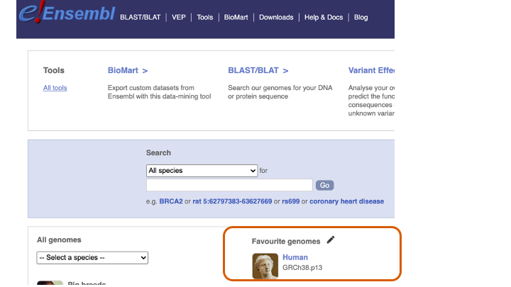
Here, as one example, we are going to look into BRCA2 gene.
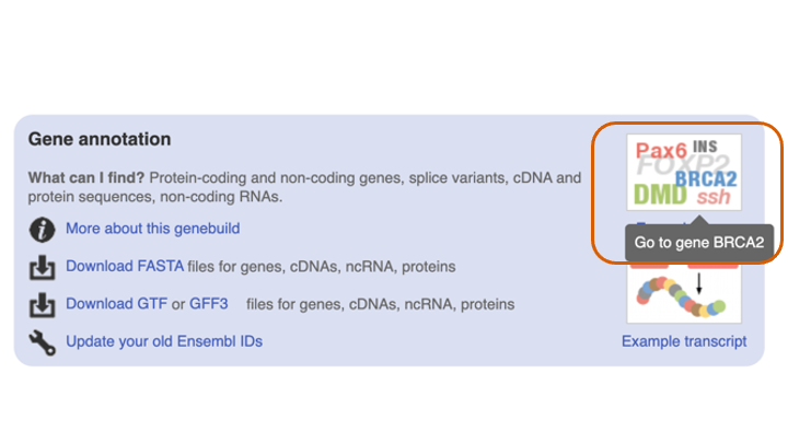
Investigate the BRCA gene as an example
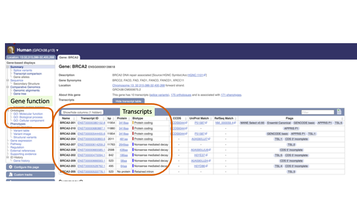
You can see multiple transcripts of the BRCA2 gene
Click “Ontologies” and “Phenotypes” to explore the reported function of this gene.
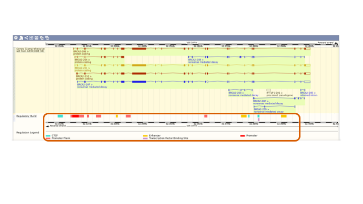
Scroll down to see the transcripts and regulartory regions
Here, there are several questions: ## Question 1 Explore the human genome
- (1-A) What mechanism generates multiple transcripts from one gene?
- (1-B) What is an enhancer, promoter, and transcription factor binding site?
- (1-C) When you want to know function of a gene, what research plan would you make?
Task 1-2 Explore multiple genomes - genome contents
Now, we are going to compare human genome and genomes of other animals.
Go back to the human genome page, and click “(i) More information and statistics”
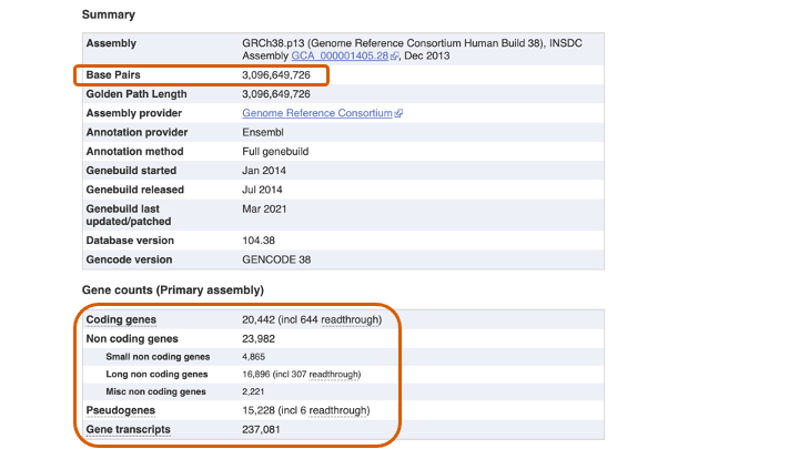
Statistics
Question 2
- (2-A) How much are the Base Pairs, Coding genes, Non-coding genes, Pseudogenes, Gene transcripts in the human genome?
Similarly, let’s explore the genome of
- Chicken
- Common carp
- Saccharomyces cerevisiae (What is its common name??)
and
(2-A, continued) write down: Base Pairs, Coding genes, Non-coding genes, Pseudogenes, Gene transcripts in their genomes. If you are ambitious, make a plot of these.
(2-B) Why is there variation in genome size and gene numbers? How they have been changed in the process of evolution?
(2-C) How do non-coding genes work?
(2-D) What are pseudogenes? How are they generated?
(2-E) Which species has the most genes? What are the advantages of having many genes?
Task 3 Explore multiple genomes - synteny
In this task, we are going to compare the structure of multiple genomes.
SynCircos is a tool to compare the contents of chromosomes from mulciple species. http://bioinfo.konkuk.ac.kr/synteny_portal/
First, compare chromosome 1 of human, gorilla, mouse and cow.

four mammals
We can see that human and gorilla have a quite similar chromosome one content.
However, mouse has only one-third of human chromosome one’s content, and cow’s chromosome one is entirely different from human’s.
So, where in the genome do cow and mouse have human chromosome one’e elements?
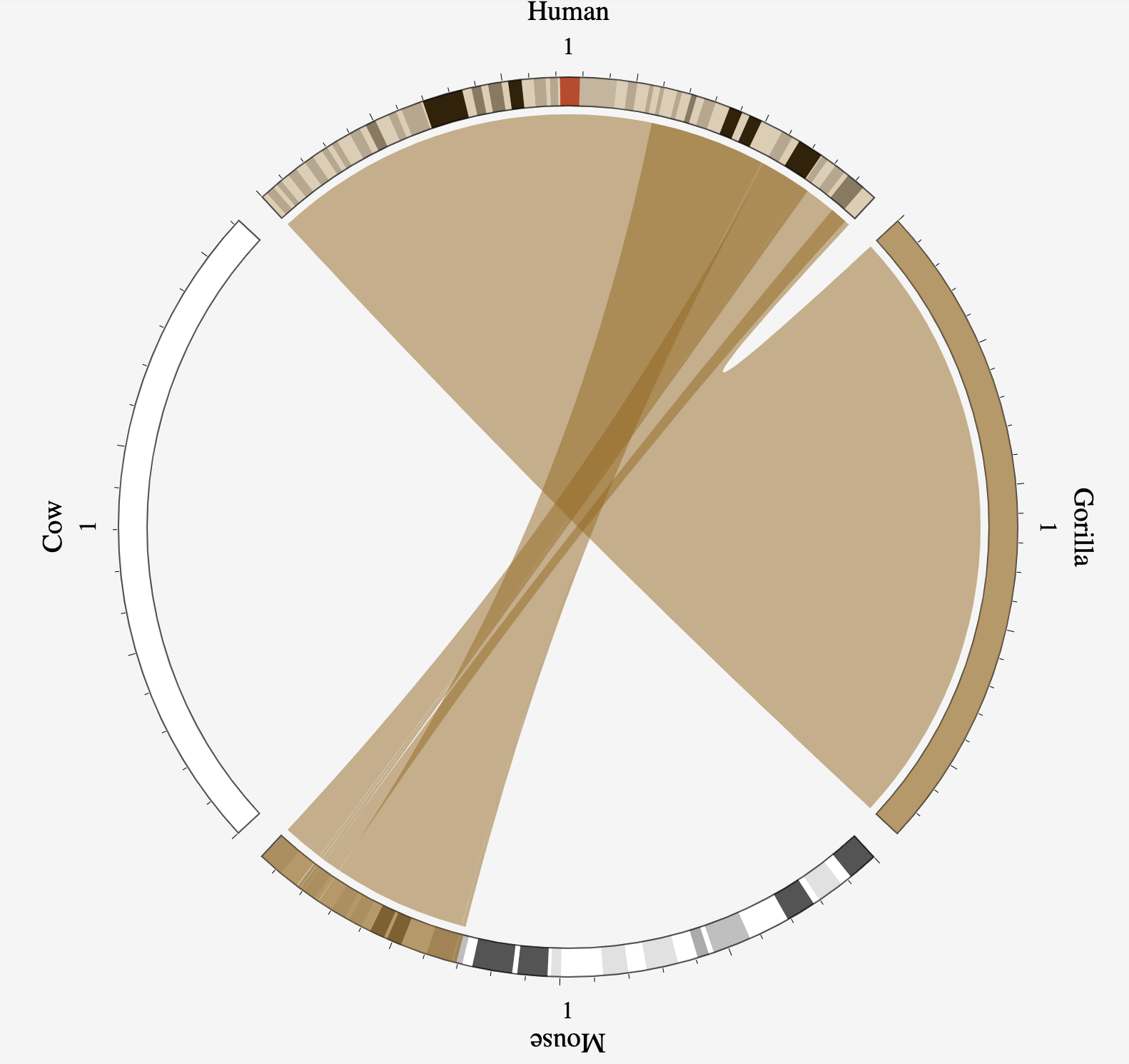
four mammals
Let’s compare human chromosome one and other chromoosmes of mouse and cow.
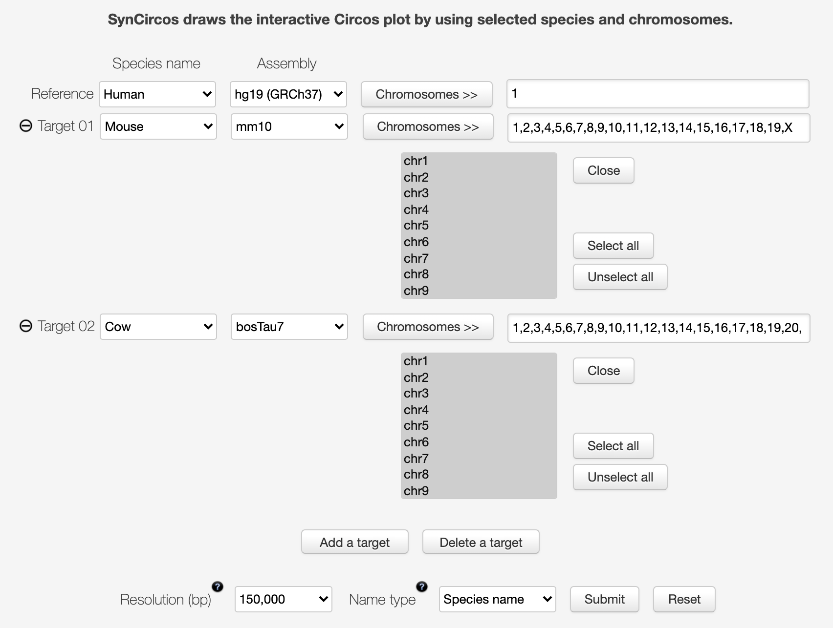
four mammals
And download the result. 
Question 3
- (3-B) Where in the genome do cow and mouse have human chromosome one’s elements?
Task 4 Explore multiple genomes - structure
In this task, we are going to compare the structure of multiple genomes. http://pipmaker.bx.psu.edu/pipmaker/pip-instr.html