The problems up to Problem 3 Part 2 are due Wednesday February 16, 2022 at 11:59pm EST. We'll have the parallel parts (Problem 3, Part 3 and 4) due Tuesday February 22, 2022.

At the time of assignment, we have not covered all the material yet, but I wanted to give you a headstart.

Homework 1 is a chance to get some experience implementing discrete dynamical systems techniques in a way that is parallelized, and a time to understand the fundamental behavior of the bottleneck algorithms in scientific computing.

Please submit the hw to canvas. Canvas will only be used for hw submission. (Original pset authored by Chris Rackauckas.)

Problem 1: A Ton of New Facts on Newton

In this problem we will look into Newton's method. Newton's method is the dynamical system defined by the update process:

\[ x_{n+1} = x_n - \left(\frac{dg}{dx}(x_n)\right)^{-1} g(x_n) \]

For these problems, assume that $\frac{dg}{dx}$ is non-singular.

Part 1

Show that if $x^\ast$ is a steady state of the equation, then $g(x^\ast) = 0$.

Part 2

Take a look at the Quasi-Newton approximation:

\[ x_{n+1} = x_n - \left(\frac{dg}{dx}(x_0)\right)^{-1} g(x_n) \]

for some fixed $x_0$. Derive the stability of the Quasi-Newton approximation in the form of a matrix whose eigenvalues need to be constrained. Use this to argue that if $x_0$ is sufficiently close to $x^\ast$ then the steady state is a stable (attracting) steady state.

Part 3

Relaxed Quasi-Newton is the method:

\[ x_{n+1} = x_n - \alpha \left(\frac{dg}{dx}(x_0)\right)^{-1} g(x_n) \]

Argue that for some sufficiently small $\alpha$ that the Quasi-Newton iterations will be stable if the eigenvalues of $(\left(\frac{dg}{dx}(x_0)\right)^{-1} g(x_n))^\prime$ are all positive for every $x$.

(Technically, these assumptions can be greatly relaxed, but weird cases arise. When $x \in \mathbb{C}$, this holds except on some set of Lebesgue measure zero. Feel free to explore this.)

Part 4

Fixed point iteration is the dynamical system

\[ x_{n+1} = g(x_n) \]

which converges to $g(x)=x$.

1. What is a small change to the dynamical system that could be done such that $g(x)=0$ is the steady state?

2. How can you change the $\left(\frac{dg}{dx}(x_0)\right)^{-1}$ term from the Quasi-Newton iteration to get a method equivalent to fixed point iteration? What does this imply about the difference in stability between Quasi-Newton and fixed point iteration if $\frac{dg}{dx}$ has large eigenvalues?

Problem 2: The Root of all Problems

In this problem we will practice writing fast and type-generic Julia code by producing an algorithm that will compute the quantile of any probability distribution.

Part 1

Many problems can be interpreted as a rootfinding problem. For example, let's take a look at a problem in statistics. Let $X$ be a random variable with a cumulative distribution function (CDF) of $cdf(x)$. Recall that the CDF is a monotonically increasing function in $[0,1]$ which is the total probability of $X < x$. The $y$th quantile of $X$ is the value $x$ at with $X$ has a y% chance of being less than $x$. Interpret the problem of computing an arbitrary quantile $y$ as a rootfinding problem, and use Newton's method to write an algorithm for computing $x$.

(Hint: Recall that $cdf^{\prime}(x) = pdf(x)$, the probability distribution function.)

Part 2

Use the types from Distributions.jl to write a function my_quantile(y,d) which uses multiple dispatch to compute the $y$th quantile for any UnivariateDistribution d from Distributions.jl. Test your function on Gamma(5, 1), Normal(0, 1), and Beta(2, 4) against the Distributions.quantile function built into the library.

(Hint: Have a keyword argument for $x_0$, and let its default be the mean or median of the distribution.)

Problem 3: Bifurcating Data for Parallelism

In this problem we will write code for efficient generation of the bifurcation diagram of the logistic equation.

Part 1

The logistic equation is the dynamical system given by the update relation:

\[ x_{n+1} = rx_n (1-x_n) \]

where $r$ is some parameter. Write a function which iterates the equation from $x_0 = 0.25$ enough times to be sufficiently close to its long-term behavior (400 iterations) and samples 150 points from the steady state attractor (i.e. output iterations 401:550) as a function of $r$, and mutates some vector as a solution, i.e. calc_attractor!(out,f,p,num_attract=150;warmup=400).

Test your function with $r = 2.9$. Double check that your function computes the correct result by calculating the analytical steady state value.

Part 2

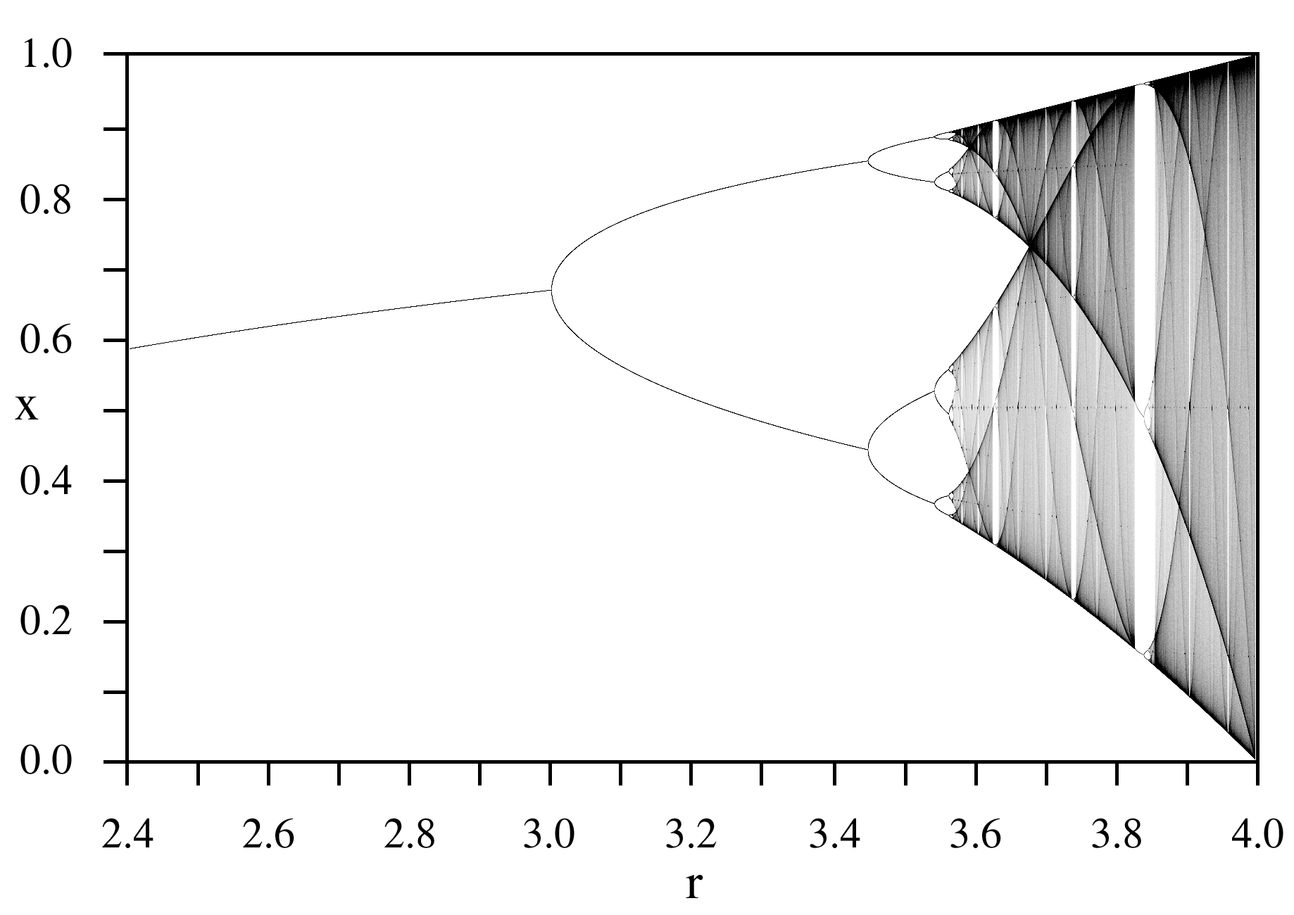
The bifurcation plot shows how a steady state changes as a parameter changes. Compute the long-term result of the logistic equation at the values of r = 2.9:0.001:4, and plot the steady state values for each $r$ as an r x steady_attractor scatter plot. You should get a very bizarrely awesome picture, the bifurcation graph of the logistic equation.

(Hint: Generate a single matrix for the attractor values, and use calc_attractor! on views of columns for calculating the output, or inline the calc_attractor! computation directly onto the matrix, or even give calc_attractor! an input for what column to modify.)

Part 3

Multithread your bifurcation graph generator by performing different steady state calcuations on different threads. Does your timing improve? Why? Be careful and check to make sure you have more than 1 thread!

Part 4

Multiprocess your bifurcation graph generator first by using pmap, and then by using @distributed. Does your timing improve? Why? Be careful to add processes before doing the distributed call.

(Note: You may need to change your implementation around to be allocating differently in order for it to be compatible with multiprocessing!)

Part 5

Which method is the fastest? Why?

---