Forward and Reverse Automatic Differentiation In A Nutshell
Chris Rackauckas
January 21st, 2022
Machine Epsilon and Roundoff Error
Floating point arithmetic is relatively scaled, which means that the precision that you get from calculations is relative to the size of the floating point numbers. Generally, you have 16 digits of accuracy in (64-bit) floating point operations. To measure this, we define machine epsilon as the value by which 1 + E = 1. For floating point numbers, this is:
eps(Float64)
2.220446049250313e-16
However, since it's relative, this value changes as we change our reference value:
@show eps(1.0)
@show eps(0.1)
@show eps(0.01)
eps(1.0) = 2.220446049250313e-16
eps(0.1) = 1.3877787807814457e-17
eps(0.01) = 1.734723475976807e-18
1.734723475976807e-18
Thus issues with roundoff error come when one subtracts out the higher digits. For example, $(x + \epsilon) - x$ should just be $\epsilon$ if there was no roundoff error, but if $\epsilon$ is small then this kicks in. If $x = 1$ and $\epsilon$ is of size around $10^{-10}$, then $x+ \epsilon$ is correct for 10 digits, dropping off the smallest 6 due to error in the addition to $1$. But when you subtract off $x$, you don't get those digits back, and thus you only have 6 digits of $\epsilon$ correct.
Let's see this in action:
ϵ = 1e-10rand()
@show ϵ
@show (1+ϵ)
ϵ2 = (1+ϵ) - 1
(ϵ - ϵ2)
ϵ = 9.236209819962081e-11
1 + ϵ = 1.0000000000923621
-1.975420506320867e-17
See how $\epsilon$ is only rebuilt at accuracy around $10^{-16}$ and thus we only keep around 6 digits of accuracy when it's generated at the size of around $10^{-10}$!
Finite Differencing and Numerical Stability
To start understanding how to compute derivatives on a computer, we start with finite differencing. For finite differencing, recall that the definition of the derivative is:
\[ f'(x) = \lim_{\epsilon \rightarrow 0} \frac{f(x+\epsilon)-f(x)}{\epsilon} \]
Finite differencing directly follows from this definition by choosing a small $\epsilon$. However, choosing a good $\epsilon$ is very difficult. If $\epsilon$ is too large than there is error since this definition is asymtopic. However, if $\epsilon$ is too small, you receive roundoff error. To understand why you would get roundoff error, recall that floating point error is relative, and can essentially store 16 digits of accuracy. So let's say we choose $\epsilon = 10^{-6}$. Then $f(x+\epsilon) - f(x)$ is roughly the same in the first 6 digits, meaning that after the subtraction there is only 10 digits of accuracy, and then dividing by $10^{-6}$ simply brings those 10 digits back up to the correct relative size.

This means that we want to choose $\epsilon$ small enough that the $\mathcal{O}(\epsilon^2)$ error of the truncation is balanced by the $O(1/\epsilon)$ roundoff error. Under some minor assumptions, one can argue that the average best point is $\sqrt(E)$, where E is machine epsilon
@show eps(Float64)
@show sqrt(eps(Float64))
eps(Float64) = 2.220446049250313e-16
sqrt(eps(Float64)) = 1.4901161193847656e-8
1.4901161193847656e-8
This means we should not expect better than 8 digits of accuracy, even when things are good with finite differencing.

The centered difference formula is a little bit better, but this picture suggests something much better...
Differencing in a Different Dimension: Complex Step Differentiation
The problem with finite differencing is that we are mixing our really small number with the really large number, and so when we do the subtract we lose accuracy. Instead, we want to keep the small perturbation completely separate.
To see how to do this, assume that $x \in \mathbb{R}$ and assume that $f$ is complex analytic. You want to calculate a real derivative, but your function just happens to also be complex analytic when extended to the complex plane. Thus it has a Taylor series, and let's see what happens when we expand out this Taylor series purely in the complex direction:
\[ f(x+ih) = f(x) + f'(x)ih + \mathcal{O}(h^2) \]
which we can re-arrange as:
\[ if'(x) = \frac{f(x+ih) - f(x)}{h} + \mathcal{O}(h) \]
Since $x$ is real and $f$ is real-valued on the reals, $if'$ is purely imaginary. So let's take the imaginary parts of both sides:
\[ f'(x) = \frac{Im(f(x+ih))}{h} + \mathcal{O}(h) \]
since $Im(f(x)) = 0$ (since it's real valued!). Thus with a sufficiently small choice of $h$, this is the complex step differentiation formula for calculating the derivative.
But to understand the computational advantage, recal that $x$ is pure real, and thus $x+ih$ is an imaginary number where the $h$ never directly interacts with $x$ since a complex number is a two dimensional number where you keep the two pieces separate. Thus there is no numerical cancellation by using a small value of $h$, and thus, due to the relative precision of floating point numbers, both the real and imaginary parts will be computed to (approximately) 16 digits of accuracy for any choice of $h$.
Derivatives as nilpotent sensitivities
The derivative measures the sensitivity of a function, i.e. how much the function output changes when the input changes by a small amount $\epsilon$:
\[ f(a + \epsilon) = f(a) + f'(a) \epsilon + o(\epsilon). \]
In the following we will ignore higher-order terms; formally we set $\epsilon^2 = 0$. This form of analysis can be made rigorous through a form of non-standard analysis called Smooth Infinitesimal Analysis [1], though note that nilpotent infinitesimal requires constructive logic, and thus proof by contradiction is not allowed in this logic due to a lack of the law of the excluded middle.
A function $f$ will be represented by its value $f(a)$ and derivative $f'(a)$, encoded as the coefficients of a degree-1 (Taylor) polynomial in $\epsilon$:
\[ f \rightsquigarrow f(a) + \epsilon f'(a) \]
Conversely, if we have such an expansion in $\epsilon$ for a given function $f$, then we can identify the coefficient of $\epsilon$ as the derivative of $f$.
Dual numbers
Thus, to extend the idea of complex step differentiation beyond complex analytic functions, we define a new number type, the dual number. A dual number is a multidimensional number where the sensitivity of the function is propagated along the dual portion.
Here we will now start to use $\epsilon$ as a dimensional signifier, like $i$, $j$, or $k$ for quaternion numbers. In order for this to work out, we need to derive an appropriate algebra for our numbers. To do this, we will look at Taylor series to make our algebra reconstruct differentiation.
Note that the chain rule has been explicitly encoded in the derivative part.
\[ f(a + \epsilon) = f(a) + \epsilon f'(a) \]
to first order. If we have two functions
\[ f \rightsquigarrow f(a) + \epsilon f'(a) \]
\[ g \rightsquigarrow g(a) + \epsilon g'(a) \]
then we can manipulate these Taylor expansions to calculate combinations of these functions as follows. Using the nilpotent algebra, we have that:
\[ (f + g) = [f(a) + g(a)] + \epsilon[f'(a) + g'(a)] \]
\[ (f \cdot g) = [f(a) \cdot g(a)] + \epsilon[f(a) \cdot g'(a) + g(a) \cdot f'(a) ] \]
From these we can infer the derivatives by taking the component of $\epsilon$. These also tell us the way to implement these in the computer.
Computer representation
Setup (not necessary from the REPL):
using InteractiveUtils # only needed when using Weave
Each function requires two pieces of information and some particular "behavior", so we store these in a struct. It's common to call this a "dual number":
struct Dual{T}
    val::T   # value
    der::T  # derivative
end
Each Dual object represents a function. We define arithmetic operations to mirror performing those operations on the corresponding functions.
We must first import the operations from Base:
Base.:+(f::Dual, g::Dual) = Dual(f.val + g.val, f.der + g.der)
Base.:+(f::Dual, α::Number) = Dual(f.val + α, f.der)
Base.:+(α::Number, f::Dual) = f + α

#=
You can also write:
import Base: +
f::Dual + g::Dual = Dual(f.val + g.val, f.der + g.der)
=#

Base.:-(f::Dual, g::Dual) = Dual(f.val - g.val, f.der - g.der)

# Product Rule
Base.:*(f::Dual, g::Dual) = Dual(f.val*g.val, f.der*g.val + f.val*g.der)
Base.:*(α::Number, f::Dual) = Dual(f.val * α, f.der * α)
Base.:*(f::Dual, α::Number) = α * f

# Quotient Rule
Base.:/(f::Dual, g::Dual) = Dual(f.val/g.val, (f.der*g.val - f.val*g.der)/(g.val^2))
Base.:/(α::Number, f::Dual) = Dual(α/f.val, -α*f.der/f.val^2)
Base.:/(f::Dual, α::Number) = f * inv(α) # Dual(f.val/α, f.der * (1/α))

Base.:^(f::Dual, n::Integer) = Base.power_by_squaring(f, n)  # use repeated squaring for integer powers
We can now define Duals and manipulate them:
f = Dual(3, 4)
g = Dual(5, 6)

f + g
Main.##WeaveSandBox#1023.Dual{Int64}(8, 10)
f * g
Main.##WeaveSandBox#1023.Dual{Int64}(15, 38)
f * (g + g)
Main.##WeaveSandBox#1023.Dual{Int64}(30, 76)
Defining Higher Order Primitives
We can also define functions of Dual objects, using the chain rule. To speed up our derivative function, we can directly hardcode the derivative of known functions which we call primitives. If f is a Dual representing the function $f$, then exp(f) should be a Dual representing the function $\exp \circ f$, i.e. with value $\exp(f(a))$ and derivative $(\exp \circ f)'(a) = \exp(f(a)) \, f'(a)$:
import Base: exp
exp(f::Dual) = Dual(exp(f.val), exp(f.val) * f.der)
exp (generic function with 36 methods)
f
Main.##WeaveSandBox#1023.Dual{Int64}(3, 4)
exp(f)
Main.##WeaveSandBox#1023.Dual{Float64}(20.085536923187668, 80.3421476927506
7)
Differentiating arbitrary functions
For functions where we don't have a rule, we can recursively do dual number arithmetic within the function until we hit primitives where we know the derivative, and then use the chain rule to propagate the information back up. Under this algebra, we can represent $a + \epsilon$ as Dual(a, 1). Thus, applying f to Dual(a, 1) should give Dual(f(a), f'(a)). This is thus a 2-dimensional number for calculating the derivative without floating point error, using the compiler to transform our equations into dual number arithmetic. To to differentiate an arbitrary function, we define a generic function and then change the algebra.
h(x) = x^2 + 2
a = 3
xx = Dual(a, 1)
Main.##WeaveSandBox#1023.Dual{Int64}(3, 1)
Now we simply evaluate the function h at the Dual number xx:
h(xx)
Main.##WeaveSandBox#1023.Dual{Int64}(11, 6)
The first component of the resulting Dual is the value $h(a)$, and the second component is the derivative, $h'(a)$!
We can codify this into a function as follows:
derivative(f, x) = f(Dual(x, one(x))).der
derivative (generic function with 1 method)
Here, one is the function that gives the value $1$ with the same type as that of x.
Finally we can now calculate derivatives such as
derivative(x -> 3x^5 + 2, 2)
240
As a bigger example, we can take a pure Julia sqrt function and differentiate it by changing the internal algebra:
function newtons(x)
   a = x
   for i in 1:300
       a = 0.5 * (a + x/a)
   end
   a
end
@show newtons(2.0)
@show (newtons(2.0+sqrt(eps())) - newtons(2.0))/ sqrt(eps())
newtons(Dual(2.0,1.0))
newtons(2.0) = 1.414213562373095
(newtons(2.0 + sqrt(eps())) - newtons(2.0)) / sqrt(eps()) = 0.3535533994436
264
Main.##WeaveSandBox#1023.Dual{Float64}(1.414213562373095, 0.353553390593273
73)
Higher dimensions
How can we extend this to higher dimensional functions? For example, we wish to differentiate the following function $f: \mathbb{R}^2 \to \mathbb{R}$:
ff(x, y) = x^2 + x*y
ff (generic function with 1 method)
Recall that the partial derivative $\partial f/\partial x$ is defined by fixing $y$ and differentiating the resulting function of $x$:
a, b = 3.0, 4.0

ff_1(x) = ff(x, b)  # single-variable function
ff_1 (generic function with 1 method)
Since we now have a single-variable function, we can differentiate it:
derivative(ff_1, a)
10.0
Under the hood this is doing
ff(Dual(a, one(a)), b)
Main.##WeaveSandBox#1023.Dual{Float64}(21.0, 10.0)
Similarly, we can differentiate with respect to $y$ by doing
ff_2(y) = ff(a, y)  # single-variable function

derivative(ff_2, b)
3.0
Note that we must do two separate calculations to get the two partial derivatives; in general, calculating the gradient $\nabla$ of a function $f:\mathbb{R}^n \to \mathbb{R}$ requires $n$ separate calculations.
Implementation of higher-dimensional forward-mode AD
We can implement derivatives of functions $f: \mathbb{R}^n \to \mathbb{R}$ by adding several independent partial derivative components to our dual numbers.
We can think of these as $\epsilon$ perturbations in different directions, which satisfy $\epsilon_i^2 = \epsilon_i \epsilon_j = 0$, and we will call $\epsilon$ the vector of all perturbations. Then we have
\[ f(a + \epsilon) = f(a) + \nabla f(a) \cdot \epsilon + \mathcal{O}(\epsilon^2), \]
where $a \in \mathbb{R}^n$ and $\nabla f(a)$ is the gradient of $f$ at $a$, i.e. the vector of partial derivatives in each direction. $\nabla f(a) \cdot \epsilon$ is the directional derivative of $f$ in the direction $\epsilon$.
We now proceed similarly to the univariate case:
\[ (f + g)(a + \epsilon) = [f(a) + g(a)] + [\nabla f(a) + \nabla g(a)] \cdot \epsilon \]
\[ \begin{align} (f \cdot g)(a + \epsilon) &= [f(a) + \nabla f(a) \cdot \epsilon ] \, [g(a) + \nabla g(a) \cdot \epsilon ] \\ &= f(a) g(a) + [f(a) \nabla g(a) + g(a) \nabla f(a)] \cdot \epsilon. \end{align} \]
We will use the StaticArrays.jl package for efficient small vectors:
using StaticArrays

struct MultiDual{N,T}
    val::T
    derivs::SVector{N,T}
end

import Base: +, *

function +(f::MultiDual{N,T}, g::MultiDual{N,T}) where {N,T}
    return MultiDual{N,T}(f.val + g.val, f.derivs + g.derivs)
end

function *(f::MultiDual{N,T}, g::MultiDual{N,T}) where {N,T}
    return MultiDual{N,T}(f.val * g.val, f.val .* g.derivs + g.val .* f.derivs)
end
* (generic function with 694 methods)
gg(x, y) = x*x*y + x + y

(a, b) = (1.0, 2.0)

xx = MultiDual(a, SVector(1.0, 0.0))
yy = MultiDual(b, SVector(0.0, 1.0))

gg(xx, yy)
Main.##WeaveSandBox#1023.MultiDual{2, Float64}(5.0, [5.0, 2.0])
We can calculate the Jacobian of a function $\mathbb{R}^n \to \mathbb{R}^m$ by applying this to each component function:
ff(x, y) = SVector(x*x + y*y , x + y)

ff(xx, yy)
2-element SVector{2, Main.##WeaveSandBox#1023.MultiDual{2, Float64}} with i
ndices SOneTo(2):
 Main.##WeaveSandBox#1023.MultiDual{2, Float64}(5.0, [2.0, 4.0])
 Main.##WeaveSandBox#1023.MultiDual{2, Float64}(3.0, [1.0, 1.0])
It would be possible (and better for performance in many cases) to store all of the partials in a matrix instead.
Forward-mode AD is implemented in a clean and efficient way in the ForwardDiff.jl package:
using ForwardDiff, StaticArrays

ForwardDiff.gradient( xx -> ( (x, y) = xx; x^2 * y + x*y ), [1, 2])
2-element Vector{Int64}:
 6
 2
Directional derivative and gradient of functions $f: \mathbb{R}^n \to \mathbb{R}$
For a function $f: \mathbb{R}^n \to \mathbb{R}$ the basic operation is the directional derivative:
\[ \lim_{\epsilon \to 0} \frac{f(\mathbf{x} + \epsilon \mathbf{v}) - f(\mathbf{x})}{\epsilon} = [\nabla f(\mathbf{x})] \cdot \mathbf{v}, \]
where $\epsilon$ is still a single dimension and $\nabla f(\mathbf{x})$ is the direction in which we calculate.
We can directly do this using the same simple Dual numbers as above, using the same $\epsilon$, e.g.
\[ f(x, y) = x^2 \sin(y) \]
\[ \begin{align} f(x_0 + a\epsilon, y_0 + b\epsilon) &= (x_0 + a\epsilon)^2 \sin(y_0 + b\epsilon) \\ &= x_0^2 \sin(y_0) + \epsilon[2ax_0 \sin(y_0) + x_0^2 b \cos(y_0)] + o(\epsilon) \end{align} \]
so we have indeed calculated $\nabla f(x_0, y_0) \cdot \mathbf{v},$ where $\mathbf{v} = (a, b)$ are the components that we put into the derivative component of the Dual numbers.
If we wish to calculate the directional derivative in another direction, we could repeat the calculation with a different $\mathbf{v}$. A better solution is to use another independent epsilon $\epsilon$, expanding $x = x_0 + a_1 \epsilon_1 + a_2 \epsilon_2$ and putting $\epsilon_1 \epsilon_2 = 0$.
In particular, if we wish to calculate the gradient itself, $\nabla f(x_0, y_0)$, we need to calculate both partial derivatives, which corresponds to two directional derivatives, in the directions $(1, 0)$ and $(0, 1)$, respectively.
Forward-Mode AD as jvp
Note that another representation of the directional derivative is $f'(x)v$, where $f'(x)$ is the Jacobian or total derivative of $f$ at $x$. To see the equivalence of this to a directional derivative, first let's see an example:
\[ \left[\begin{array}{ccc} \frac{\partial f_{1}}{\partial x_{1}} & \frac{\partial f_{1}}{\partial x_{2}} & \frac{\partial f_{1}}{\partial x_{3}}\\ \frac{\partial f_{2}}{\partial x_{1}} & \frac{\partial f_{2}}{\partial x_{2}} & \frac{\partial f_{2}}{\partial x_{3}}\\ \frac{\partial f_{3}}{\partial x_{1}} & \frac{\partial f_{3}}{\partial x_{2}} & \frac{\partial f_{3}}{\partial x_{3}}\\ \frac{\partial f_{4}}{\partial x_{1}} & \frac{\partial f_{4}}{\partial x_{2}} & \frac{\partial f_{4}}{\partial x_{3}}\\ \frac{\partial f_{5}}{\partial x_{1}} & \frac{\partial f_{5}}{\partial x_{2}} & \frac{\partial f_{5}}{\partial x_{3}} \end{array}\right]\left[\begin{array}{c} v_{1}\\ v_{2}\\ v_{3} \end{array}\right]=\left[\begin{array}{c} \frac{\partial f_{1}}{\partial x_{1}}v_{1}+\frac{\partial f_{1}}{\partial x_{2}}v_{2}+\frac{\partial f_{1}}{\partial x_{3}}v_{3}\\ \frac{\partial f_{2}}{\partial x_{1}}v_{1}+\frac{\partial f_{2}}{\partial x_{2}}v_{2}+\frac{\partial f_{2}}{\partial x_{3}}v_{3}\\ \frac{\partial f_{3}}{\partial x_{1}}v_{1}+\frac{\partial f_{3}}{\partial x_{2}}v_{2}+\frac{\partial f_{3}}{\partial x_{3}}v_{3}\\ \frac{\partial f_{4}}{\partial x_{1}}v_{1}+\frac{\partial f_{4}}{\partial x_{2}}v_{2}+\frac{\partial f_{4}}{\partial x_{3}}v_{3}\\ \frac{\partial f_{5}}{\partial x_{1}}v_{1}+\frac{\partial f_{5}}{\partial x_{2}}v_{2}+\frac{\partial f_{5}}{\partial x_{3}}v_{3} \end{array}\right]=\left[\begin{array}{c} \nabla f_{1}(x)\cdot v\\ \nabla f_{2}(x)\cdot v\\ \nabla f_{3}(x)\cdot v\\ \nabla f_{4}(x)\cdot v\\ \nabla f_{5}(x)\cdot v \end{array}\right] \]
Or more formally, let's write it out in the standard basis:
\[ w_i = \sum_{j}^{m} J_{ij} v_{j} \]
Now write out what $J$ means and we see that:
\[ w_i = \sum_j^{m} \frac{df_i}{dx_j} v_j = \nabla f_i(x) \cdot v \]
The primitive action of forward-mode AD is f'(x)v!
This is also known as a Jacobian-vector product, or jvp for short.
We can thus represent vector calculus with multidimensional dual numbers as follows. Let $d =[x,y]$, the vector of dual numbers. We can instead represent this as:
\[ d = d_0 + v_1 \epsilon_1 + v_2 \epsilon_2 \]
where $d_0$ is the primal vector $[x_0,y_0]$ and the $v_i$ are the vectors for the dual directions. If you work out this algebra, then note that a single application of $f$ to a multidimensional dual number calculates:
\[ f(d) = f(d_0) + f'(d_0)v_1 \epsilon_1 + f'(d_0)v_2 \epsilon_2 \]
i.e. it calculates the result of $f(x,y)$ and two separate directional derivatives. Note that because the information about $f(d_0)$ is shared between the calculations, this is more efficient than doing multiple applications of $f$. And of course, this is then generalized to $m$ many directional derivatives at once by:
\[ d = d_0 + v_1 \epsilon_1 + v_2 \epsilon_2 + \ldots + v_m \epsilon_m \]
Jacobian
For a function $f: \mathbb{R}^n \to \mathbb{R}^m$, we reduce (conceptually, although not necessarily in code) to its component functions $f_i: \mathbb{R}^n \to \mathbb{R}$, where $f(x) = (f_1(x), f_2(x), \ldots, f_m(x))$.
Then
\[ \begin{align} f(x + \epsilon v) &= (f_1(x + \epsilon v), \ldots, f_m(x + \epsilon v)) \\ &= (f_1(x) + \epsilon[\nabla f_1(x) \cdot v], \dots, f_m(x) + \epsilon[\nabla f_m(x) \cdot v] \\ &= f(x) + [f'(x) \cdot v] \epsilon, \end{align} \]
To calculate the complete Jacobian, we calculate these directional derivatives in the $n$ different directions of the basis vectors, i.e. if
\[ d = d_0 + e_1 \epsilon_1 + \ldots + e_n \epsilon_n \]
for $e_i$ the $i$th basis vector, then
\[ f(d) = f(d_0) + Je_1 \epsilon_1 + \ldots + Je_n \epsilon_n \]
computes all columns of the Jacobian simultaniously.
Forward-Mode Automatic Differentiation for Gradients
Let's recall the forward-mode method for computing gradients. For an arbitrary nonlinear function $f$ with scalar output, we can compute derivatives by putting a dual number in. For example, with
\[ d = d_0 + v_1 \epsilon_1 + \ldots + v_m \epsilon_m \]
we have that
\[ f(d) = f(d_0) + f'(d_0)v_1 \epsilon_1 + \ldots + f'(d_0)v_m \epsilon_m \]
where $f'(d_0)v_i$ is the direction derivative in the direction of $v_i$. To compute the gradient with respond to the input, we thus need to make $v_i = e_i$.
However, in this case we now do not want to compute the derivative with respect to the input! Instead, now we have $f(x;p)$ and want to compute the derivatives with respect to $p$. This simply means that we want to take derivatives in the directions of the parameters. To do this, let:
\[ x = x_0 + 0 \epsilon_1 + \ldots + 0 \epsilon_k \]
\[ P = p + e_1 \epsilon_1 + \ldots + e_k \epsilon_k \]
where there are $k$ parameters. We then have that
\[ f(x;P) = f(x;p) + \frac{df}{dp_1} \epsilon_1 + \ldots + \frac{df}{dp_k} \epsilon_k \]
as the output, and thus a $k+1$-dimensional number computes the gradient of the function with respect to $k$ parameters.
Can we do better?
Reverse-Mode Automatic Differentiation
The fast method for computing gradients goes under many times. The adjoint technique, backpropogation, and reverse-mode automatic differentiation are in some sense all equivalent phrases given to this method from different disciplines. To understand this technique, first let's understand programs $f$ as a composition of $L$ functions:
\[ f = f^L \circ f^{L-1} \circ \ldots \circ f^1 \]
This should be intuitive because a program is just breaking down the steps of a calculation, like:
x = 5 + 2
y = x * 3
z = x ^ y
558545864083284007
could have simply been written as:
(5+2) ^ ((5+2)*3)
558545864083284007
Composing the assignment statements together gives the mathematical form of the function as a composition of the intermediate calculations. Now if $f$ is
\[ f = f^L \circ f^{L-1} \circ \ldots \circ f^1 \]
then the Jacobian matrix satisfies:
\[ J = J_L J_{L-1} \ldots J_1 \]
This fact is just another way of writing the chain rule:
\[ (g(f(x)))' = g'(f(x))*f'(x) = J_2 * J_1 \]
Forward-mode automatic differentiation worked by propogating forward the actions of the Jacobians at every step of the program:
\[ Jv = J_L (J_{L-1} (\ldots (J_1 v) \ldots )) \]
effectively calculating the Jacobian of the program by multiplying by the Jacobians from left to right at each step of the way. This means doing primitive $Jv$ calculations on each underlying problem, and pushing that calculation through. When the primitive of a function was unknown, one would dig into how that function was defined, recursively, until primitive derivative definitions were known and used to define the dual part. Thus primitives defined how deep into a calculation one would look for an analytical solution to $J_i v$, and then the automatic differentiation engine would simply chain together these Jacobian-vector products.
Forward-mode accumulation was good because $Jv$ directly calculated the directional derivative, which is also seen as the columns of the Jacobian (in a chosen basis). However, the key to understanding reverse-mode automatic differentiation is to see that gradients are the rows of the Jacobian. Let's see this in an example:
\[ \left[\begin{array}{ccccc} 0 & 1 & 0 & 0 & 0\end{array}\right]\left[\begin{array}{ccc} \frac{\partial f_{1}}{\partial x_{1}} & \frac{\partial f_{1}}{\partial x_{2}} & \frac{\partial f_{1}}{\partial x_{3}}\\ \frac{\partial f_{2}}{\partial x_{1}} & \frac{\partial f_{2}}{\partial x_{2}} & \frac{\partial f_{2}}{\partial x_{3}}\\ \frac{\partial f_{3}}{\partial x_{1}} & \frac{\partial f_{3}}{\partial x_{2}} & \frac{\partial f_{3}}{\partial x_{3}}\\ \frac{\partial f_{4}}{\partial x_{1}} & \frac{\partial f_{4}}{\partial x_{2}} & \frac{\partial f_{4}}{\partial x_{3}}\\ \frac{\partial f_{5}}{\partial x_{1}} & \frac{\partial f_{5}}{\partial x_{2}} & \frac{\partial f_{5}}{\partial x_{3}} \end{array}\right]=\left[\begin{array}{ccc} \frac{\partial f_{2}}{\partial x_{1}} & \frac{\partial f_{2}}{\partial x_{2}} & \frac{\partial f_{2}}{\partial x_{3}}\end{array}\right]=\nabla f_{2}(x) \]
Notice that multiplying by a row vector [0 1 0 0 0] pulls out the second row of the Jacobian, which pulls out the gradient of the second component of the multi-output function. If f(x) is a function that returned a scalar, [1] * J would give $\nabla f(x)$. Thus if we want to calculate gradients fast, we need to do automatic differentiation in a way that computes one row at a time, not one column at a time, and for scalar outputs then the gradient can be calculated in O(1) time instead of O(n)!
However, this matrix calculus understanding of reverse-mode automatic differentiation directly describes how it gets its name. We can thus think of this as a different direction for the Jacobian accumulation. Let's see what happens when we left apply a row vector to the Jacobian, but recurse down to the component $J_i$ pieces of a composed function:
\[ v^T J = (\ldots ((v^T J_L) J_{L-1}) \ldots ) J_1 \]
Multiplying on the right does $J_1 v$ first, while multiplying on the left requires doing $v^T J_L$ first. This means in order to do this calcaultion, the derivative must be computed in reverse starting from the end, giving rise to the name reverse-mode AD. We must chain together vector-Jacobian product, or vjp calculations from the last step of the calculation to the previous all the way back to the start.
Quick note on notation
Some people write reverse-mode AD as the $J^T v$ action, but you can also see this implies reverse accumulation by the properties of the transpose since
\[ J^T v = (J_L J_{L-1} \ldots J_1)^T v = (J_1^T J_{2}^T \ldots J_L^T )v \]
the transpose reverses the order of multiplication.
Okay, now let's figure out how to do the calculation in this style.
Reverse-Mode of a Neural Network
Let's do reverse-mode automatic differentiation fo the following function:
\[ \begin{align} z &= W_1 x + b_1\\ h &= \sigma(z)\\ y &= W_2 h + b_2\\ \mathcal{L} &= \frac{1}{2} \Vert y-t \Vert^2 \end{align} \]
where we call $f(x) = L$. To simplify our notation, let's write for $y = f(x)$ the simplification:
\[ \overline{x} = [\frac{\partial f}{\partial x}]^T v \]
The reason is because we want to encode the successive "$J'v$ of last time" expressions. To calculate $f'(x)^T v$ we decompose it into steps $(J_1^T J_{2}^T \ldots J_L^T )v$, or:
\[ \begin{align} \overline{L} &= v\\ \overline{y} &= [\frac{\partial (\frac{1}{2} \Vert y-t \Vert^2)}{\partial y}]^T \overline{L} = (y-t)^T v\\ \overline{h} &= [\frac{\partial (W_2 h + b_2)}{\partial h}]^T \overline{y} = W_2^T \overline{y}\\ \overline{z} &= [\frac{\partial \sigma(z)}{\partial z}]^T \overline{h} = \sigma^\prime(z)^T \overline{h}\\ \overline{x} &= [\frac{\partial W_1 x + b_1}{\partial x}]^T \overline{z} = W_1^T \overline{z}\\ \end{align} \]
(note that since $L$ is a scalar, $v$ is a scalar here so we don't really need to transpose, that's more to show form). Or, in order to calculate $f'(x)^T v$, we do this by calculating:
\[ J^T v = (W_1^T \sigma^\prime(z)^T W_2^T (y-t)^T) v \]
and if $v=1$ then we receive the gradient of the neural network with respect to $x$.
Primitives of Reverse Mode
For forward-mode AD, we saw that we could define primitives in order to accelerate the calculation. For example, knowing that
\[ exp(x+\epsilon) = exp(x) + exp(x)\epsilon \]
allows the program to skip autodifferentiating through the code for exp. This was simple with forward-mode since we could represent the operation on a Dual number. What's the equivalent for reverse-mode AD? The answer is the pullback function. If $y = [y_1,y_2,\ldots] = f(x_1,x_2, \ldots)$, then $[\overline{x_1},\overline{x_2},\ldots]=\mathcal{B}_f^x(\overline{y})$ is the pullback of $f$ at the point $x$, defined for a scalar loss function $L(y)$ as:
\[ \overline{x_i} = \frac{\partial L}{\partial x} = \sum_i \frac{\partial L}{\partial y_i} \frac{\partial y_i}{\partial x_i} \]
Using the notation from earlier, $\overline{y} = \frac{\partial L}{\partial y}$ is the derivative of the some intermediate w.r.t. the cost function, and thus
\[ \overline{x_i} = \sum_i \overline{y_i} \frac{\partial y_i}{\partial x_i} = \mathcal{B}_f^x(\overline{y}) \]
Note that $\mathcal{B}_f^x(\overline{y})$ is a function of $x$ because the reverse pass that is use embeds values from the forward pass, and the values from the forward pass to use are those calculated during the evaluation of $f(x)$.
By the chain rule, if we don't have a primitive defined for $y_i(x)$, we can compute that by $\mathcal{B}_{y_i}(\overline{y})$, and recursively apply this process until we hit rules that we know. The rules to start with are the scalar derivative rules with follow quite simply, and the multivariate rules which we derived above. For example, if $y=f(x)=Ax$, then
\[ \mathcal{B}_{f}^x(\overline{y}) = \overline{y}^T A \]
which is simply saying that the Jacobian of $f$ at $x$ is $A$, and so the vjp is to multiply the vector transpose by $A$.
Likewise, for element-wise operations, the Jacobian is diagonal, and thus the vjp is multiplying once again by a diagonal matrix against the derivative, deriving the same pullback as we had for backpropogation in a neural network. This then is a quicker encoding and derivation of backpropogation.
Example of a Reverse-Mode AD Primitive
Let's write down the reverse-mode primitive for $y = \sigma(Wx + b)$. Doing as we showed before, we break down the steps of the computation and write the $J'v$ one step at a time until we get back to the start:
using ChainRules
nndense(W,x,b) = σ.(W*x + b)
function ChainRules.rrule(::typeof(nndense), W,x,b)
  r = W*x .+ b
  y = σ.(r)

  function adjoint(v)
    zbar = ForwardDiff.derivative.(f.σ,r) .* v
    xbar = W' * zbar
    NoTangent(),NotImplemented(),xbar,NotImplemented()
  end
  y,adjoint
end
The homework will be to figure out how to calculate Wbar and bbar!
Forward Mode vs Reverse Mode Efficiency
Notice that a pullback of a single scalar gives the gradient of a function, while the pushforward using forward-mode of a dual gives a directional derivative. Forward mode computes columns of a Jacobian, while reverse mode computes gradients (rows of a Jacobian). Therefore, the relative efficiency of the two approaches is based on the size of the Jacobian. If $f:\mathbb{R}^n \rightarrow \mathbb{R}^m$, then the Jacobian is of size $m \times n$. If $m$ is much smaller than $n$, then computing by each row will be faster, and thus use reverse mode. In the case of a gradient, $m=1$ while $n$ can be large, leading to this phonomena. Likewise, if $n$ is much smaller than $m$, then computing by each column will be faster. We will see shortly the reverse mode AD has a high overhead with respect to forward mode, and thus if the values are relatively equal (or $n$ and $m$ are small), forward mode is more efficient.
However, since optimization needs gradients, reverse-mode definitely has a place in the standard toolchain which is why backpropagation is so central to machine learning. But this does not mean that reverse-mode AD is "faster", in fact for square matrices it's usually slower!.
Extra: Reverse-Mode Automatic Differentiation on Computation Graphs
Most lecture notes will show reverse-mode automatic differentiation on computation graphs as the core way to do the calculation because they want to avoid matrix calculus. The following walks through that approach to show how it's a very tedious way to derive the same results.
Adjoints and Reverse-Mode AD through Computation Graphs
Let's look at the multivariate chain rule on a computation graph. Recall that for $f(x(t),y(t))$ that we have:
\[ \frac{df}{dt} = \frac{df}{dx}\frac{dx}{dt} + \frac{df}{dy}\frac{dy}{dt} \]
We can visualize our direct dependences as the computation graph:
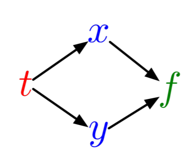
i.e. $t$ directly determines $x$ and $y$ which then determines $f$. To calculate Assume you've already evaluated $f(t)$. If this has been done, then you've already had to calculate $x$ and $y$. Thus given the function $f$, we can now calculate $\frac{df}{dx}$ and $\frac{df}{dy}$, and then calculate $\frac{dx}{dt}$ and $\frac{dy}{dt}$.
Now let's put another layer in the computation. Let's make $f(x(v(t),w(t)),y(v(t),w(t))$. We can write out the full expression for the derivative. Notice that even with this additional layer, the statement we wrote above still holds:
\[ \frac{df}{dt} = \frac{df}{dx}\frac{dx}{dt} + \frac{df}{dy}\frac{dy}{dt} \]
So given an evaluation of $f$, we can (still) directly calculate $\frac{df}{dx}$ and $\frac{df}{dy}$. But now, to calculate $\frac{dx}{dt}$ and $\frac{dy}{dt}$, we do the next step of the chain rule:
\[ \frac{dx}{dt} = \frac{dx}{dv}\frac{dv}{dt} + \frac{dx}{dw}\frac{dw}{dt} \]
and similar for $y$. So plug it all in, and you see that our equations will grow wild if we actually try to plug it in! But it's clear that, to calculate $\frac{df}{dt}$, we can first calculate $\frac{df}{dx}$, and then multiply that to $\frac{dx}{dt}$. If we had more layers, we could calculate the sensitivity (the derivative) of the output to the last layer, then and then the sensitivity to the second layer back is the sensitivity of the last layer multiplied to that, and the third layer back has the sensitivity of the second layer multiplied to it!
Logistic Regression Example
To better see this structure, let's write out a simple example. Let our forward pass through our function be:
\[ \begin{align} z &= wx + b\\ y &= \sigma(z)\\ \mathcal{L} &= \frac{1}{2}(y-t)^2\\ \mathcal{R} &= \frac{1}{2}w^2\\ \mathcal{L}_{reg} &= \mathcal{L} + \lambda \mathcal{R}\end{align} \]
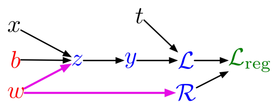
The formulation of the program here is called a Wengert list, tape, or graph. In this, $x$ and $t$ are inputs, $b$ and $W$ are parameters, $z$, $y$, $\mathcal{L}$, and $\mathcal{R}$ are intermediates, and $\mathcal{L}_{reg}$ is our output.
This is a simple univariate logistic regression model. To do logistic regression, we wish to find the parameters $w$ and $b$ which minimize the distance of $\mathcal{L}_{reg}$ from a desired output, which is done by computing derivatives.
Let's calculate the derivatives with respect to each quantity in reverse order. If our program is $f(x) = \mathcal{L}_{reg}$, then we have that
\[ \frac{df}{\mathcal{L}_{reg}} = 1 \]
as the derivatives of the last layer. To computerize our notation, let's write
\[ \overline{\mathcal{L}_{reg}} = \frac{df}{\mathcal{L}_{reg}} \]
for our computed values. For the derivatives of the second to last layer, we have that:
\[ \begin{align} \overline{\mathcal{R}} &= \frac{df}{\mathcal{L}_{reg}} \frac{d\mathcal{L}_{reg}}{\mathcal{R}}\\ &= \overline{\mathcal{L}_{reg}} \lambda \end{align} \]
\[ \begin{align} \overline{\mathcal{L}} &= \frac{df}{\mathcal{L}_{reg}} \frac{d\mathcal{L}_{reg}}{\mathcal{L}}\\ &= \overline{\mathcal{L}_{reg}} \end{align} \]
This was our observation from before that the derivative of the second layer is the partial derivative of the current values times the sensitivity of the final layer. And then we keep multiplying, so now for our next layer we have that:
\[ \begin{align} \overline{y} &= \overline{\mathcal{L}} \frac{d\mathcal{L}}{dy}\\ &= \overline{\mathcal{L}} (y-t) \end{align} \]
And notice that the chain rule holds since $\overline{\mathcal{L}}$ implicitly already has the multiplication by $\overline{\mathcal{L}_{reg}}$ inside of it. Then the next layer is:
\[ \begin{align} \frac{df}{z} &= \overline{y} \frac{dy}{dz}\\ &= \overline{y} \sigma^\prime(z) \end{align} \]
Then the next layer. Notice that here, by the chain rule on $w$ we have that:
\[ \begin{align} \overline{w} &= \overline{z} \frac{\partial z}{\partial w} + \overline{\mathcal{R}} \frac{d \mathcal{R}}{dw}\\ &= \overline{z} x + \overline{\mathcal{R}} w\end{align} \]
\[ \begin{align} \overline{b} &= \overline{z} \frac{\partial z}{\partial b}\\ &= \overline{z} \end{align} \]
This completely calculates all derivatives. In conclusion, the rule is:
You sum terms from each outward arrow
Each arrow has the derivative term of the end times the partial of the current term.
Recurse backwards to build simple linear combination expressions.
Quick note
We started this derivation with
\[ \frac{df}{\mathcal{L}_{reg}} = 1 \]
and we then get out $\nabla f(x)$, but from our discussion before this is simply [1]' J. Thus while we have a (flaky) justification for making this value 1, it's really just the choice of $v$! Thus doing
\[ \frac{df}{\mathcal{L}_{reg}} = v \]
will make this process compute $v^T J$ for this $f$.
Backpropogation of a Neural Network
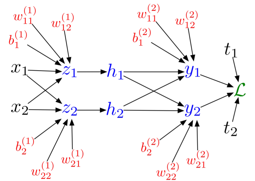
Now let's look at backpropgation of a deep neural network. Before getting to it in the linear algebraic sense, let's write everything in terms of scalars. This means we can write a simple neural network as:
\[ \begin{align} z_i &= \sum_j W_{ij}^1 x_j + b_i^1\\ h_i &= \sigma(z_i)\\ y_i &= \sum_j W_{ij}^2 h_j + b_i^2\\ \mathcal{L} &= \frac{1}{2} \sum_k \left(y_k - t_k \right)^2 \end{align} \]
where I have chosen the L2 loss function. This is visualized by the computational graph:
Then we can do the same process as before to get:
\[ \begin{align} \overline{\mathcal{L}} &= 1\\ \overline{y_i} &= \overline{\mathcal{L}} (y_i - t_i)\\ \overline{w_{ij}^2} &= \overline{y_i} h_j\\ \overline{b_i^2} &= \overline{y_i}\\ \overline{h_i} &= \sum_k (\overline{y_k}w_{ki}^2)\\ \overline{z_i} &= \overline{h_i}\sigma^\prime(z_i)\\ \overline{w_{ij}^1} &= \overline{z_i} x_j\\ \overline{b_i^1} &= \overline{z_i}\end{align} \]
just by examining the computation graph. Now let's write this in linear algebraic form.
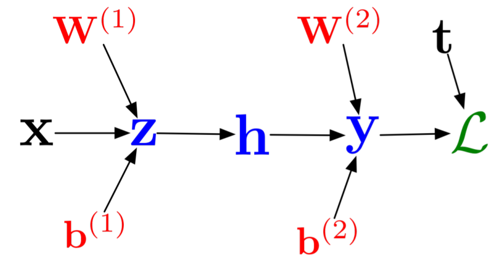
The forward pass for this simple neural network was:
\[ \begin{align} z &= W_1 x + b_1\\ h &= \sigma(z)\\ y &= W_2 h + b_2\\ \mathcal{L} = \frac{1}{2} \Vert y-t \Vert^2 \end{align} \]
If we carefully decode our scalar expression, we see that we get the following:
\[ \begin{align} \overline{\mathcal{L}} &= 1\\ \overline{y} &= \overline{\mathcal{L}}(y-t)\\ \overline{W_2} &= \overline{y}h^{T}\\ \overline{b_2} &= \overline{y}\\ \overline{h} &= W_2^T \overline{y}\\ \overline{z} &= \overline{h} .* \sigma^\prime(z)\\ \overline{W_1} &= \overline{z} x^T\\ \overline{b_1} &= \overline{z} \end{align} \]
We can thus decode the rules as:
Multiplying by the matrix going forwards means multiplying by the transpose going backwards. A term on the left stays on the left, and a term on the right stays on the right.
Element-wise operations give element-wise multiplication
Notice that the summation is then easily encoded into this rule by the transpose operation.
We can write it in the general DNN form of:
\[ r_i = W_i v_{i} + b_i \]
\[ v_{i+1} = \sigma_i.(r_i) \]
\[ v_1 = x \]
\[ \mathcal{L} = \frac{1}{2} \Vert v_{n} - t \Vert \]
\[ \begin{align} \overline{\mathcal{L}} &= 1\\ \overline{v_n} &= \overline{\mathcal{L}}(y-t)\\ \overline{r_i} &= \overline{v_i} .* \sigma_i^\prime (r_i)\\ \overline{W_i} &= \overline{v_i}r_{i-1}^{T}\\ \overline{b_i} &= \overline{v_i}\\ \overline{v_{i-1}} &= W_{i}^{T} \overline{v_i} \end{align} \]
References
John L. Bell, An Invitation to Smooth Infinitesimal Analysis, http://publish.uwo.ca/~jbell/invitation%20to%20SIA.pdf
Bell, John L. A Primer of Infinitesimal Analysis
Nocedal & Wright, Numerical Optimization, Chapter 8
Griewank & Walther, Evaluating Derivatives