Knowles 2019 data
ERM
2023-06-21
Last updated: 2023-06-21
Checks: 7 0
Knit directory: Cardiotoxicity/
This reproducible R Markdown analysis was created with workflowr (version 1.7.0). The Checks tab describes the reproducibility checks that were applied when the results were created. The Past versions tab lists the development history.
Great! Since the R Markdown file has been committed to the Git repository, you know the exact version of the code that produced these results.
Great job! The global environment was empty. Objects defined in the global environment can affect the analysis in your R Markdown file in unknown ways. For reproduciblity it’s best to always run the code in an empty environment.
The command set.seed(20230109) was run prior to running
the code in the R Markdown file. Setting a seed ensures that any results
that rely on randomness, e.g. subsampling or permutations, are
reproducible.
Great job! Recording the operating system, R version, and package versions is critical for reproducibility.
Nice! There were no cached chunks for this analysis, so you can be confident that you successfully produced the results during this run.
Great job! Using relative paths to the files within your workflowr project makes it easier to run your code on other machines.
Great! You are using Git for version control. Tracking code development and connecting the code version to the results is critical for reproducibility.
The results in this page were generated with repository version 347bf4c. See the Past versions tab to see a history of the changes made to the R Markdown and HTML files.
Note that you need to be careful to ensure that all relevant files for
the analysis have been committed to Git prior to generating the results
(you can use wflow_publish or
wflow_git_commit). workflowr only checks the R Markdown
file, but you know if there are other scripts or data files that it
depends on. Below is the status of the Git repository when the results
were generated:
Ignored files:
    Ignored:    .RData
    Ignored:    .Rhistory
    Ignored:    .Rproj.user/
    Ignored:    data/41588_2018_171_MOESM3_ESMeQTL_ST2_for paper.csv
    Ignored:    data/Arr_GWAS.txt
    Ignored:    data/Arr_geneset.RDS
    Ignored:    data/BC_cell_lines.csv
    Ignored:    data/CADGWASgene_table.csv
    Ignored:    data/CAD_geneset.RDS
    Ignored:    data/Clamp_Summary.csv
    Ignored:    data/Cormotif_24_k1-5_raw.RDS
    Ignored:    data/DAgostres24.RDS
    Ignored:    data/DAtable1.csv
    Ignored:    data/DDEMresp_list.csv
    Ignored:    data/DDE_reQTL.txt
    Ignored:    data/DDEresp_list.csv
    Ignored:    data/DEG-GO/
    Ignored:    data/DEG_cormotif.RDS
    Ignored:    data/DF_Plate_Peak.csv
    Ignored:    data/DRC48hoursdata.csv
    Ignored:    data/Da24counts.txt
    Ignored:    data/Dx24counts.txt
    Ignored:    data/Dx_reQTL_specific.txt
    Ignored:    data/Ep24counts.txt
    Ignored:    data/GOIsig.csv
    Ignored:    data/GOplots.R
    Ignored:    data/GTEX_setsimple.csv
    Ignored:    data/GTEx_gene_list.csv
    Ignored:    data/HFGWASgene_table.csv
    Ignored:    data/HF_geneset.RDS
    Ignored:    data/Heart_Left_Ventricle.v8.egenes.txt
    Ignored:    data/Hf_GWAS.txt
    Ignored:    data/K_cluster
    Ignored:    data/K_cluster_kisthree.csv
    Ignored:    data/K_cluster_kistwo.csv
    Ignored:    data/LDH48hoursdata.csv
    Ignored:    data/Mt24counts.txt
    Ignored:    data/RINsamplelist.txt
    Ignored:    data/Seonane2019supp1.txt
    Ignored:    data/TOP2Bi-24hoursGO_analysis.csv
    Ignored:    data/TR24counts.txt
    Ignored:    data/Top2biresp_cluster24h.csv
    Ignored:    data/Viabilitylistfull.csv
    Ignored:    data/allexpressedgenes.txt
    Ignored:    data/allgenes.txt
    Ignored:    data/allmatrix.RDS
    Ignored:    data/avgLD50.RDS
    Ignored:    data/backGL.txt
    Ignored:    data/cormotif_3hk1-8.RDS
    Ignored:    data/cormotif_initalK5.RDS
    Ignored:    data/cormotif_initialK5.RDS
    Ignored:    data/cormotif_initialall.RDS
    Ignored:    data/counts24hours.RDS
    Ignored:    data/cpmcount.RDS
    Ignored:    data/cpmnorm_counts.csv
    Ignored:    data/crispr_genes.csv
    Ignored:    data/cvd_GWAS.txt
    Ignored:    data/dat_cpm.RDS
    Ignored:    data/data_outline.txt
    Ignored:    data/efit2.RDS
    Ignored:    data/efit2results.RDS
    Ignored:    data/ensembl_backup.RDS
    Ignored:    data/ensgtotal.txt
    Ignored:    data/filenameonly.txt
    Ignored:    data/filtered_cpm_counts.csv
    Ignored:    data/filtered_raw_counts.csv
    Ignored:    data/filtermatrix_x.RDS
    Ignored:    data/folder_05top/
    Ignored:    data/geneDoxonlyQTL.csv
    Ignored:    data/gene_corr_frame.RDS
    Ignored:    data/gene_prob_tran3h.RDS
    Ignored:    data/gene_probabilityk5.RDS
    Ignored:    data/gostresTop2bi_ER.RDS
    Ignored:    data/gostresTop2bi_LR
    Ignored:    data/gostresTop2bi_LR.RDS
    Ignored:    data/gostresTop2bi_TI.RDS
    Ignored:    data/gostrescoNR
    Ignored:    data/gtex/
    Ignored:    data/heartgenes.csv
    Ignored:    data/individualDRCfile.RDS
    Ignored:    data/individual_DRC48.RDS
    Ignored:    data/individual_LDH48.RDS
    Ignored:    data/knowfig4.csv
    Ignored:    data/knowfig5.csv
    Ignored:    data/mymatrix.RDS
    Ignored:    data/nonresponse_cluster24h.csv
    Ignored:    data/norm_LDH.csv
    Ignored:    data/norm_counts.csv
    Ignored:    data/old_sets/
    Ignored:    data/plan2plot.png
    Ignored:    data/raw_counts.csv
    Ignored:    data/response_cluster24h.csv
    Ignored:    data/sigVDA24.txt
    Ignored:    data/sigVDA3.txt
    Ignored:    data/sigVDX24.txt
    Ignored:    data/sigVDX3.txt
    Ignored:    data/sigVEP24.txt
    Ignored:    data/sigVEP3.txt
    Ignored:    data/sigVMT24.txt
    Ignored:    data/sigVMT3.txt
    Ignored:    data/sigVTR24.txt
    Ignored:    data/sigVTR3.txt
    Ignored:    data/siglist.RDS
    Ignored:    data/slope_table.csv
    Ignored:    data/table3a.omar
    Ignored:    data/toplistall.RDS
    Ignored:    data/tvl24hour.txt
    Ignored:    data/tvl24hourw.txt
    Ignored:    data/venn_code.R

Untracked files:
    Untracked:  .RDataTmp
    Untracked:  .RDataTmp1
    Untracked:  .RDataTmp2
    Untracked:  OmicNavigator_learn.R
    Untracked:  code/DRC_plotfigure1.png
    Untracked:  code/cpm_boxplot.R
    Untracked:  code/fig1plot.png
    Untracked:  code/figurelegeddrc.png
    Untracked:  cormotif_probability_genelist.csv
    Untracked:  individual-legenddark2.png
    Untracked:  installed_old.rda
    Untracked:  motif_ER.txt
    Untracked:  motif_LR.txt
    Untracked:  motif_NR.txt
    Untracked:  motif_TI.txt
    Untracked:  output/Doxonly_deg.csv
    Untracked:  output/daplot.RDS
    Untracked:  output/dxplot.RDS
    Untracked:  output/epplot.RDS
    Untracked:  output/mtplot.RDS
    Untracked:  output/output-old/
    Untracked:  output/trplot.RDS
    Untracked:  output/veplot.RDS
    Untracked:  reneebasecode.R

Unstaged changes:
    Modified:   analysis/GTEx_genes.Rmd
    Modified:   analysis/LDH_analysis.Rmd
    Modified:   analysis/other_analysis.Rmd
Note that any generated files, e.g. HTML, png, CSS, etc., are not included in this status report because it is ok for generated content to have uncommitted changes.
These are the previous versions of the repository in which changes were
made to the R Markdown (analysis/Knowles2019.Rmd) and HTML
(docs/Knowles2019.html) files. If you’ve configured a
remote Git repository (see ?wflow_git_remote), click on the
hyperlinks in the table below to view the files as they were in that
past version.
| File | Version | Author | Date | Message |
|---|---|---|---|---|
| Rmd | 347bf4c | reneeisnowhere | 2023-06-21 | adding in Doxspecific to graph |
| html | 7749676 | reneeisnowhere | 2023-06-20 | Build site. |
| Rmd | c26c27b | reneeisnowhere | 2023-06-20 | updating titles on graphs |
| html | a77fd98 | reneeisnowhere | 2023-06-20 | Build site. |
| Rmd | 4c762a8 | reneeisnowhere | 2023-06-20 | adding Dox specific investigation |
| Rmd | e94e8f2 | reneeisnowhere | 2023-06-19 | new code from Monday |
| html | 124e036 | reneeisnowhere | 2023-06-16 | Build site. |
| Rmd | fd4fe27 | reneeisnowhere | 2023-06-16 | fix spelling |
| html | d6ad3fe | reneeisnowhere | 2023-06-16 | Build site. |
| Rmd | 4191e24 | reneeisnowhere | 2023-06-16 | adding lcpm plots for dox spec |
| html | bd0e45f | reneeisnowhere | 2023-06-15 | Build site. |
| Rmd | af93421 | reneeisnowhere | 2023-06-15 | adding in seperate files |
| Rmd | 1a1a034 | reneeisnowhere | 2023-06-15 | updates galore |
| Rmd | f8f511a | reneeisnowhere | 2023-06-15 | updates and simplifications of code |
| Rmd | 7fc7ec7 | reneeisnowhere | 2023-06-14 | updating code |
package loading
function load
Knowles data
The code below is how I wrangled the knowles supplemental lists into entrezgene_ids to overlap with my expressed gene lists
Enrichment of Pairwise
backGL <- read.csv("data/backGL.txt",     row.names =1)
drug_palNoVeh <- c("#8B006D","#DF707E","#F1B72B", "#3386DD","#707031")
drug_palc <- c("#8B006D","#DF707E","#F1B72B", "#3386DD","#707031","#41B333")
time <- rep((rep(c("3h", "24h"), c(6,6))), 6)
time <- ordered(time, levels =c("3h", "24h"))
drug <- rep(c("Daunorubicin","Doxorubicin","Epirubicin","Mitoxantrone","Trastuzumab", "Vehicle"),12)
mat_drug <- c("Daunorubicin","Doxorubicin","Epirubicin","Mitoxantrone")
indv <- as.factor(rep(c(1,2,3,4,5,6), c(12,12,12,12,12,12)))
labeltop <- (interaction(substring(drug, 0, 2), indv, time))
level_order2 <- c('75','87','77','79','78','71')


toplistall <- readRDS("data/toplistall.RDS")
knowles4 <-readRDS("output/knowles4.RDS")
knowles5 <-readRDS("output/knowles5.RDS")
DOXmeSNPs <- readRDS("output/DOXmeSNPs.RDS")
DOXreQTLs <- readRDS("output/DOXreQTLs.RDS")
DNRmeSNPs <- readRDS("output/DNRmeSNPs.RDS")
DNRreQTLs <- readRDS("output/DNRreQTLs.RDS")
EPImeSNPs <- readRDS("output/EPImeSNPs.RDS")
EPIreQTLs <- readRDS("output/EPIreQTLs.RDS")
MTXmeSNPs <- readRDS("output/MTXmeSNPs.RDS")
MTXreQTLs <- readRDS("output/MTXreQTLs.RDS")

toplist24hr <-   toplistall %>%
  mutate(id = as.factor(id)) %>%
  mutate(time=factor(time, levels=c("3_hours","24_hours"))) %>%
  filter(time=="24_hours")

toplist3hr <-   toplistall %>%
  mutate(id = as.factor(id)) %>%
  mutate(time=factor(time, levels=c("3_hours","24_hours"))) %>%
  filter(time=="3_hours")
Determining the genetic basis of anthracycline-cardiotoxicity by
molecular response QTL mapping in induced cardiomyocytes
David A Knowles, Courtney K Burrows†, John D Blischak, Kristen M
Patterson, Daniel J Serie, Nadine Norton, Carole Ober, Jonathan K
Pritchard, Yoav Gilad
Knowles \(~~et~ al.~\) eLife 2018;7:e33480. DOI: https://doi.org/10.7554/eLife.33480
My first question was about transcriptional response at the 24 hour mark with my treatments. 3 hour RNA-seq had low numbers of DEGs,so my initial focus is at 24 hours. This time also happens to be when the Knowles paper collected their RNA-seq data.
Supplementary 4 contains a list of 518 SNPs within 1 Mb of TSS, which had a detectable marginal effect on expression (5% FDR). When converted from ensembl gene id to entrez gene id, my list of genes for this supplement = 521. I will call these meSNPS for marginal effect QTLs.
Supplementary 5 contains a list of 376 response eQTLs (reQTLs). These are variants that were associated with modulation of transcriptomic response to doxorubicin treatment. After database name conversion, I have 377 genes.
meSNPdf <- toplistall %>%
  mutate(id = as.factor(id)) %>%
  mutate(time=factor(time, levels=c("3_hours","24_hours"))) %>%
  mutate(sigcount = if_else(adj.P.Val < 0.05,'sig','notsig'))%>%
  mutate(meSNP = if_else( ENTREZID %in% knowles4$entrezgene_id, "y" , "no")) %>%
  dplyr::select(ENTREZID,id,time,meSNP,sigcount) %>%
  group_by(id,time,meSNP,sigcount) %>%
  tally() %>%
  pivot_wider(id_cols = c(id,time,sigcount), names_from = meSNP,names_glue = "meSNP_{meSNP}", values_from = n)

meSNPdf %>%
  kable(., caption= "Number of genes from minimally expressed SNPs found in DEGs (sig and nonsig) broken down by drug,time, and significance") %>%
  kable_paper("striped", full_width = FALSE) %>%
  kable_styling(full_width = FALSE, position = "left",bootstrap_options = c("striped"),font_size = 18) %>%
scroll_box(width = "80%", height = "400px")| id | time | sigcount | meSNP_no | meSNP_y |
|---|---|---|---|---|
| Daunorubicin | 3_hours | notsig | 13032 | 497 |
| Daunorubicin | 3_hours | sig | 549 | 6 |
| Daunorubicin | 24_hours | notsig | 6916 | 304 |
| Daunorubicin | 24_hours | sig | 6665 | 199 |
| Doxorubicin | 3_hours | notsig | 13565 | 503 |
| Doxorubicin | 3_hours | sig | 16 | NA |
| Doxorubicin | 24_hours | notsig | 7249 | 319 |
| Doxorubicin | 24_hours | sig | 6332 | 184 |
| Epirubicin | 3_hours | notsig | 13365 | 499 |
| Epirubicin | 3_hours | sig | 216 | 4 |
| Epirubicin | 24_hours | notsig | 7551 | 331 |
| Epirubicin | 24_hours | sig | 6030 | 172 |
| Mitoxantrone | 3_hours | notsig | 13524 | 502 |
| Mitoxantrone | 3_hours | sig | 57 | 1 |
| Mitoxantrone | 24_hours | notsig | 12284 | 473 |
| Mitoxantrone | 24_hours | sig | 1297 | 30 |
| Trastuzumab | 3_hours | notsig | 13581 | 503 |
| Trastuzumab | 24_hours | notsig | 13581 | 503 |
reQTLdf <- toplistall %>%
  mutate(id = as.factor(id)) %>%
  mutate(time=factor(time, levels=c("3_hours","24_hours"))) %>%
  mutate(sigcount = if_else(adj.P.Val < 0.05,'sig','notsig'))%>%
  mutate(reQTL = if_else( ENTREZID %in% knowles5$entrezgene_id, "y" , "no")) %>%
  dplyr::select(ENTREZID,id,time,reQTL,sigcount) %>%
  group_by(id,time,reQTL,sigcount) %>%
  tally() %>%
  pivot_wider(id_cols = c(id,time,sigcount), names_from = reQTL,names_glue = "reQTL_{reQTL}", values_from = n)

reQTLdf %>%
  kable(., caption= "Number of genes from response eQTLS found in DEGs (sig and nonsig) broken down by drug,time, and significance") %>%
  kable_paper("striped", full_width = FALSE) %>%
  kable_styling(full_width = FALSE, position = "left",bootstrap_options = c("striped"),font_size = 18) %>%
scroll_box(width = "80%", height = "400px")| id | time | sigcount | reQTL_no | reQTL_y |
|---|---|---|---|---|
| Daunorubicin | 3_hours | notsig | 13168 | 361 |
| Daunorubicin | 3_hours | sig | 542 | 13 |
| Daunorubicin | 24_hours | notsig | 7033 | 187 |
| Daunorubicin | 24_hours | sig | 6677 | 187 |
| Doxorubicin | 3_hours | notsig | 13694 | 374 |
| Doxorubicin | 3_hours | sig | 16 | NA |
| Doxorubicin | 24_hours | notsig | 7374 | 194 |
| Doxorubicin | 24_hours | sig | 6336 | 180 |
| Epirubicin | 3_hours | notsig | 13494 | 370 |
| Epirubicin | 3_hours | sig | 216 | 4 |
| Epirubicin | 24_hours | notsig | 7684 | 198 |
| Epirubicin | 24_hours | sig | 6026 | 176 |
| Mitoxantrone | 3_hours | notsig | 13652 | 374 |
| Mitoxantrone | 3_hours | sig | 58 | NA |
| Mitoxantrone | 24_hours | notsig | 12423 | 334 |
| Mitoxantrone | 24_hours | sig | 1287 | 40 |
| Trastuzumab | 3_hours | notsig | 13710 | 374 |
| Trastuzumab | 24_hours | notsig | 13710 | 374 |
dataframK_45 <- toplistall %>%
  mutate(id = as.factor(id)) %>%
  mutate(time=factor(time, levels=c("3_hours","24_hours"))) %>%
  mutate(K4 = if_else(ENTREZID %in% knowles4$entrezgene_id,'y','no'))%>%
  mutate(K5 = if_else(ENTREZID %in% knowles5$entrezgene_id,'y','no'))%>%
  filter(adj.P.Val<0.05) %>%
   group_by(time, id) %>%
 dplyr::summarize(n=n(), meSNP=sum(if_else(K4=="y",1,0)), reQTL=sum(if_else(K5=="y",1,0))) %>%
  as.data.frame()


dataframK_45 %>%
kable(., caption= "Summary of meSNPs and reQTLs found in my DEGs") %>%
  kable_paper("striped", full_width = FALSE) %>%
  kable_styling(font_size = 18) %>%
scroll_box(width = "80%", height = "400px")| time | id | n | meSNP | reQTL |
|---|---|---|---|---|
| 3_hours | Daunorubicin | 555 | 6 | 13 |
| 3_hours | Doxorubicin | 16 | 0 | 0 |
| 3_hours | Epirubicin | 220 | 4 | 4 |
| 3_hours | Mitoxantrone | 58 | 1 | 0 |
| 24_hours | Daunorubicin | 6864 | 199 | 187 |
| 24_hours | Doxorubicin | 6516 | 184 | 180 |
| 24_hours | Epirubicin | 6202 | 172 | 176 |
| 24_hours | Mitoxantrone | 1327 | 30 | 40 |
Visualization of proportions
toplistall %>%
  mutate(id = as.factor(id)) %>%
  mutate(time=factor(time, levels=c("3_hours","24_hours"))) %>%
  mutate(sigcount = if_else(adj.P.Val < 0.05,'sig','notsig'))%>%
  mutate(meSNP=if_else(ENTREZID %in%knowles4$entrezgene_id,"y","no")) %>%
  mutate(reQTL=if_else(ENTREZID %in%knowles5$entrezgene_id,"a","b")) %>%
  filter(time =="24_hours") %>%
  group_by(id,sigcount,meSNP) %>%
  summarize(K4count=n())%>%
    pivot_wider(id_cols = c(id,sigcount), names_from=c(meSNP), values_from=K4count) %>%
   mutate(SNPprop=(y/(y+no)*100)) %>%
       ggplot(., aes(x=id, y=SNPprop)) +
       geom_col()+
       geom_text(aes(x=id, label = sprintf("%.2f",SNPprop), vjust=-.2))+
       #geom_text(aes(label = expression(paste0("number"~a,"out of",~b))))+
       facet_wrap(~sigcount)+
       ggtitle("non-significant and significant enrichment proporitions of Knowles meSNPs ")
toplistall %>%
  mutate(id = as.factor(id)) %>%
  mutate(time=factor(time, levels=c("3_hours","24_hours"))) %>%
  mutate(sigcount = if_else(adj.P.Val < 0.05,'sig','notsig'))%>%
  mutate(meSNP=if_else(ENTREZID %in%knowles4$entrezgene_id,"y","no")) %>%
  mutate(reQTL=if_else(ENTREZID %in%knowles5$entrezgene_id,"a","b")) %>%
  filter(time =="24_hours") %>%
  group_by(id,sigcount,reQTL) %>%
  summarize(K5count=n())%>%
    pivot_wider(id_cols = c(id,sigcount), names_from=c(reQTL), values_from=K5count) %>%
   mutate(QTLprop=(a/(a+b)*100)) %>%
       ggplot(., aes(x=id, y=QTLprop)) +
       geom_col()+
       geom_text(aes(x=id, label = sprintf("%.2f",QTLprop), vjust=-.2))+
       #geom_text(aes(label = expression(paste0("number"~a,"out of",~b))))+
       facet_wrap(~sigcount)+
       ggtitle("non-significant and significant enrichment proporitions of Knowles reQTLs ")
chi_squarek4 <- toplistall %>%
  mutate(id = as.factor(id)) %>%
  dplyr::filter(id!="Trastuzumab") %>%
  mutate(sigcount = if_else(adj.P.Val <0.05,'sig','notsig'))%>%
  mutate(meSNP=if_else(ENTREZID %in%knowles4$entrezgene_id,"y","no")) %>%
  group_by(id,time) %>%
  summarise(pvalue= chisq.test(meSNP, sigcount)$p.value)

chi_squarek5 <-   toplistall %>%
  mutate(id = as.factor(id)) %>%
  dplyr::filter(id!="Trastuzumab") %>%
  mutate(sigcount = if_else(adj.P.Val <0.05,'sig','notsig'))%>%
  mutate(reQTL=if_else(ENTREZID %in%knowles5$entrezgene_id,"a","b")) %>%
  group_by(id,time) %>%
  summarise(pvalue= chisq.test(reQTL, sigcount)$p.value)

chi_squarek4 %>%
  kable(., caption= "meSNPs (mininmally expressed QTLS) chi-squared pvalues") %>%
  kable_paper("striped", full_width = FALSE) %>%
kable_styling(full_width = FALSE, position = "right",bootstrap_options = c("striped"),font_size = 18) %>% scroll_box(width = "50%", height = "400px")| id | time | pvalue |
|---|---|---|
| Daunorubicin | 24_hours | 0.0000338 |
| Daunorubicin | 3_hours | 0.0018777 |
| Doxorubicin | 24_hours | 0.0000113 |
| Doxorubicin | 3_hours | 0.9232984 |
| Epirubicin | 24_hours | 0.0000074 |
| Epirubicin | 3_hours | 0.2189641 |
| Mitoxantrone | 24_hours | 0.0086490 |
| Mitoxantrone | 3_hours | 0.6853643 |
chi_squarek5 %>%
  kable(., caption= "reQTLS (response eQTLS) chi-squared pvalues") %>%
  kable_paper("striped", full_width = FALSE) %>%
kable_styling(full_width = FALSE, position = "right",bootstrap_options = c("striped"),font_size = 18) %>% scroll_box(width = "50%", height = "400px")| id | time | pvalue |
|---|---|---|
| Daunorubicin | 24_hours | 0.6576304 |
| Daunorubicin | 3_hours | 0.7387684 |
| Doxorubicin | 24_hours | 0.4965954 |
| Doxorubicin | 3_hours | 1.0000000 |
| Epirubicin | 24_hours | 0.2539396 |
| Epirubicin | 3_hours | 0.5705567 |
| Mitoxantrone | 24_hours | 0.4445513 |
| Mitoxantrone | 3_hours | 0.3946217 |
We can “see” the proportions of SNPs are not enriched significantly
in the DE genes compared to the non-DE genes (chi square test).
We do not see significant enrichment of reQTLS in our DE gene sets over
the non-DE gene sets.
So what about enrichment of meSNPs in DE compared to reQTLs in significantly DE gene sets?
Knowles_count <-
  toplistall %>%
  filter(id!='Trastuzumab') %>%
  mutate(id = as.factor(id)) %>%
  mutate(time=factor(time, levels=c("3_hours","24_hours"))) %>%
  group_by(time, id) %>%
  mutate(K4 = if_else(ENTREZID %in% knowles4$entrezgene_id,1,0))%>%
  mutate(K5 = if_else(ENTREZID %in% knowles5$entrezgene_id,1,0))%>%
  filter(adj.P.Val<0.05) %>%
  dplyr::summarize(n=n(), K4=sum(K4), K5=sum(K5)) %>%
  as.tibble() %>%
  dplyr::select(time,id,K4,K5) %>% rename("K4_y"='K4',"K5_y"='K5') %>%
  mutate(time = case_match(time, '3_hours'~'3 hrs',
                           '24_hours'~'24 hrs',.default = time)) %>%
  mutate(K4_n= 503-K4_y, K5_n=371-K5_y) %>%
  pivot_longer(!c(time,id), names_to='QTL',values_to="gene_count") %>%
  separate(QTL,into=c("QTL_type",'group'),sep = '_') %>%
  mutate(QTL_type =case_match(QTL_type, 'K4'~'meQTLs',
                         'K5'~'reQTLs',.default = QTL_type)) %>%
  mutate(time=factor(time, levels=c("3 hrs","24 hrs"))) %>%
  group_by(id,time,QTL_type) %>%
  mutate(percent=gene_count/sum(gene_count)*100)

  ggplot(Knowles_count, aes(x=QTL_type,y=gene_count, group=group,  fill=group))+
    geom_col(position='fill')+
    # guides(fill="none")+
    facet_wrap(time~id,nrow=2,ncol=4)+
    theme_classic()+
   scale_color_manual(values=drug_palNoVeh)+
    scale_fill_manual(values=drug_palNoVeh)+
       scale_y_continuous(label = scales::percent)
  ###This works
  chi_frame <- Knowles_count %>%
  pivot_wider(id_cols = c(time, id,QTL_type), names_from = group, values_from = gene_count)

testDNR3chi <- matrix(c(6,13,497, 358), nrow=2, ncol=2, byrow=FALSE,
dimnames=list(c("k4", "k5"),c( "y", "n")))
    DNR_3chi <- chisq.test(testDNR3chi,correct=FALSE)$p.value
testDNR24chi <- matrix(c(199,187,304, 184), nrow=2, ncol=2, byrow=FALSE,
dimnames=list(c("k4", "k5"),c( "y", "n")))
    DNR_24chi <- chisq.test(testDNR24chi,correct=FALSE)$p.value

testDOX3chi <- matrix(c(0,0,503, 371), nrow=2, ncol=2, byrow=FALSE,
dimnames=list(c("k4", "k5"),c( "y", "n")))
    DOX_3chi <- chisq.test(testDOX3chi,correct=FALSE)$p.value
testDOX24chi <- matrix(c(184,180,318, 191), nrow=2, ncol=2, byrow=FALSE,
dimnames=list(c("k4", "k5"),c( "y", "n")))
    DOX_24chi <- chisq.test(testDOX24chi,correct=FALSE)$p.value

testEPI3chi <- matrix(c(4,4,499, 367), nrow=2, ncol=2, byrow=FALSE,
dimnames=list(c("k4", "k5"),c( "y", "n")))
    EPI_3chi <- chisq.test(testEPI3chi,correct=FALSE)$p.value
testEPI24chi <- matrix(c(172,176,331, 195), nrow=2, ncol=2, byrow=FALSE,
dimnames=list(c("k4", "k5"),c( "y", "n")))
    EPI_24chi <- chisq.test(testEPI24chi,correct=FALSE)$p.value

testMTX3chi <- matrix(c(1,0,502, 370), nrow=2, ncol=2, byrow=FALSE,
dimnames=list(c("k4", "k5"),c( "y", "n")))
    MTX_3chi <- chisq.test(testMTX3chi,correct=FALSE)$p.value
testMTX24chi <- matrix(c(30,40,473, 331), nrow=2, ncol=2, byrow=FALSE,
dimnames=list(c("k4", "k5"),c( "y", "n")))
    MTX_24chi <- chisq.test(testMTX24chi,correct=FALSE)$p.value
K4nK5chi <- data.frame(treatment=c('DNR_3','DNR_24','DOX_3','DOX_24','EPI_3','EPI_24','MTX_3','MTX_24'), chi_p.value=c(DNR_3chi,DNR_24chi,DOX_3chi,DOX_24chi,EPI_3chi,EPI_24chi,MTX_3chi,MTX_24chi))

K4nK5chi %>%
  separate(treatment, into= c('Drug','time')) %>%
  pivot_wider(id_cols = Drug, names_from = time, values_from = chi_p.value) %>%
  kable(., caption= "Chi Square p. values from chi-square test between proportions of sig-DE meQTLs and reQTLS by time and treatment") %>%
  kable_paper("striped", full_width = TRUE) %>%
  kable_styling(full_width = FALSE, font_size = 16) %>%
scroll_box( height = "500px")| Drug | 3 | 24 |
|---|---|---|
| DNR | 0.0205682 | 0.0014217 |
| DOX | NaN | 0.0004405 |
| EPI | 0.6641977 | 0.0000770 |
| MTX | 0.3908069 | 0.0095036 |
Here we found that 24 hour reQTLs are significantly enriched in sig-DEgens compared to meQTLS, with Daunorubicin 3 hour treatment also showing significant enrichment.
toplistall %>%
  filter(time=="24_hours") %>%
  group_by(time, id) %>%
  mutate(sigcount = if_else(adj.P.Val < 0.05,'sig','notsig'))%>%
  ggplot(., aes(x=id, y=abs(logFC)))+
  geom_boxplot(aes(fill=id))+
  ggpubr::fill_palette(palette =drug_palNoVeh)+
  guides(fill=guide_legend(title = "Treatment"))+
  facet_wrap(sigcount~time)+
  theme_bw()+
  xlab("")+
  ylab("abs |Log Fold Change|")+
  theme_bw()+
  facet_wrap(~time)+
  #ggtitle("All QTLs from all expressed genes (n=507)")+
  theme(plot.title = element_text(size = rel(1.5), hjust = 0.5),
        axis.title = element_text(size = 15, color = "black"),
        # axis.ticks = element_line(linewidth = 1.5),
        axis.line = element_line(linewidth = 1.5),
        strip.background = element_rect(fill = "transparent"),
        axis.text = element_text(size = 8, color = "black", angle = 0),
        strip.text.x = element_text(size = 12, color = "black", face = "bold"))
Dox-reQTLs
When I look ot the reQTLs across treatments at 24 hours, I see that dox has a total of 180 reQTLS. Because this gene set was specifically about doxorubicin response eQTLs, I wanted to see if these reQTLs were only Dox specific, AC specific, Top2i specific, or show any type of pattern.
siglist <- readRDS("data/siglist.RDS")
list2env(siglist,.GlobalEnv)
<environment: R_GlobalEnv>reQTLcombine=list(DNRreQTLs$ENTREZID,DOXreQTLs$ENTREZID,EPIreQTLs$ENTREZID,MTXreQTLs$ENTREZID)
length(unique(c(DNRreQTLs$ENTREZID,DOXreQTLs$ENTREZID,EPIreQTLs$ENTREZID,MTXreQTLs$ENTREZID)))[1] 218print("number of unique genes expressed in pairwise DE set")[1] "number of unique genes expressed in pairwise DE set"QTLoverlaps <- VennDiagram::get.venn.partitions(reQTLcombine)
DoxonlyQTL <- QTLoverlaps$..values..[[14]]
ggVennDiagram::ggVennDiagram(reQTLcombine, category.names = c("DNR-187\nsigDEG","DOX-180 \nsigDEG\n","EPI-176\nsigDEG\n","MTX-40\nsigDEG"),label = "count") +scale_x_continuous(expand = expansion(mult = .2))+scale_y_continuous(expand = expansion(mult = .1))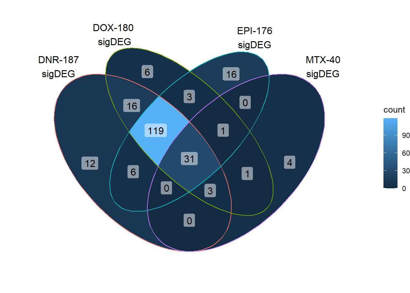 Here, I found 119 reQTLs that were related to all anthracyclines, with
31 reQTLS related to all Top2i drugs at 24 hours.
Here, I found 119 reQTLs that were related to all anthracyclines, with
31 reQTLS related to all Top2i drugs at 24 hours.
 DOXeQTL_table <- toplistall %>%
  mutate(sigcount = if_else(adj.P.Val < 0.05,'sig','notsig'))%>%
  mutate(DOXreQTLs=if_else(ENTREZID %in%DOXreQTLs$ENTREZID,"y","no")) %>%
  dplyr::filter(time =="24_hours") %>%
  dplyr::select(ENTREZID,id,DOXreQTLs,sigcount) %>%
  group_by(id,DOXreQTLs,sigcount) %>%
  tally() %>% as.data.frame() %>%
  pivot_wider(.,id_cols = c(id,DOXreQTLs),names_from = sigcount,values_from = n) %>%
  dplyr::select(id,DOXreQTLs,sig)
DOXeQTL_table%>%
  kable(., caption= "All 24 hour sigDEGs broken down by drug and DOXreQTL status") %>%
  kable_paper("striped", full_width = FALSE) %>%
  kable_styling(full_width = FALSE, position = "left",bootstrap_options = c("striped"),font_size = 18) %>%
scroll_box(width = "80%", height = "400px")| id | DOXreQTLs | sig |
|---|---|---|
| Daunorubicin | no | 6695 |
| Daunorubicin | y | 169 |
| Doxorubicin | no | 6336 |
| Doxorubicin | y | 180 |
| Epirubicin | no | 6048 |
| Epirubicin | y | 154 |
| Mitoxantrone | no | 1291 |
| Mitoxantrone | y | 36 |
| Trastuzumab | no | NA |
| Trastuzumab | y | NA |
DOXeQTL_table %>%
  add_row(id=c("Dox-specific DEGs","Dox-specific DEGs"),DOXreQTLs=c("no","y"), sig = c(62,1)) %>%
  dplyr::filter(DOXreQTLs=="y") %>%
  mutate(opp= 180-sig) %>%
  filter(id !=c('Trastuzumab','Doxorubicin')) %>%
  rename("yes"=sig, "no"=opp) %>%
  mutate(y_percent= paste0(sprintf("%2.1f", yes/(yes+no)*100), "%"),n_percent = paste0(sprintf("%2.1f", no/(yes+no)*100),"%")) %>%
  pivot_longer(!c(id,DOXreQTLs,y_percent,n_percent), names_to="group", values_to = "count") %>%
  mutate(id=factor(id, levels=c("Daunorubicin","Epirubicin", "Mitoxantrone","Dox-specific DEGs"))) %>%
ggplot(., aes(y=id,x=count,fill=group))+
     geom_col(position='fill')+
    theme_classic()+
   scale_color_manual(values=c("red4","navy"))+
    scale_fill_manual(values=c("#2297E6","red2"))+
  ggtitle("DOXreQTLs overlaps")+
  scale_y_discrete(limits=rev)+
  geom_text(aes(y=id,x=1, label = n_percent,hjust=.8))+

    theme(plot.title = element_text(size = rel(1.5), hjust = 0.5),
        axis.title = element_text(size = 15, color = "black"),
        axis.ticks = element_line(linewidth = 1.0),
        axis.line = element_line(linewidth = 1.0),
        axis.text = element_text(size = 10, color = "black", angle = 0),
        strip.text.x = element_text(size = 15, color = "black", face = "bold"))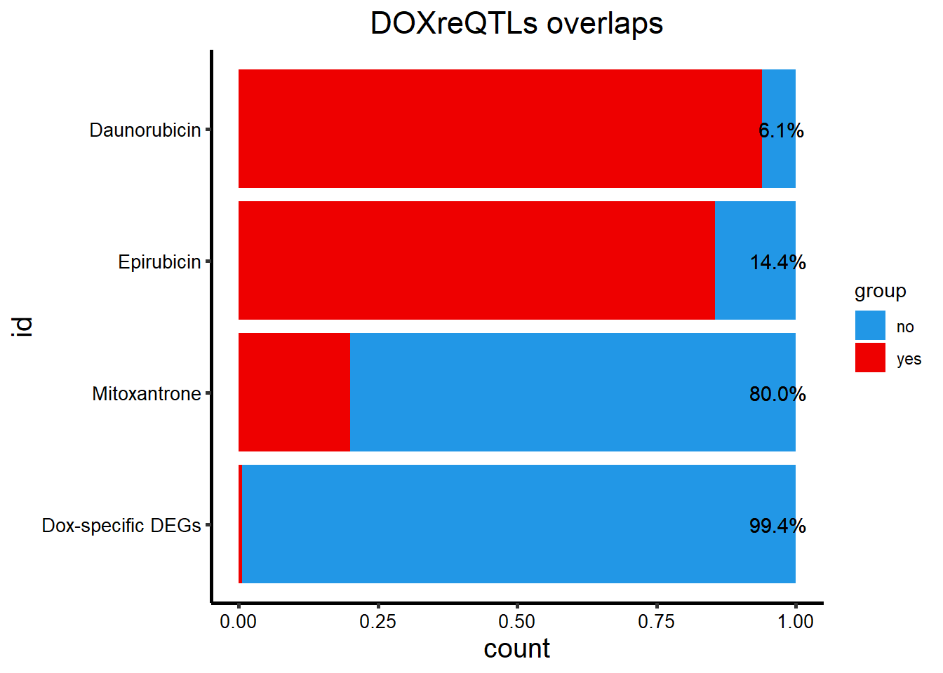
DOX specific-Dox dE-reqtl
DoxonlyQTL <- as.numeric(QTLoverlaps$..values..[[14]])
# geneDoxonlyQTL <- getBM(attributes=my_attributes,filters ='entrezgene_id',
# values =DoxonlyQTL, mart = ensembl)
# write.csv(geneDoxonlyQTL,"data/geneDoxonlyQTL.csv")
# saveRDS(cpmcounts,"data/cpmcount.RDS")
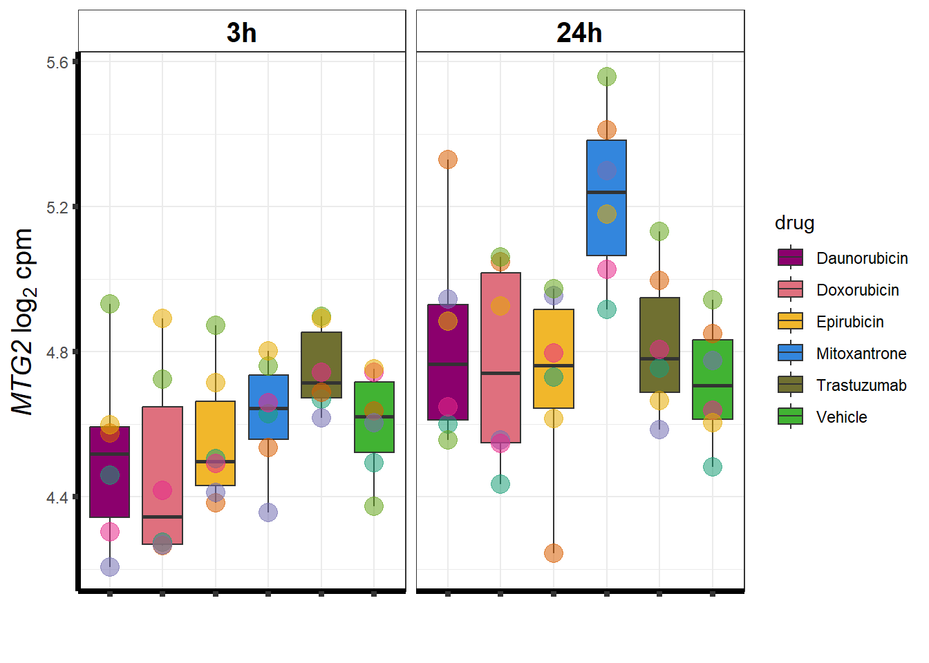
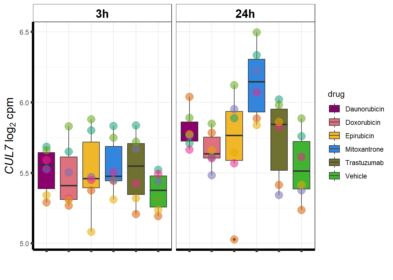
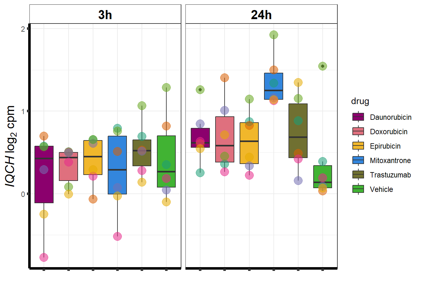
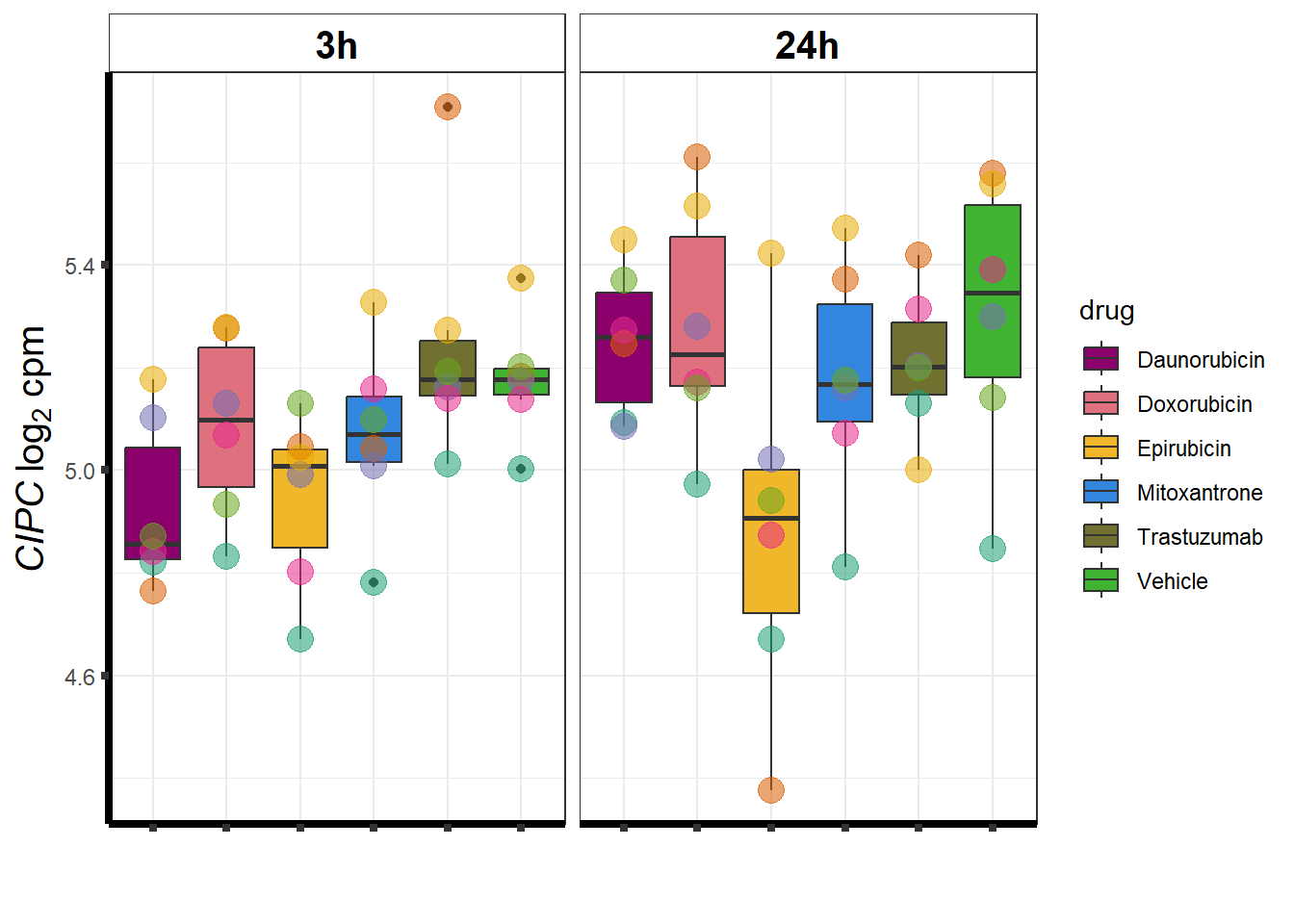
geneDoxonlyQTL <- read.csv("data/geneDoxonlyQTL.csv",row.names = 1)
cpmcounts <- readRDS("data/cpmcount.RDS")
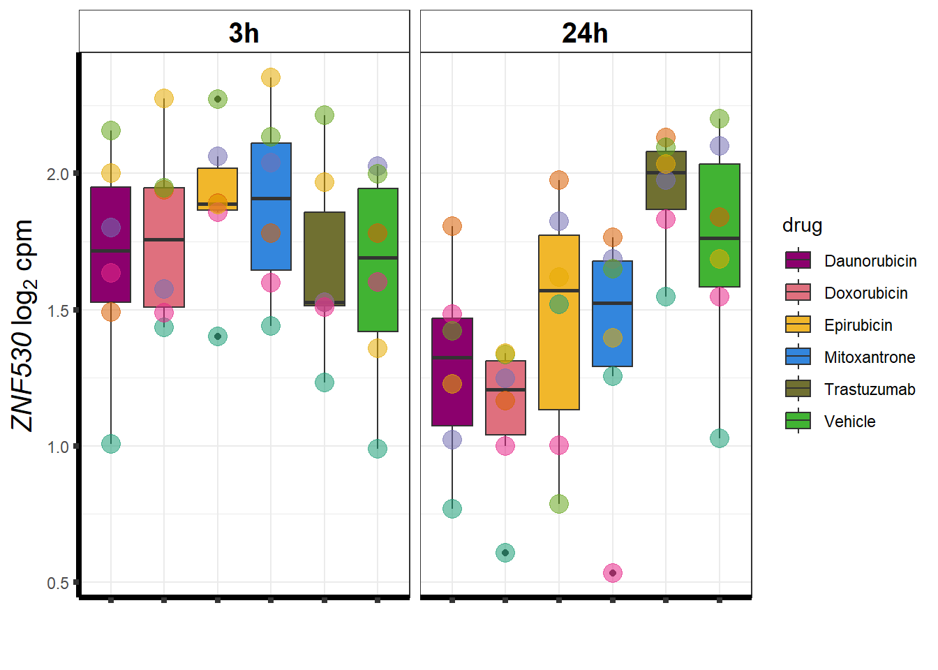
for (g in seq(from=1, to=length(geneDoxonlyQTL$entrezgene_id))){
a <- geneDoxonlyQTL$hgnc_symbol[g]
cpm_boxplot(cpmcounts,GOI=geneDoxonlyQTL[g,1],"Dark2",drug_palc,
ylab=bquote(~italic(.(a))~log[2]~"cpm "))
}
 ### Dox specific DEG examination
#pull list
total24 <-list(sigVDA24$ENTREZID,sigVDX24$ENTREZID,sigVEP24$ENTREZID,sigVMT24$ENTREZID)
## do venn partition and pull doxspe genes


venn_24h <- VennDiagram::get.venn.partitions(total24)
DoxonlyDEG <- venn_24h$..values..[[14]]
EpionlyDEG <- venn_24h$..values..[[12]]
DnronlyDEG <- venn_24h$..values..[[15]]
MtxonlyDEG <- venn_24h$..values..[[8]]


Dox24_lfc <- toplist24hr %>%
  filter(ENTREZID %in% DoxonlyDEG) %>%
  filter(adj.P.Val<0.05) %>%
  mutate(logFC=logFC*(-1)) %>%
  ggplot(., aes(x= id, y=logFC))+
  geom_boxplot(aes(fill=id))+
  theme_classic()+
  fill_palette(palette = drug_palNoVeh)+
  ggtitle("LogFC of Dox specific DEGs")+
  theme(
    plot.title = element_text(size = rel(1.5), hjust = 0.5,face = "bold"),
    axis.title = element_text(size = 15, color = "black"),
    axis.ticks = element_line(size = 1.5),
    axis.text = element_text(size = 8, color = "black", angle = 20))
    # strip.text.x = element_text(size = 12, color = "black", face = "italic"))

  toplist24hr %>%
  filter(ENTREZID %in% DoxonlyDEG) %>%
  filter(adj.P.Val<0.05) %>%
  ggplot(., aes(x=adj.P.Val))+
  geom_histogram(aes(fill=id,position="dodge"))+
    # geom_density(aes(fill=id))+
    facet_wrap(~id)+
    fill_palette(palette = drug_palNoVeh)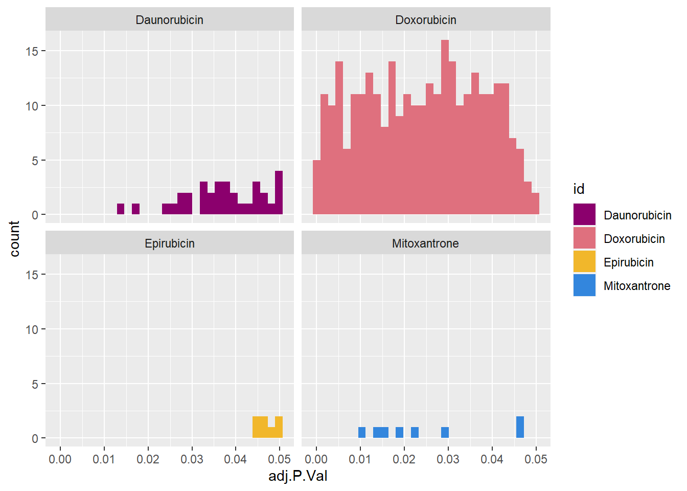
toplist24hr %>%
  filter(ENTREZID %in% DoxonlyDEG) %>%
  ggplot(., aes(x=adj.P.Val))+
  geom_density(aes(fill=id, alpha= 0.8))+
  fill_palette(palette = drug_palNoVeh)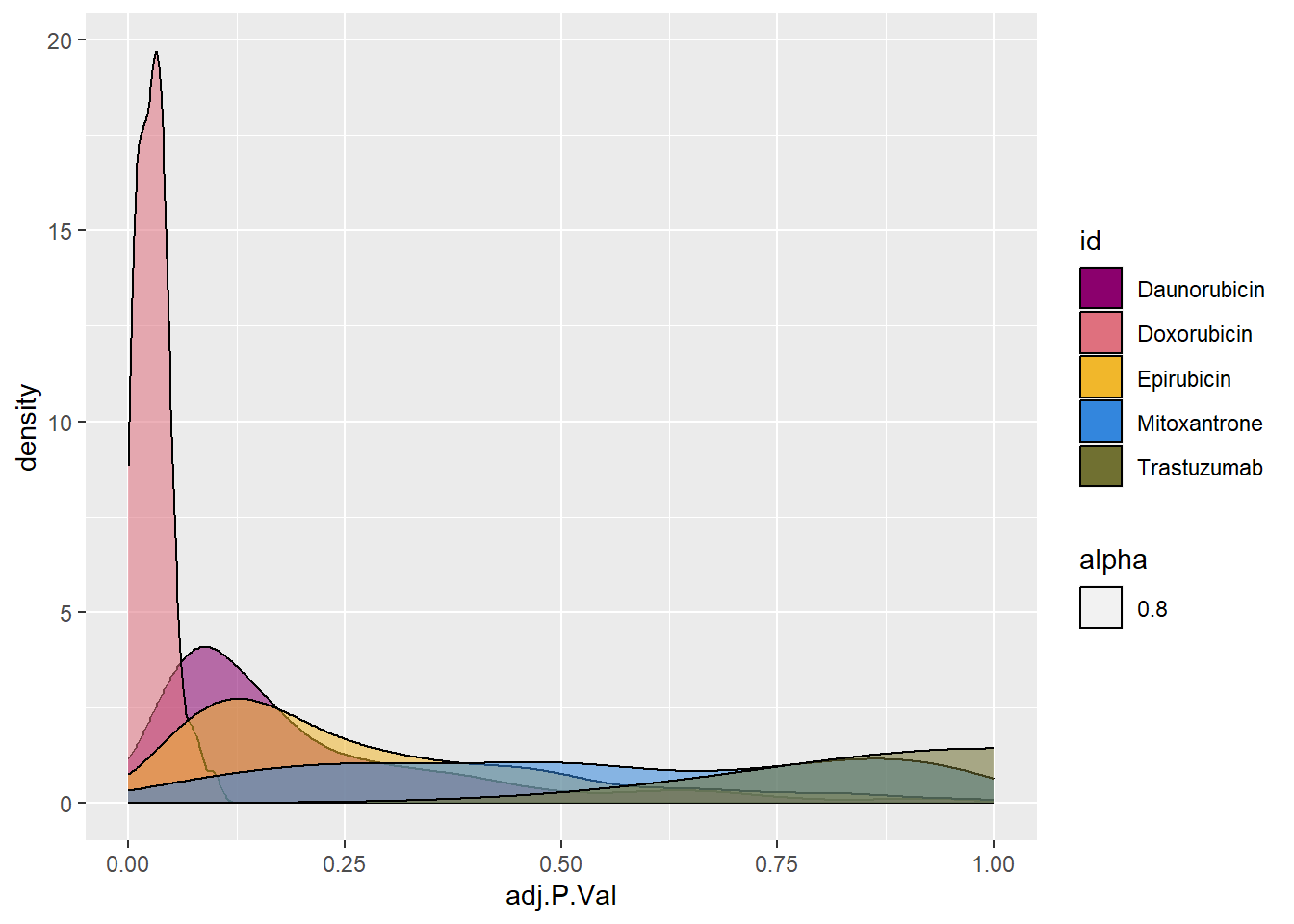
print(Dox24_lfc)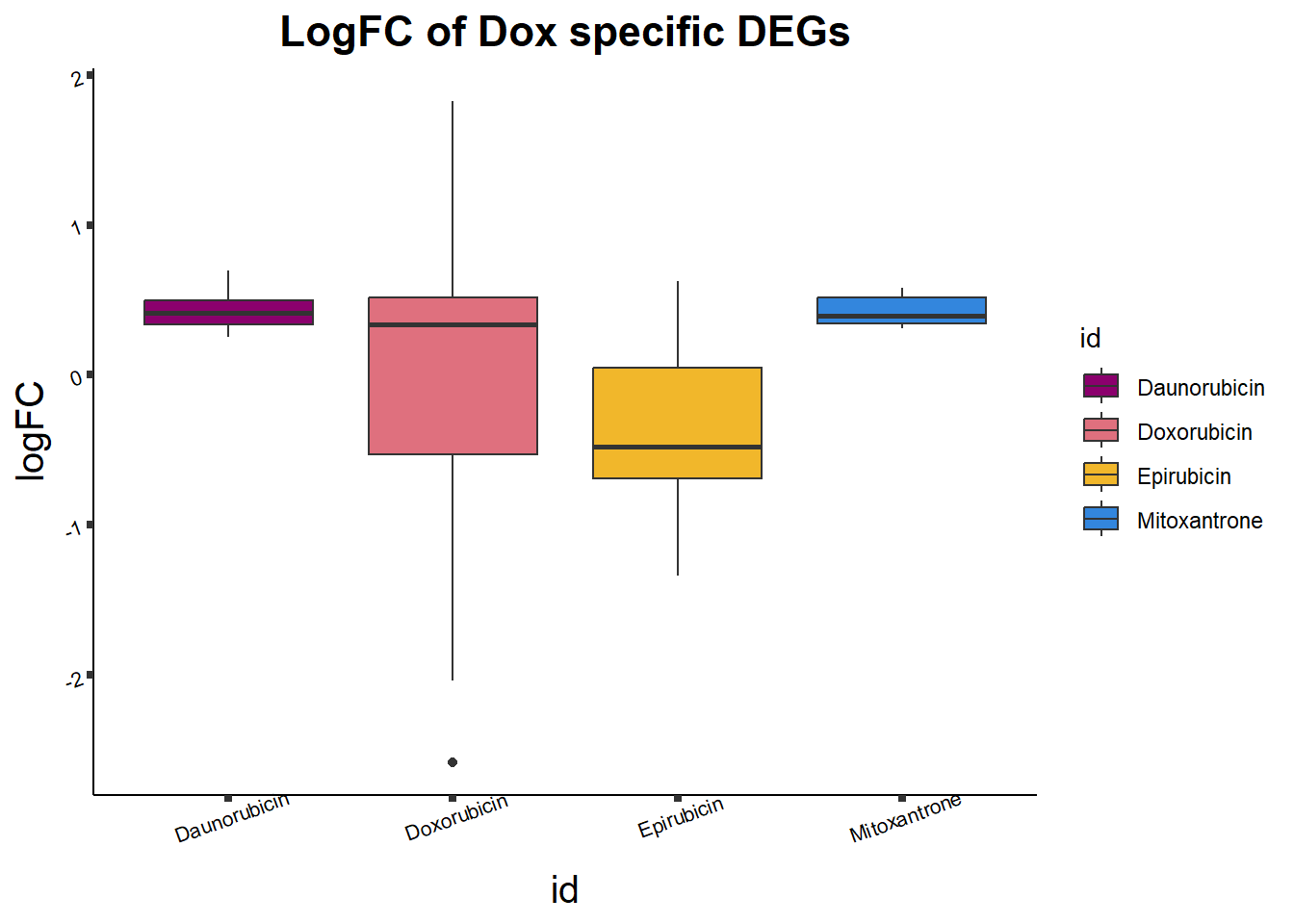
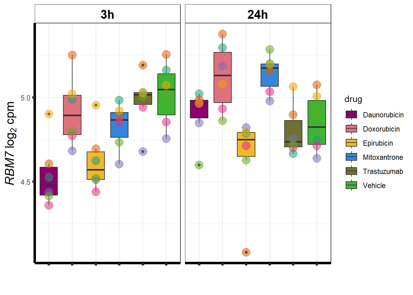
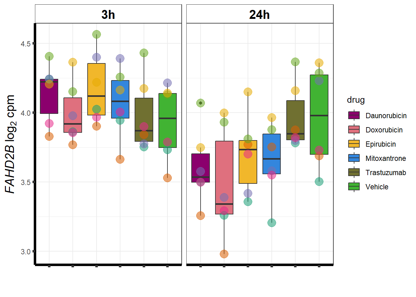
Plots of some genes:
### making list
#
# Doxonly_deg <- getBM(attributes=my_attributes,filters ='entrezgene_id',
#                   values =DoxonlyDEG, mart = ensembl)
# write.csv(Doxonly_deg,"output/Doxonly_deg.csv")
Doxonly_deg <- read.csv("output/Doxonly_deg.csv", row.names = 1)
set.seed(12345)
sampset <- Doxonly_deg %>%
  distinct(entrezgene_id,.keep_all = TRUE) %>%
  sample_n(.,12)
for (g in seq(from=1, to=length(sampset$entrezgene_id))){
  a <- sampset$hgnc_symbol[g]
  cpm_boxplot(cpmcounts,GOI=sampset[g,1],"Dark2",drug_palc,
                ylab=bquote(~italic(.(a))~log[2]~"cpm "))

}
More investigation of 24 hour specific genes
Doxorubicin
DOXdeg_sp <- toplist24hr %>%
  filter(if_else(id=="Doxorubicin",adj.P.Val<0.01,adj.P.Val>0.01 )) %>%
  filter(ENTREZID %in% DoxonlyDEG) %>%
  filter(id=="Doxorubicin") %>%
  dplyr::select(ENTREZID, SYMBOL)

DOXdeg_sp %>%
  kable(., caption= "DOX specific genes") %>%
  kable_paper("striped", full_width = TRUE) %>%
  kable_styling(full_width = FALSE, font_size = 16) %>%
scroll_box( height = "500px")| ENTREZID | SYMBOL | |
|---|---|---|
| 169200 | 169200 | TMEM64 |
| 653082 | 653082 | ZDHHC11B |
| 1452 | 1452 | CSNK1A1 |
| 23108 | 23108 | RAP1GAP2 |
| 114882 | 114882 | OSBPL8 |
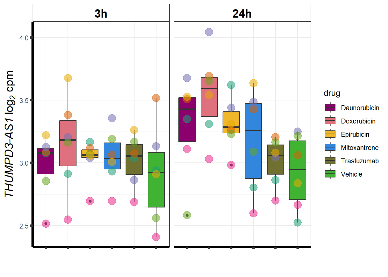
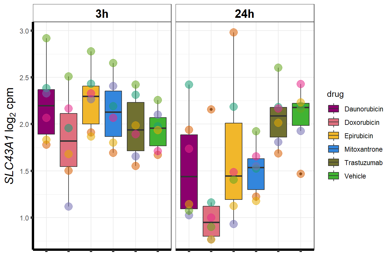
| 8501 | 8501 | SLC43A1 |
| 5000 | 5000 | ORC4 |
| 202181 | 202181 | LOC202181 |
| 135154 | 135154 | SDHAF4 |
| 122553 | 122553 | TRAPPC6B |
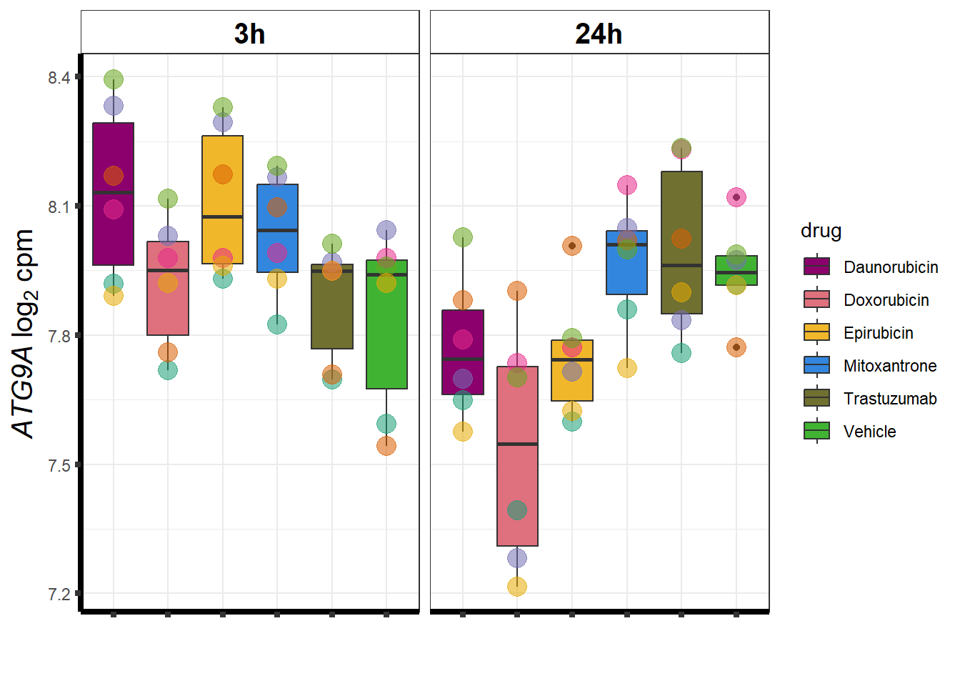
| 79065 | 79065 | ATG9A |
| 8763 | 8763 | CD164 |
| 284900 | 284900 | TTC28-AS1 |
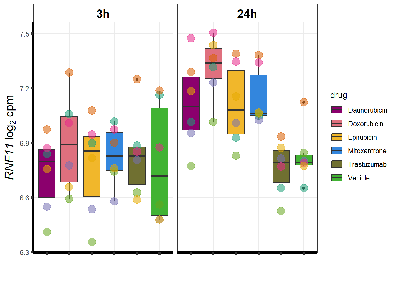
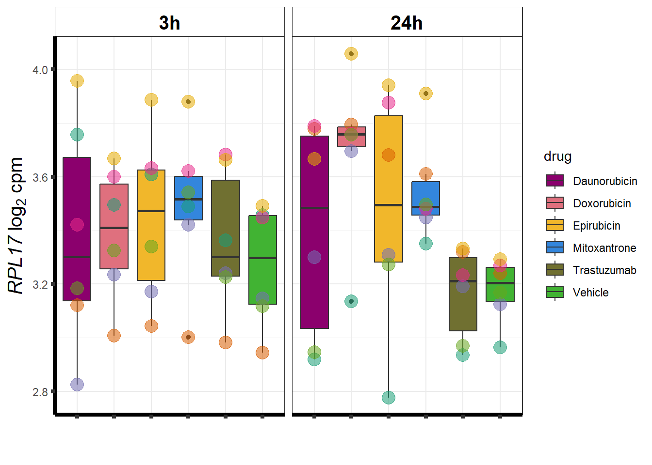
| 26994 | 26994 | RNF11 |
| 256586 | 256586 | LYSMD2 |
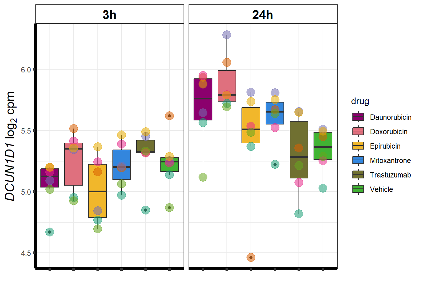
| 54165 | 54165 | DCUN1D1 |
| 8515 | 8515 | ITGA10 |
| 440944 | 440944 | THUMPD3-AS1 |
| 57181 | 57181 | SLC39A10 |
| 57338 | 57338 | JPH3 |
| 2230 | 2230 | FDX1 |
| 23548 | 23548 | TTC33 |
| 81532 | 81532 | MOB2 |
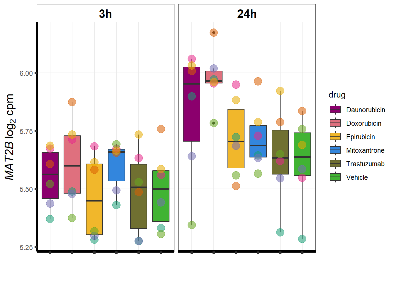
| 27430 | 27430 | MAT2B |
| 9524 | 9524 | TECR |
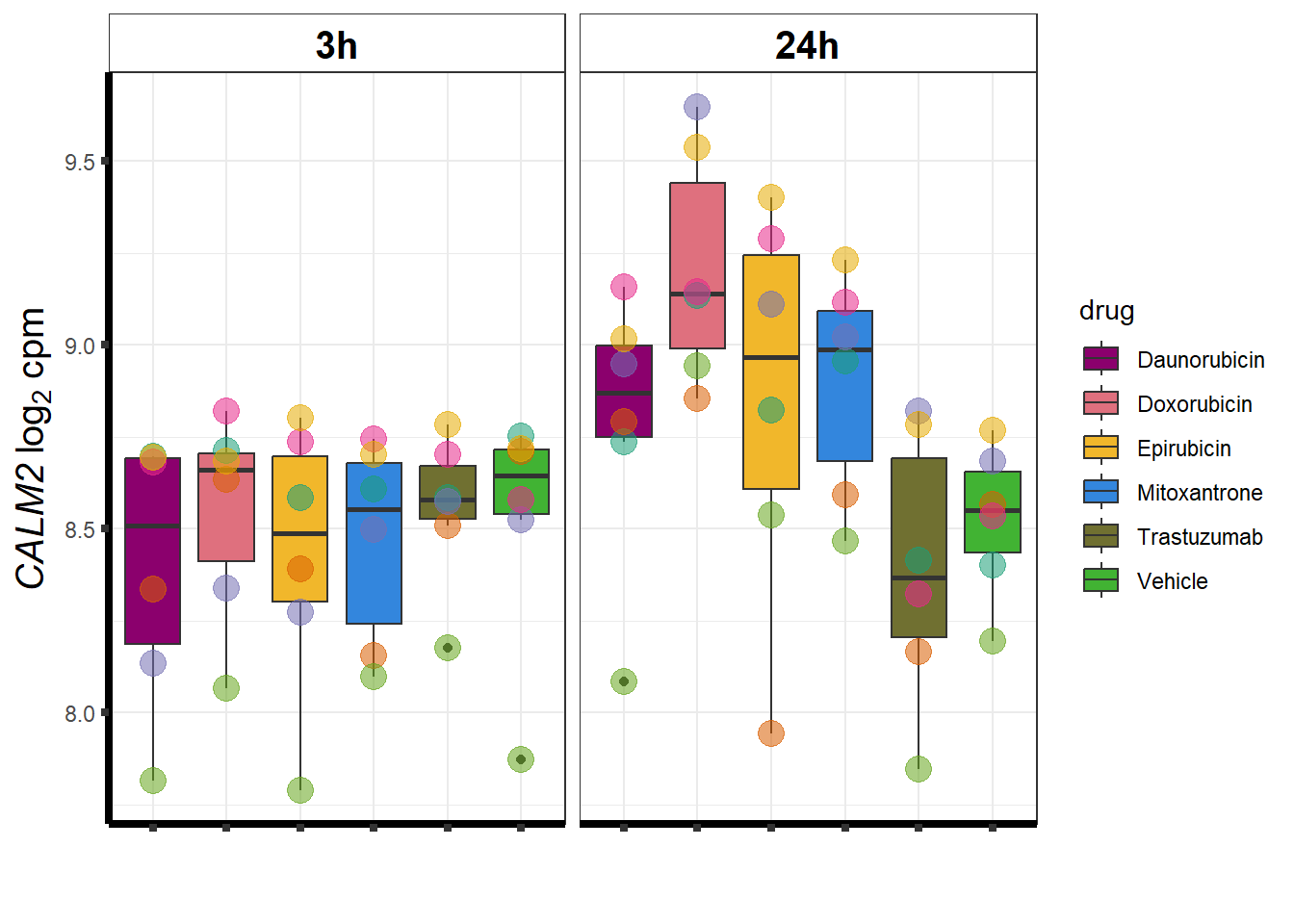
| 805 | 805 | CALM2 |
| 147 | 147 | ADRA1B |
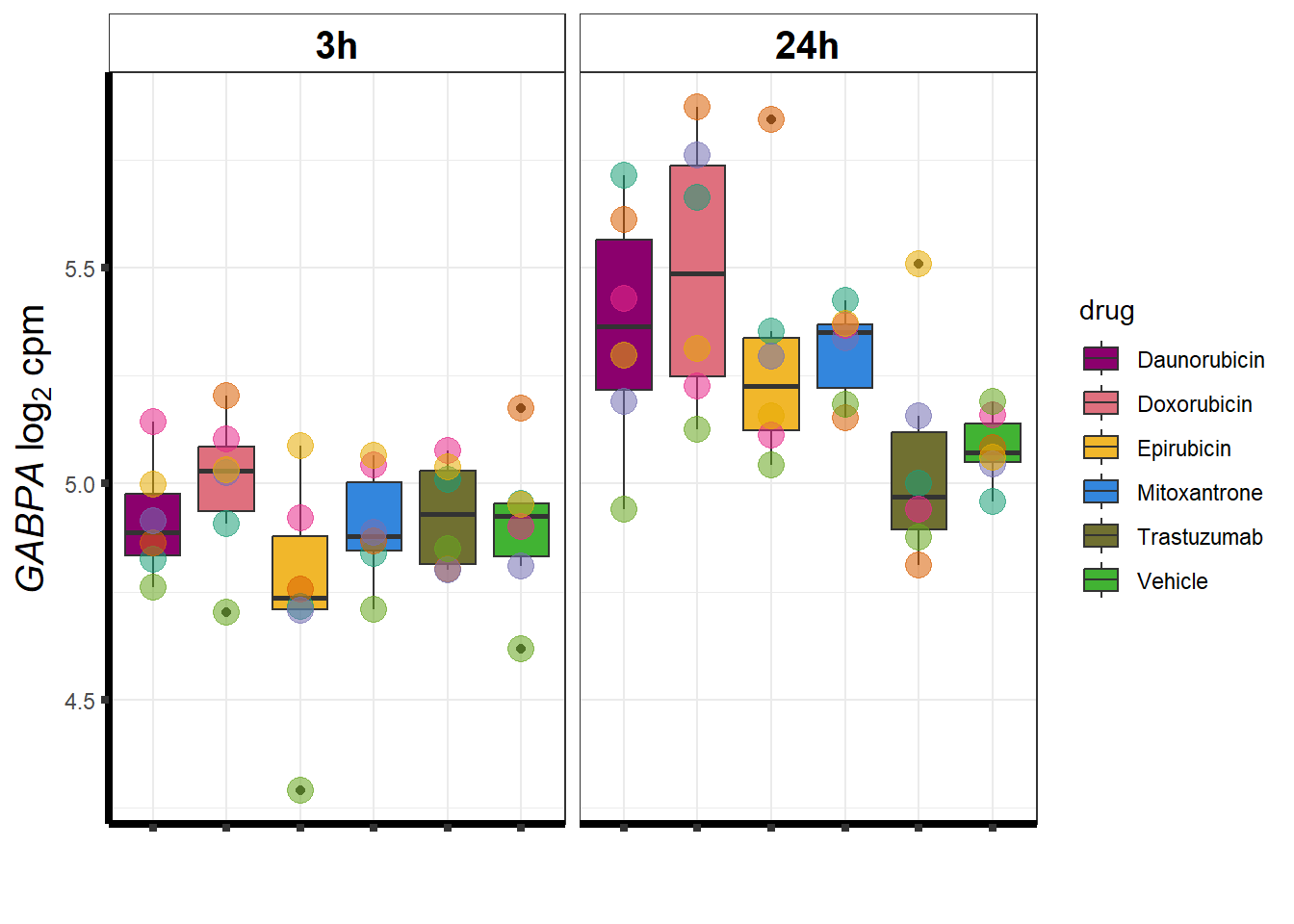
| 2551 | 2551 | GABPA |
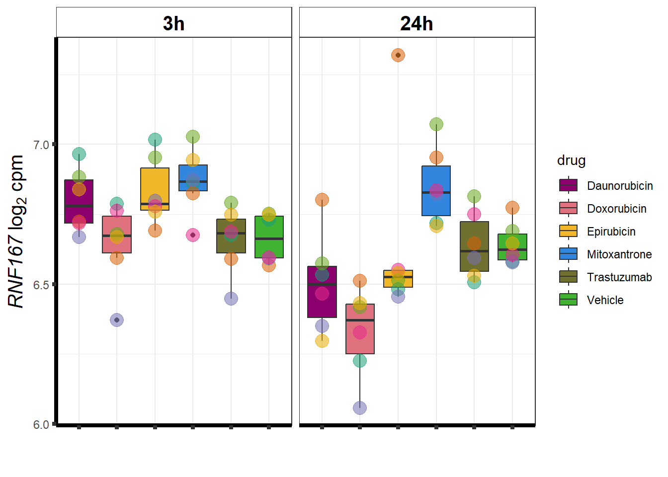
| 26001 | 26001 | RNF167 |
| 100131211 | 100131211 | NEMP2 |
| 79624 | 79624 | ARMT1 |
| 10190 | 10190 | TXNDC9 |
| 7917 | 7917 | BAG6 |
| 6653 | 6653 | SORL1 |
| 9039 | 9039 | UBA3 |
| 57862 | 57862 | ZNF410 |
| 6498 | 6498 | SKIL |
| 112858 | 112858 | TP53RK |
| 101927720 | 101927720 | ZNF793-AS1 |
| 56998 | 56998 | CTNNBIP1 |
| 5431 | 5431 | POLR2B |
| 25842 | 25842 | ASF1A |
| 55664 | 55664 | CDC37L1 |
| 57186 | 57186 | RALGAPA2 |
| 5598 | 5598 | MAPK7 |
| 5594 | 5594 | MAPK1 |
| 58490 | 58490 | RPRD1B |
| 8848 | 8848 | TSC22D1 |
| 29944 | 29944 | PNMA3 |
| 2130 | 2130 | EWSR1 |
| 6139 | 6139 | RPL17 |
| 9446 | 9446 | GSTO1 |
| 102723508 | 102723508 | KANTR |
| 4987 | 4987 | OPRL1 |
| 84458 | 84458 | LCOR |
| 84752 | 84752 | B3GNT9 |
| 54629 | 54629 | MINDY2 |
| 54469 | 54469 | ZFAND6 |
| 144363 | 144363 | ETFRF1 |
| 9821 | 9821 | RB1CC1 |
| 116068 | 116068 | LYSMD3 |
| 66036 | 66036 | MTMR9 |
intersect(DOXreQTLs$ENTREZID, DOXdeg_sp$ENTREZID)[1] "57338"toplist24hr %>%
group_by(time,id) %>%
filter(ENTREZID %in% DOXdeg_sp$ENTREZID) %>%
filter(adj.P.Val <0.05) %>%
# filter(id=="Doxorubicin")
mutate(logFC=logFC*(-1)) %>%
ggplot(., aes(x= id, y=logFC))+
geom_boxplot(aes(fill=id))+
theme_classic()+
fill_palette(palette = drug_palNoVeh)+
ggtitle("LogFC of n=62 Dox specific DEGs")+
theme(
plot.title = element_text(size = rel(1.5), hjust = 0.5,face = "bold"),
axis.title = element_text(size = 15, color = "black"),
axis.ticks = element_line(size = 1.5),
axis.text = element_text(size = 8, color = "black", angle = 20))
    # strip.text.x = element_text(size = 12, color = "black", face = "italic"))

toplist24hr %>% group_by(time,id) %>%
  filter(ENTREZID %in% DoxonlyDEG) %>%
  filter(adj.P.Val <0.05) %>%
  ggplot(., aes(x=adj.P.Val))+
  geom_histogram(aes(fill=id))+
  geom_vline(xintercept=0.01,linetype=2)+
    # geom_density(aes(fill=id))+
    facet_wrap(~id)+
  ggtitle("all DE-DOX adj p. value <0.05")+
    fill_palette(palette = drug_palNoVeh)+
  theme_bw()
toplist24hr %>%
  filter(if_else(id=="Doxorubicin",adj.P.Val<0.01,adj.P.Val>0.01 )) %>%
  group_by(time,id) %>%
  filter(ENTREZID %in% DOXdeg_sp$ENTREZID) %>%
  filter(adj.P.Val <0.05) %>%
  ggplot(., aes(x=adj.P.Val))+
  geom_histogram(aes(fill=id))+
  geom_vline(xintercept=0.01,linetype=2)+
    # geom_density(aes(fill=id))+
    facet_wrap(~id)+
  ggtitle("all Dox specific DEG adj p. value <0.01")+
    fill_palette(palette = drug_palNoVeh)+
  theme_bw()
toplist24hr %>%
  filter(ENTREZID %in% DoxonlyDEG) %>%
  # filter(adj.P.Val<0.05) %>%
  ggplot(., aes(x=adj.P.Val))+
  geom_density(aes(fill=id, alpha= 0.8))+
  fill_palette(palette = drug_palNoVeh)+
  theme_bw()
toplist24hr %>%
  filter(ENTREZID %in% DOXdeg_sp$ENTREZID) %>%
  # filter(adj.P.Val<0.05) %>%
  ggplot(., aes(x=adj.P.Val))+
  geom_density(aes(fill=id, alpha= 0.8))+
  fill_palette(palette = drug_palNoVeh)+
  theme_bw()
set.seed(12345)
sampset <- DOXdeg_sp %>%
  sample_n(.,12)

for (g in seq(from=1, to=length(sampset$ENTREZID))){
  a <- sampset$SYMBOL[g]
  cpm_boxplot(cpmcounts,GOI=sampset[g,1],"Dark2",drug_palc,
                ylab=bquote(~italic(.(a))~log[2]~"cpm "))
}
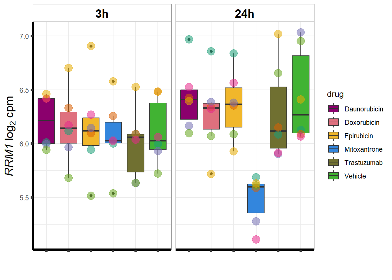
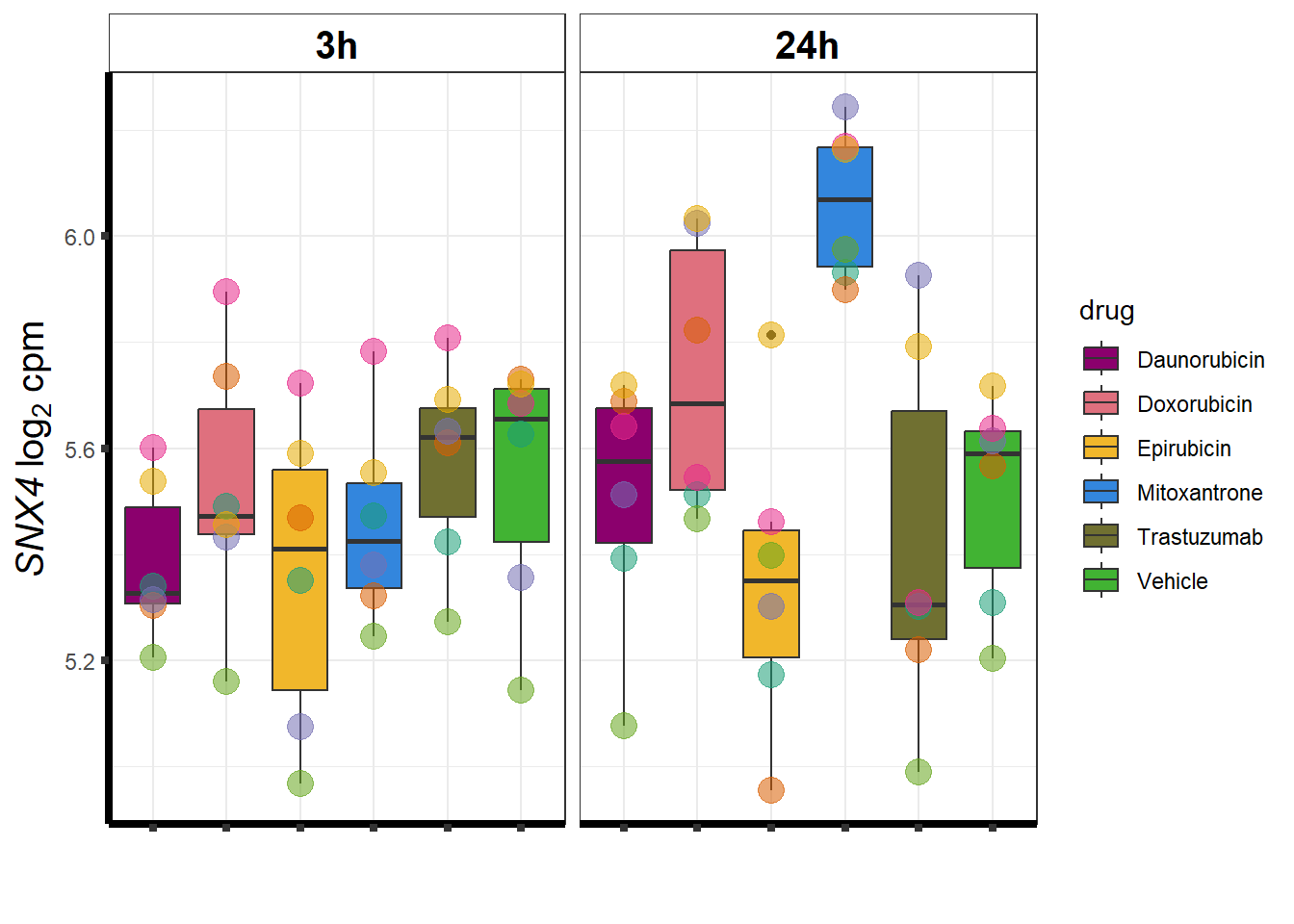
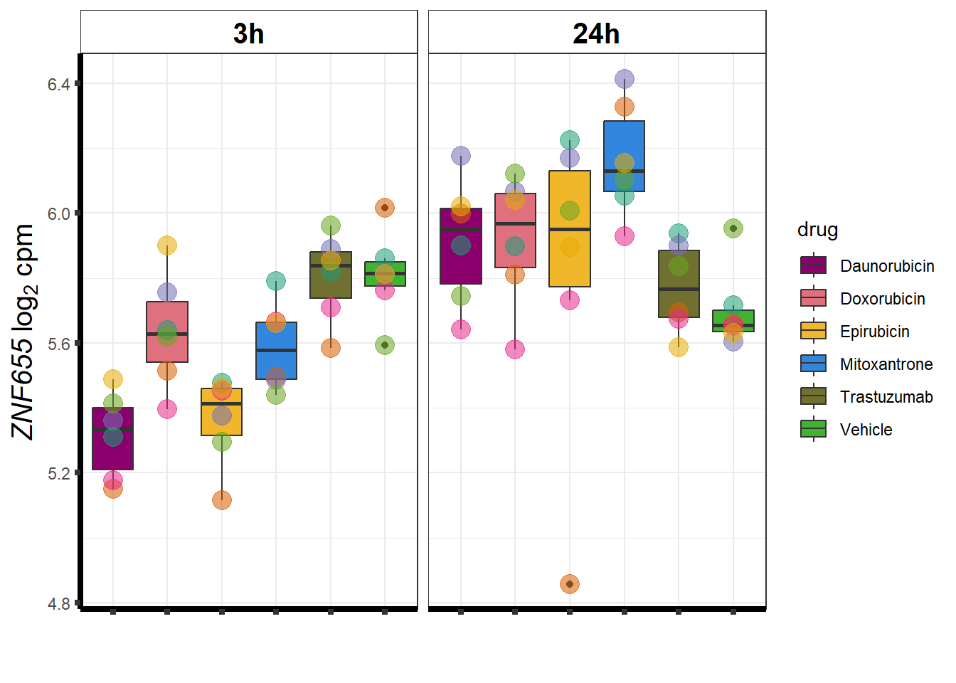
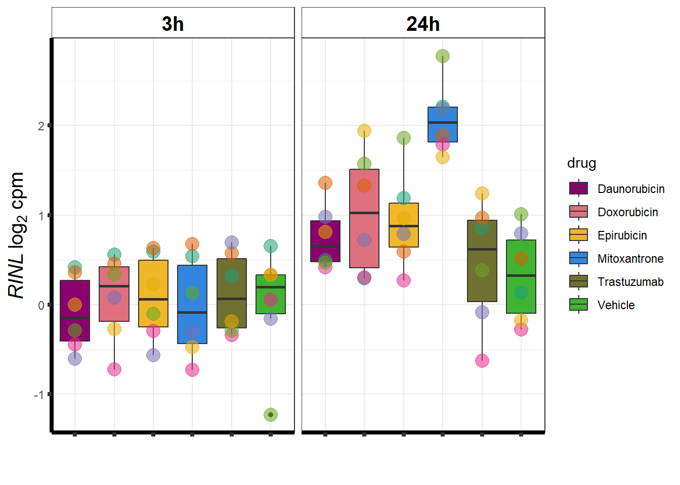
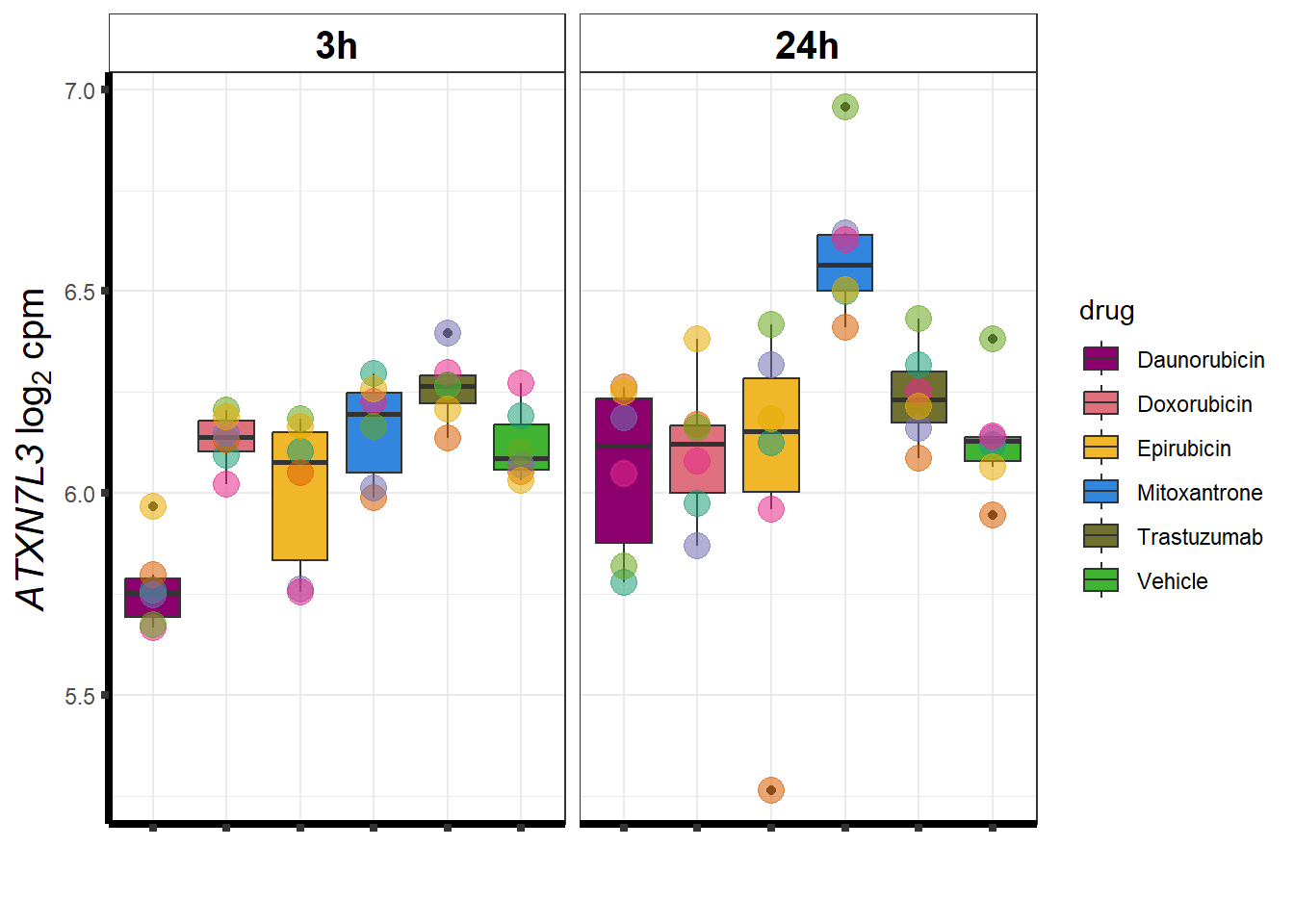
 ### Mitoxantrone
MTXdeg_sp <- toplist24hr %>%
  filter(if_else(id=="Mitoxantrone",adj.P.Val<0.01,adj.P.Val>0.01 )) %>%
  filter(ENTREZID %in% MtxonlyDEG) %>%
  filter(id=="Mitoxantrone") %>%
  dplyr::select(ENTREZID, SYMBOL)

MTXdeg_sp %>%
  kable(., caption= "MTX specific genes") %>%
  kable_paper("striped", full_width = TRUE) %>%
  kable_styling(full_width = FALSE, font_size = 16) %>%
scroll_box( height = "500px")| ENTREZID | SYMBOL | |
|---|---|---|
| 25894 | 25894 | PLEKHG4 |
| 126432 | 126432 | RINL |
| 100128191 | 100128191 | TMPO-AS1 |
| 63827 | 63827 | BCAN |
| 55147 | 55147 | RBM23 |
| 253714 | 253714 | MMS22L |
| 23582 | 23582 | CCNDBP1 |
| 4077 | 4077 | NBR1 |
| 7014 | 7014 | TERF2 |
| 25886 | 25886 | POC1A |
| 6240 | 6240 | RRM1 |
| 83879 | 83879 | CDCA7 |
| 79758 | 79758 | DHRS12 |
| 23786 | 23786 | BCL2L13 |
| 55723 | 55723 | ASF1B |
| 22950 | 22950 | SLC4A1AP |
| 54853 | 54853 | WDR55 |
| 4001 | 4001 | LMNB1 |
| 100996573 | 100996573 | NA |
| 55780 | 55780 | ERMARD |
| 25981 | 25981 | DNAH1 |
| 56970 | 56970 | ATXN7L3 |
| 11152 | 11152 | WDR45 |
| 9820 | 9820 | CUL7 |
| 23558 | 23558 | WBP2 |
| 6293 | 6293 | VPS52 |
| 150962 | 150962 | PUS10 |
| 26164 | 26164 | MTG2 |
| 64799 | 64799 | IQCH |
| 27346 | 27346 | TMEM97 |
| 55717 | 55717 | WDR11 |
| 8723 | 8723 | SNX4 |
| 4173 | 4173 | MCM4 |
| 10432 | 10432 | RBM14 |
| 655 | 655 | BMP7 |
| 9391 | 9391 | CIAO1 |
| 3148 | 3148 | HMGB2 |
| 8317 | 8317 | CDC7 |
| 441478 | 441478 | NRARP |
| 90120 | 90120 | TMEM250 |
| 57699 | 57699 | CPNE5 |
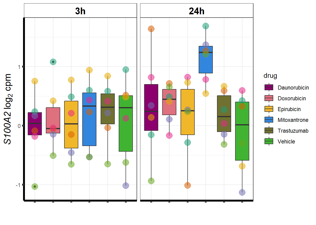
| 6273 | 6273 | S100A2 |
| 55670 | 55670 | PEX26 |
| 79027 | 79027 | ZNF655 |
| 11176 | 11176 | BAZ2A |
| 100131067 | 100131067 | CKMT2-AS1 |
| 84892 | 84892 | POMGNT2 |
| 9134 | 9134 | CCNE2 |
toplist24hr %>%
  filter(ENTREZID %in% MTXdeg_sp$ENTREZID) %>%
  filter(adj.P.Val <0.05) %>%
  # filter(id=="Mitoxantrone")
  mutate(logFC=logFC*(-1)) %>%
  add_row(time="24_hours",id="Epirubicin") %>%
  add_row(time="24_hours",id="Daunorubicin") %>%
  mutate(id= factor(id,levels= c("Daunorubicin", "Doxorubicin", "Epirubicin", "Mitoxantrone"))) %>%
  ggplot(., aes(x= id, y=logFC))+
  geom_boxplot(aes(fill=id))+
  theme_classic()+
  fill_palette(palette = drug_palNoVeh,drop = FALSE)+
  ggtitle("LogFC of n=48 MTX specific DEGs")+
  theme(
    plot.title = element_text(size = rel(1.5), hjust = 0.5,face = "bold"),
    axis.title = element_text(size = 15, color = "black"),
    axis.ticks = element_line(size = 1.5),
    axis.text = element_text(size = 8, color = "black", angle = 20))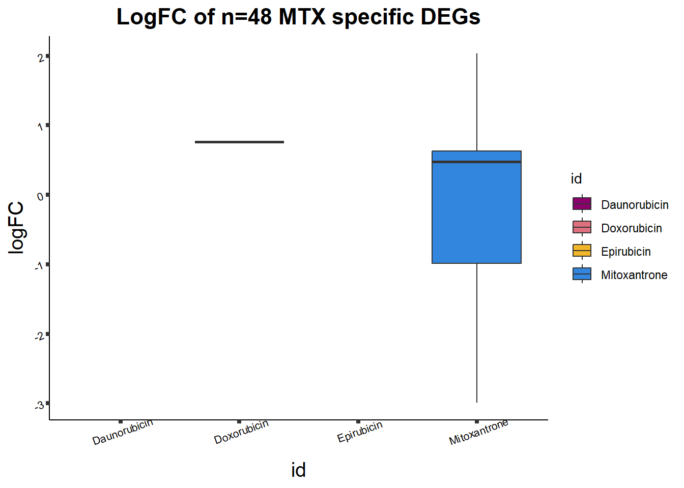
    # strip.text.x = element_text(size = 12, color = "black", face = "italic"))

toplist24hr %>%
  filter(if_else(id=="Mitoxantrone",adj.P.Val<0.01,adj.P.Val>0.01 )) %>%
  filter(ENTREZID %in% MtxonlyDEG) %>%
  filter(adj.P.Val <0.05) %>%
   add_row(time="24_hours",id="Epirubicin") %>%
   mutate(id= factor(id, levels = c("Daunorubicin", "Doxorubicin", "Epirubicin", "Mitoxantrone"))) %>%
   ggplot(., aes(x=adj.P.Val))+
  geom_histogram(aes(fill=id))+
  geom_vline(xintercept=0.01, linetype=2)+
    # geom_density(aes(fill=id))+
    facet_wrap(~id)+
  ggtitle("MTX adj p. value <0.05")+
    fill_palette(palette = drug_palNoVeh, drop = FALSE)+
  theme_bw()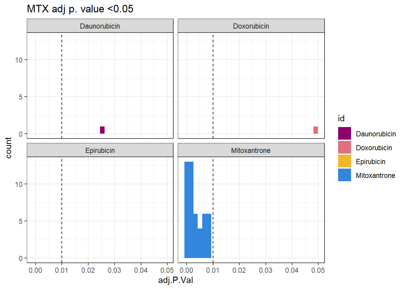
toplist24hr %>%
  # filter(if_else(id=="Mitoxantrone",adj.P.Val<0.01,adj.P.Val>0.01 )) %>%
  filter(ENTREZID %in% MtxonlyDEG) %>%
  filter(adj.P.Val <0.05) %>%
   add_row(time="24_hours",id="Epirubicin") %>%
   mutate(id= factor(id, levels = c("Daunorubicin", "Doxorubicin", "Epirubicin", "Mitoxantrone"))) %>%
   ggplot(., aes(x=adj.P.Val))+
  geom_histogram(aes(fill=id))+
  geom_vline(xintercept=0.01, linetype=2)+
    # geom_density(aes(fill=id))+
    facet_wrap(~id)+
  ggtitle("MTX adj p. value <0.05")+
    fill_palette(palette = drug_palNoVeh, drop = FALSE)+
  theme_bw()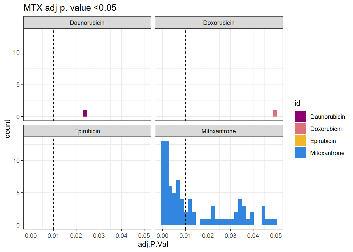
toplist24hr %>%
  filter(ENTREZID %in% MtxonlyDEG) %>%
  # filter(adj.P.Val<0.05) %>%
  ggplot(., aes(x=adj.P.Val))+
  geom_density(aes(fill=id, alpha= 0.8))+
  fill_palette(palette = drug_palNoVeh)+
  theme_bw()+
   ggtitle("All sigDE (adj.P.val <0.05) MTX genes")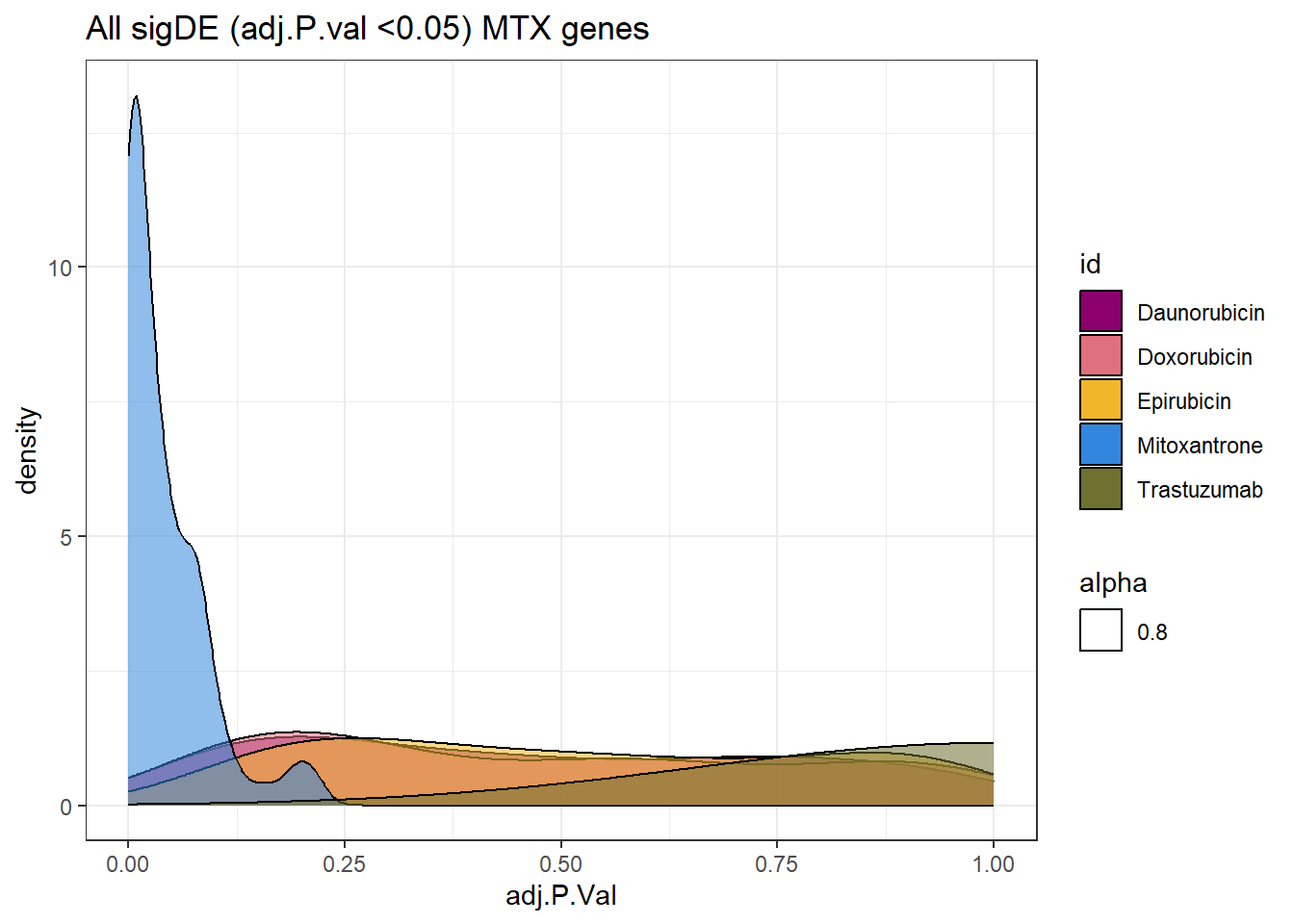
toplist24hr %>%
  filter(ENTREZID %in% MTXdeg_sp$ENTREZID) %>%
  # filter(adj.P.Val<0.05) %>%
  ggplot(., aes(x=adj.P.Val))+
  geom_density(aes(fill=id, alpha= 0.8))+
  fill_palette(palette = drug_palNoVeh)+
  theme_bw()+
  ggtitle("Only MTX specific (n=48) genes across all treatments")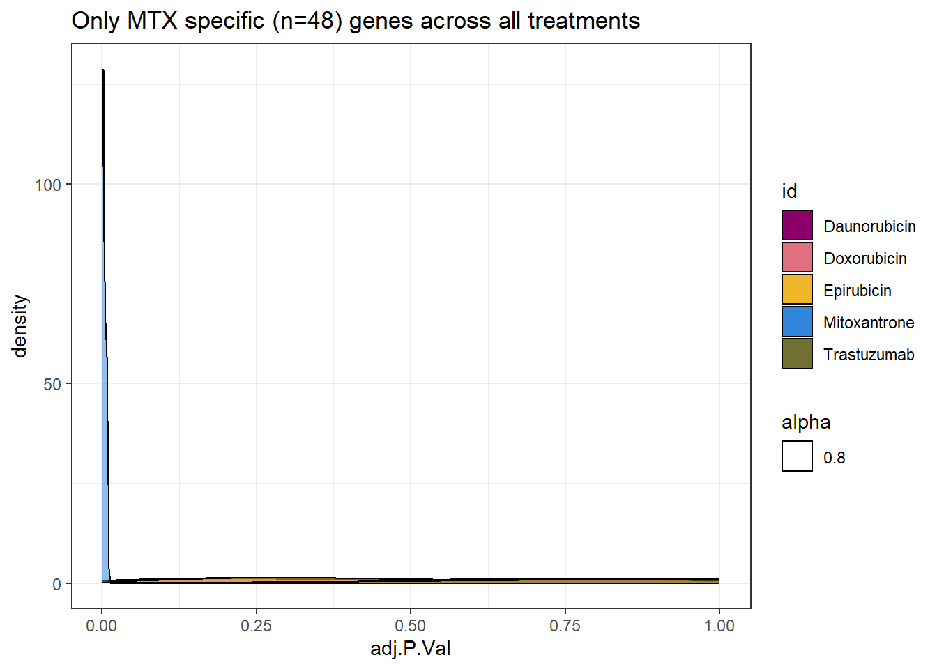
set.seed(12345)
sampset <- MTXdeg_sp %>%
sample_n(.,12)
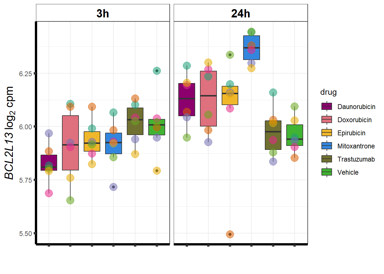
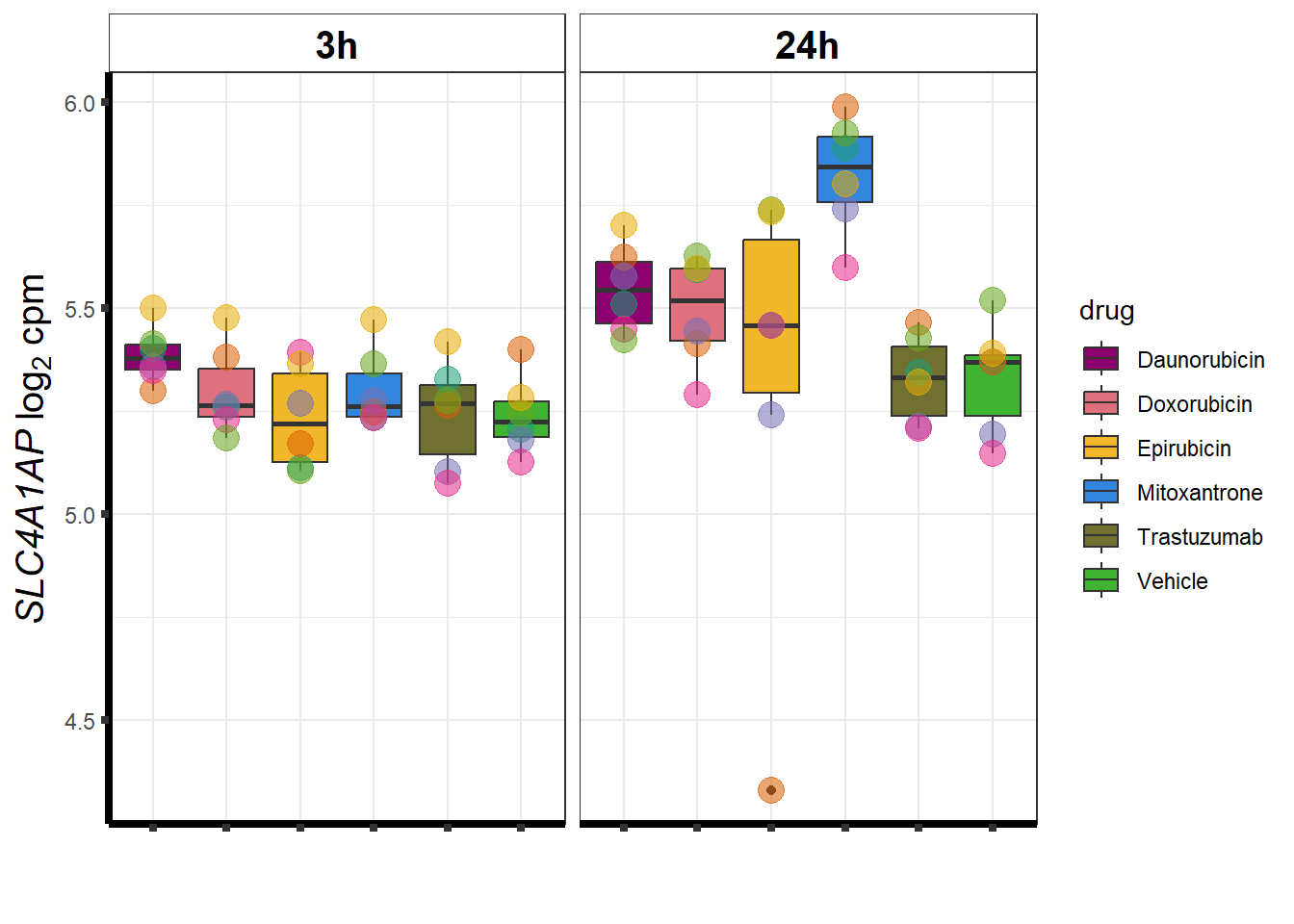
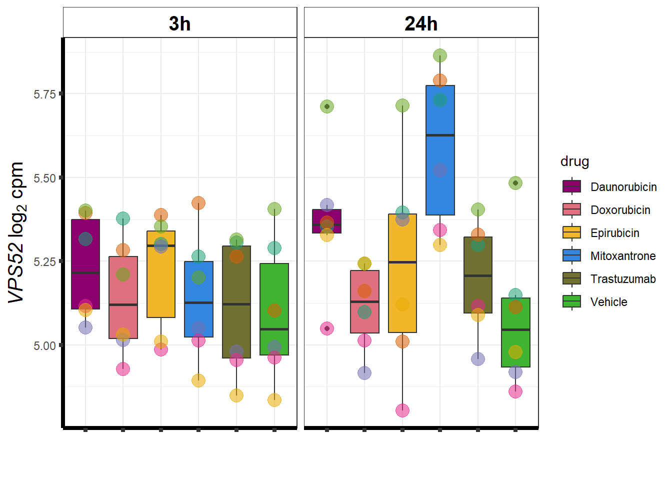
for (g in seq(from=1, to=length(sampset$ENTREZID))){
a <- sampset$SYMBOL[g]
cpm_boxplot(cpmcounts,GOI=sampset[g,1],"Dark2",drug_palc,
ylab=bquote(~italic(.(a))~log[2]~"cpm "))
}
Daunorubicin
DNRdeg_sp <- toplist24hr %>%
  filter(if_else(id=="Daunorubicin",adj.P.Val<0.01,adj.P.Val>0.01 )) %>%
  filter(ENTREZID %in% DnronlyDEG) %>%
  filter(id=="Daunorubicin") %>%
  dplyr::select(ENTREZID, SYMBOL)

DNRdeg_sp %>%
  kable(., caption= "DNR specific genes") %>%
  kable_paper("striped", full_width = TRUE) %>%
  kable_styling(full_width = FALSE, font_size = 16) %>%
scroll_box( height = "500px")| ENTREZID | SYMBOL | |
|---|---|---|
| 5742 | 5742 | PTGS1 |
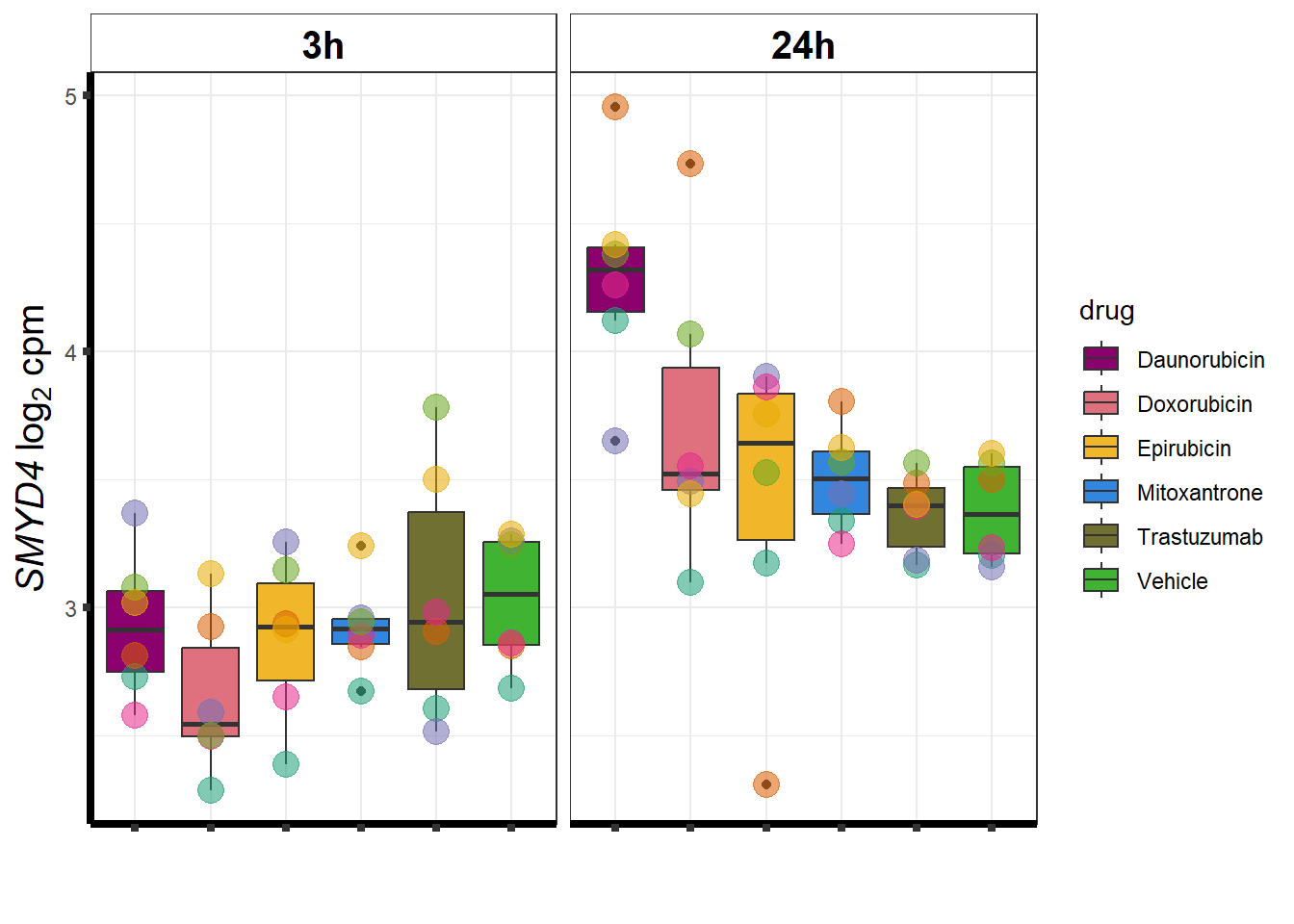
| 114826 | 114826 | SMYD4 |
| 6117 | 6117 | RPA1 |
| 54550 | 54550 | NECAB2 |
| 55000 | 55000 | TUG1 |
| 23150 | 23150 | FRMD4B |
| 128637 | 128637 | TBC1D20 |
| 8864 | 8864 | PER2 |
| 132430 | 132430 | PABPC4L |
| 54973 | 54973 | INTS11 |
| 140465 | 140465 | MYL6B |
| 81628 | 81628 | TSC22D4 |
| 53838 | 53838 | C11orf24 |
| 387640 | 387640 | SKIDA1 |
| 57654 | 57654 | UVSSA |
| 11273 | 11273 | ATXN2L |
| 56624 | 56624 | ASAH2 |
| 255043 | 255043 | TMEM86B |
| 23428 | 23428 | SLC7A8 |
| 4007 | 4007 | PRICKLE3 |
| 5915 | 5915 | RARB |
| 79137 | 79137 | RETREG2 |
| 57605 | 57605 | PITPNM2 |
| 4241 | 4241 | MELTF |
| 10043 | 10043 | TOM1 |
| 8766 | 8766 | RAB11A |
| 10233 | 10233 | LRRC23 |
| 23140 | 23140 | ZZEF1 |
| 7675 | 7675 | ZNF121 |
| 83606 | 83606 | GUCD1 |
| 6726 | 6726 | SRP9 |
| 5026 | 5026 | P2RX5 |
| 6550 | 6550 | SLC9A3 |
| 10457 | 10457 | GPNMB |
| 22982 | 22982 | DIP2C |
| 1200 | 1200 | TPP1 |
| 84922 | 84922 | FIZ1 |
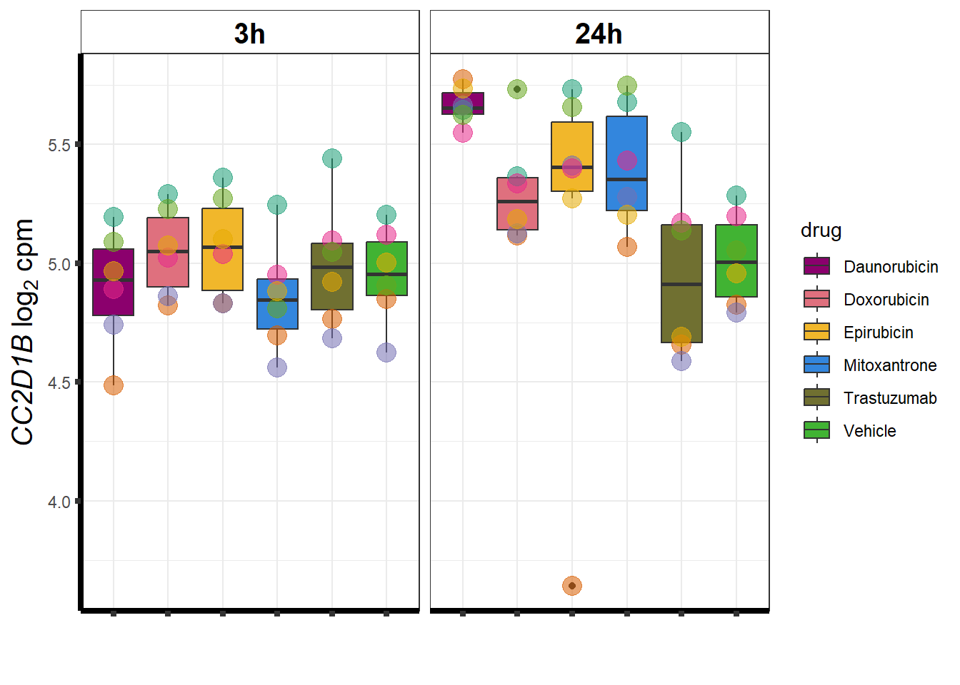
| 200014 | 200014 | CC2D1B |
| 4149 | 4149 | MAX |
| 55818 | 55818 | KDM3A |
| 3710 | 3710 | ITPR3 |
| 5350 | 5350 | PLN |
| 22938 | 22938 | SNW1 |
| 284612 | 284612 | SYPL2 |
| 10992 | 10992 | SF3B2 |
| 5463 | 5463 | POU6F1 |
| 9757 | 9757 | KMT2B |
| 146880 | 146880 | ARHGAP27P1 |
| 1827 | 1827 | RCAN1 |
| 29763 | 29763 | PACSIN3 |
| 10081 | 10081 | PDCD7 |
| 56132 | 56132 | PCDHB3 |
| 257144 | 257144 | GCSAM |
| 9929 | 9929 | JOSD1 |
| 7052 | 7052 | TGM2 |
| 11190 | 11190 | CEP250 |
| 388722 | 388722 | C1orf53 |
| 2188 | 2188 | FANCF |
| 375690 | 375690 | WASH5P |
| 28957 | 28957 | MRPS28 |
| 644150 | 644150 | WIPF3 |
| 4861 | 4861 | NPAS1 |
| 55876 | 55876 | GSDMB |
| 6832 | 6832 | SUPV3L1 |
| 90993 | 90993 | CREB3L1 |
| 64761 | 64761 | PARP12 |
| 7249 | 7249 | TSC2 |
| 158431 | 158431 | ZNF782 |
| 10580 | 10580 | SORBS1 |
| 220869 | 220869 | CBWD5 |
| 55140 | 55140 | ELP3 |
| 5587 | 5587 | PRKD1 |
| 80347 | 80347 | COASY |
| 6302 | 6302 | TSPAN31 |
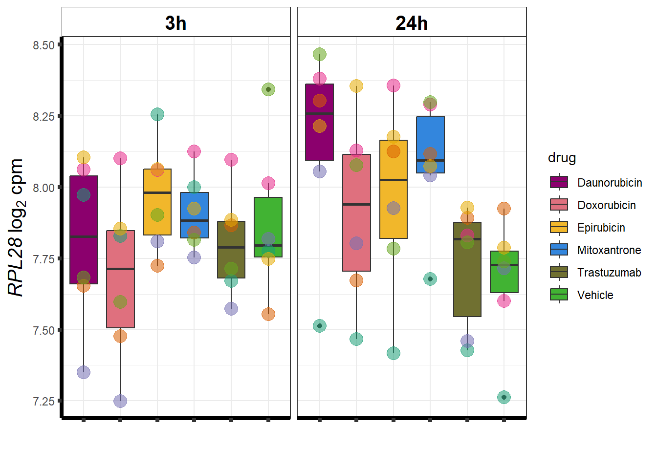
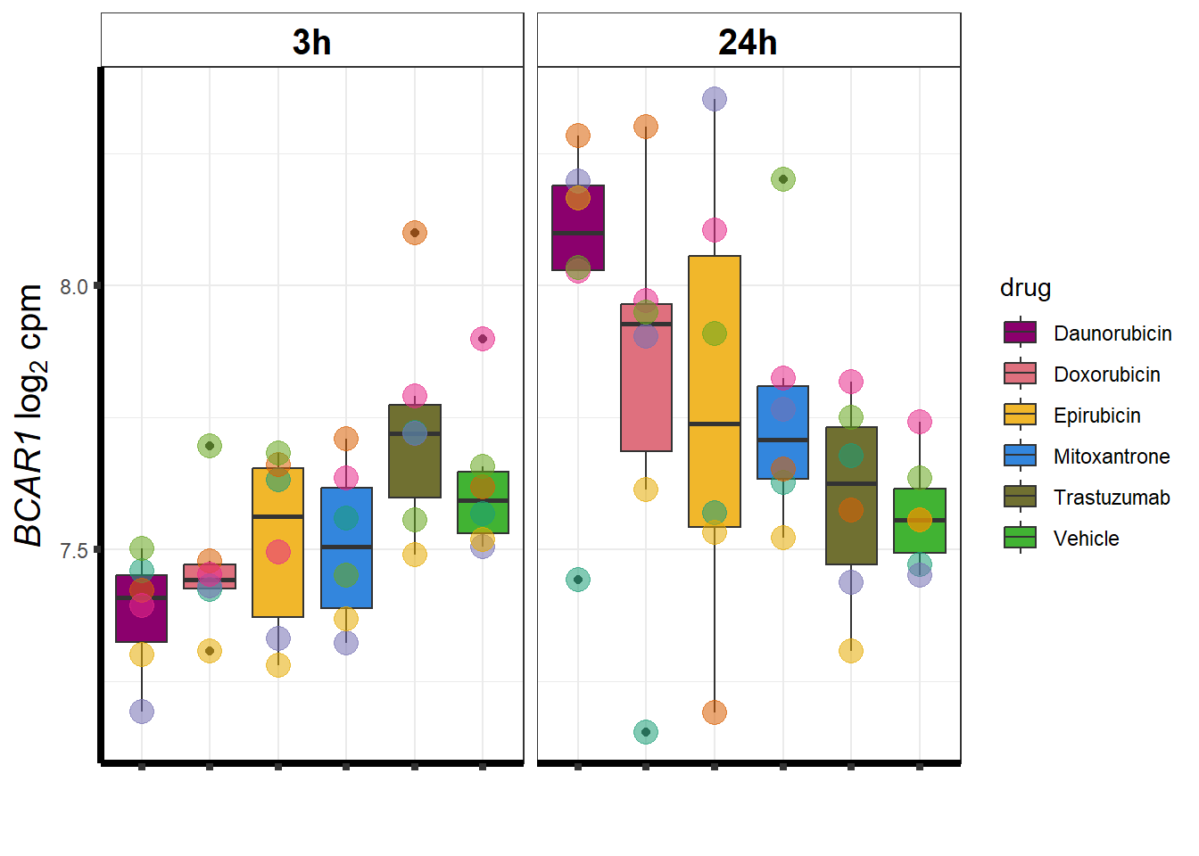
| 9564 | 9564 | BCAR1 |
| 7760 | 7760 | ZNF213 |
| 26267 | 26267 | FBXO10 |
| 5570 | 5570 | PKIB |
| 6938 | 6938 | TCF12 |
| 55132 | 55132 | LARP1B |
| 143689 | 143689 | PIWIL4 |
| 6455 | 6455 | SH3GL1 |
| 57610 | 57610 | RANBP10 |
| 337876 | 337876 | CHSY3 |
| 54520 | 54520 | CCDC93 |
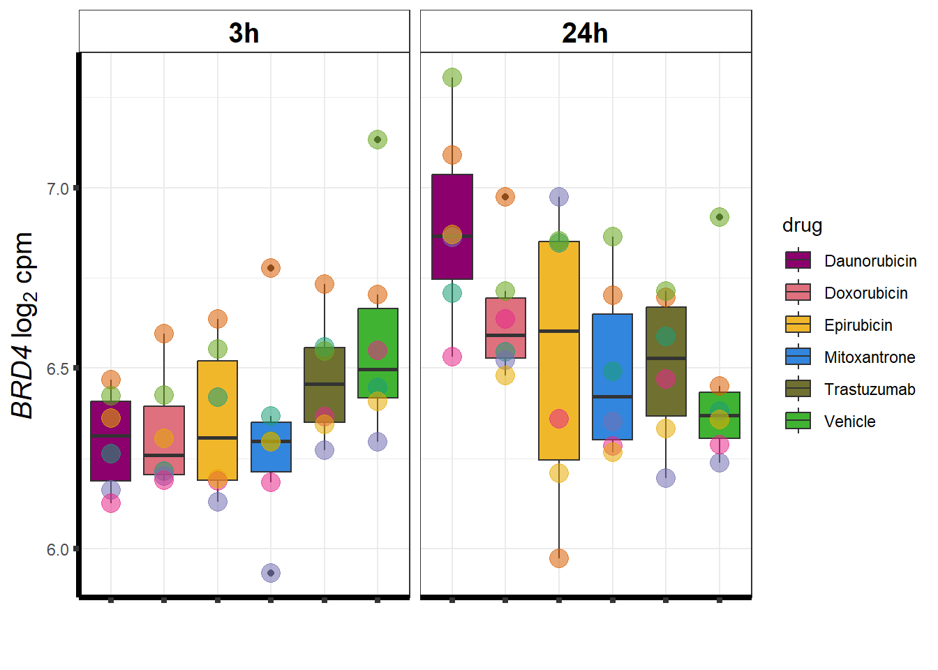
| 23476 | 23476 | BRD4 |
| 84897 | 84897 | TBRG1 |
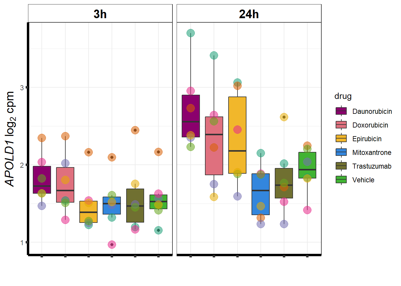
| 81575 | 81575 | APOLD1 |
| 728492 | 728492 | SERF1B |
| 285464 | 285464 | NA |
| 960 | 960 | CD44 |
| 25850 | 25850 | ZNF345 |
| 6158 | 6158 | RPL28 |
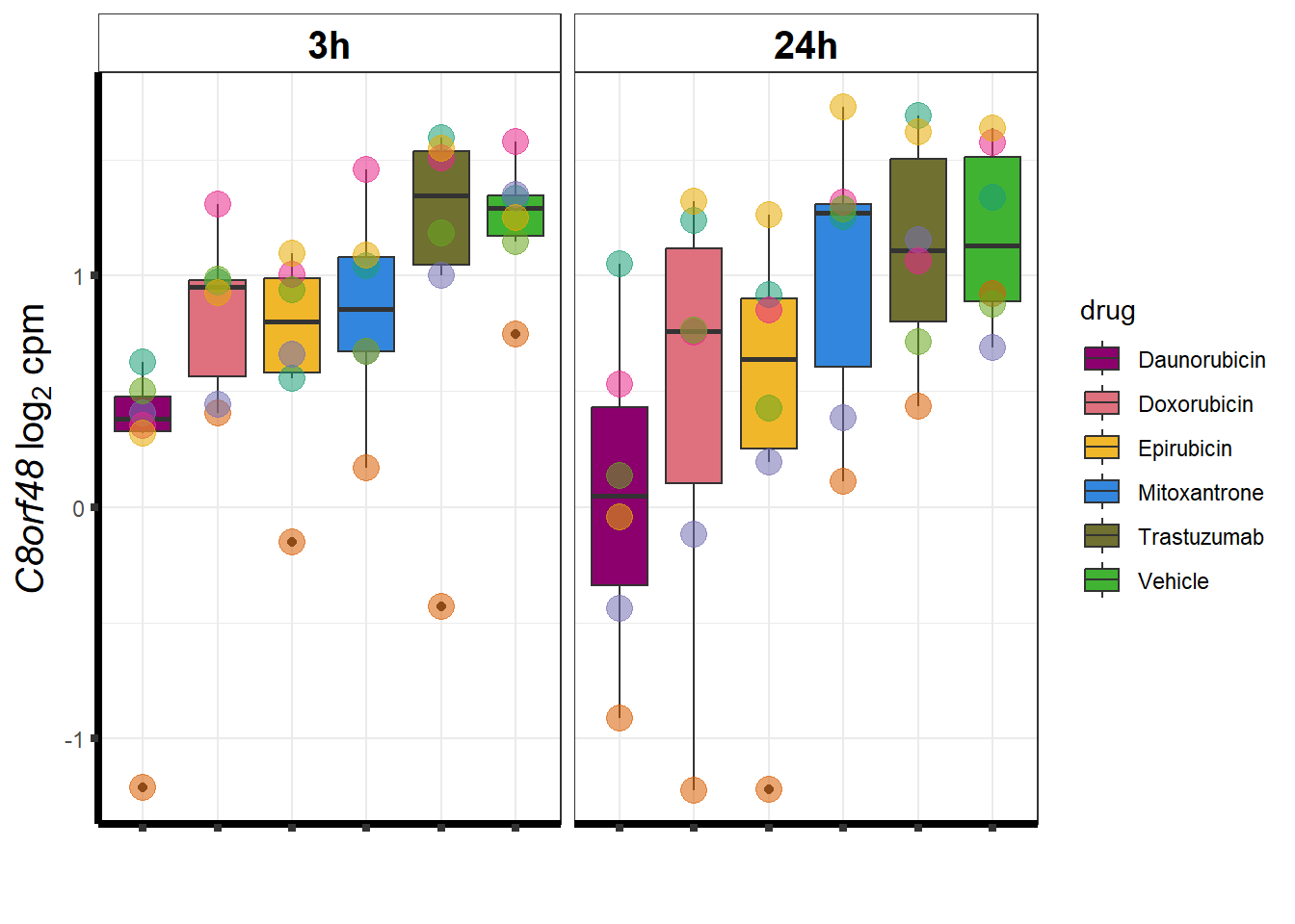
| 157773 | 157773 | C8orf48 |
| 26156 | 26156 | RSL1D1 |
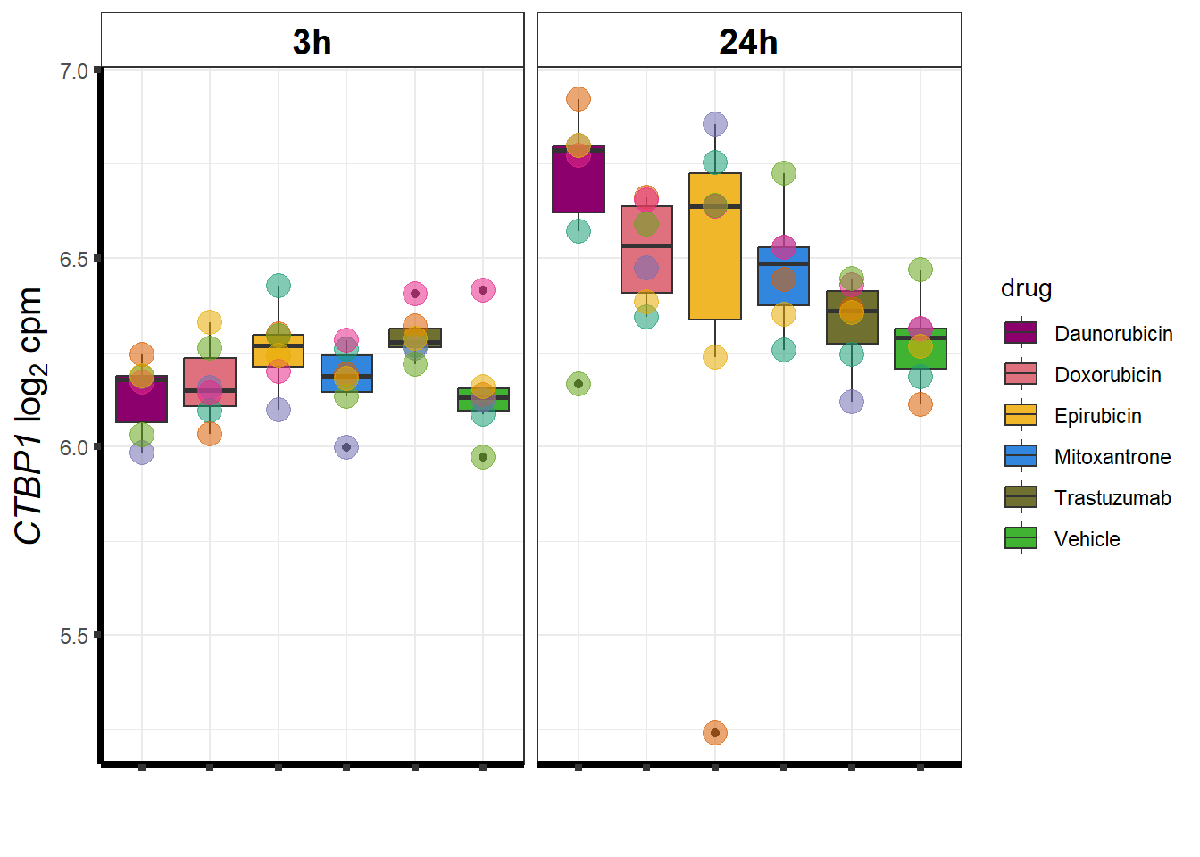
| 1487 | 1487 | CTBP1 |
| 23467 | 23467 | NPTXR |
| 91355 | 91355 | LRP5L |
| 26005 | 26005 | C2CD3 |
| 11108 | 11108 | PRDM4 |
| 25936 | 25936 | NSL1 |
| 128826 | 128826 | MIR1-1HG |
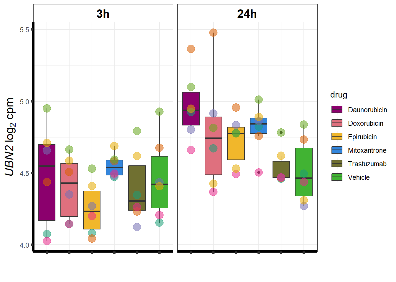
| 254048 | 254048 | UBN2 |
| 145165 | 145165 | ST13P4 |
| 105371592 | 105371592 | LOC105371592 |
| 6143 | 6143 | RPL19 |
| 57139 | 57139 | RGL3 |
| 6767 | 6767 | ST13 |
| 6992 | 6992 | PPP1R11 |
| 989 | 989 | SEPTIN7 |
| 2115 | 2115 | ETV1 |
| 643180 | 643180 | CCT6P3 |
| 4152 | 4152 | MBD1 |
| 57404 | 57404 | CYP20A1 |
| 171391 | 171391 | GATD1-DT |
| 6612 | 6612 | SUMO3 |
| 642799 | 642799 | NPIPA2 |
| 8934 | 8934 | RAB29 |
| 6722 | 6722 | SRF |
| 10628 | 10628 | TXNIP |
| 79894 | 79894 | ZNF672 |
| 118987 | 118987 | PDZD8 |
| 157697 | 157697 | ERICH1 |
| 81502 | 81502 | HM13 |
| 55787 | 55787 | TXLNG |
| 11135 | 11135 | CDC42EP1 |
| 5493 | 5493 | PPL |
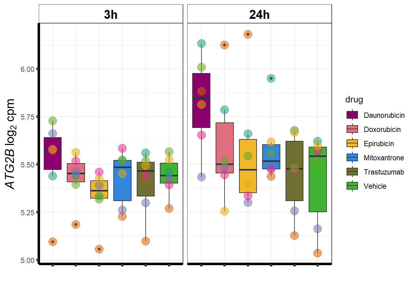
| 55102 | 55102 | ATG2B |
| 3925 | 3925 | STMN1 |
| 147700 | 147700 | KLC3 |
| 10475 | 10475 | TRIM38 |
toplist24hr %>%
  group_by(time,id) %>%
  filter(ENTREZID %in% DNRdeg_sp$ENTREZID) %>%
  filter(adj.P.Val <0.05) %>%
  # filter(id=="Daunorubicin")
  mutate(logFC=logFC*(-1)) %>%
  ggplot(., aes(x= id, y=logFC))+
  geom_boxplot(aes(fill=id))+
  theme_classic()+
  fill_palette(palette = drug_palNoVeh)+
  ggtitle("LogFC of n=131 DNR specific DEGs")+
  theme(
    plot.title = element_text(size = rel(1.5), hjust = 0.5,face = "bold"),
    axis.title = element_text(size = 15, color = "black"),
    axis.ticks = element_line(size = 1.5),
    axis.text = element_text(size = 8, color = "black", angle = 20))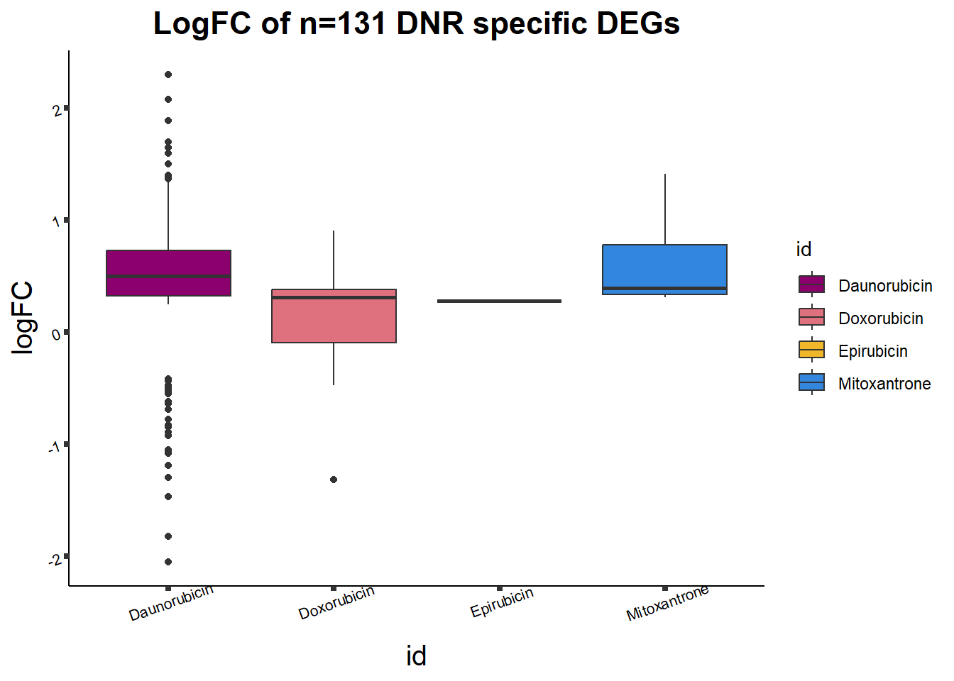
    # strip.text.x = element_text(size = 12, color = "black", face = "italic"))

toplist24hr %>%
  # filter(if_else(id=="Daunorubicin",adj.P.Val<0.01,adj.P.Val>0.01 )) %>%
  group_by(time,id) %>%
  filter(ENTREZID %in% DnronlyDEG) %>%
  filter(adj.P.Val <0.05) %>%
  ggplot(., aes(x=adj.P.Val))+
  geom_histogram(aes(fill=id))+
  geom_vline(xintercept=0.01,linetype=2)+
    # geom_density(aes(fill=id))+
    facet_wrap(~id)+
  ggtitle("DNR adj p. value <0.05")+
    fill_palette(palette = drug_palNoVeh)+
  theme_bw()+
  ggtitle("All sigDE (adj.P.val <0.05) DNR genes")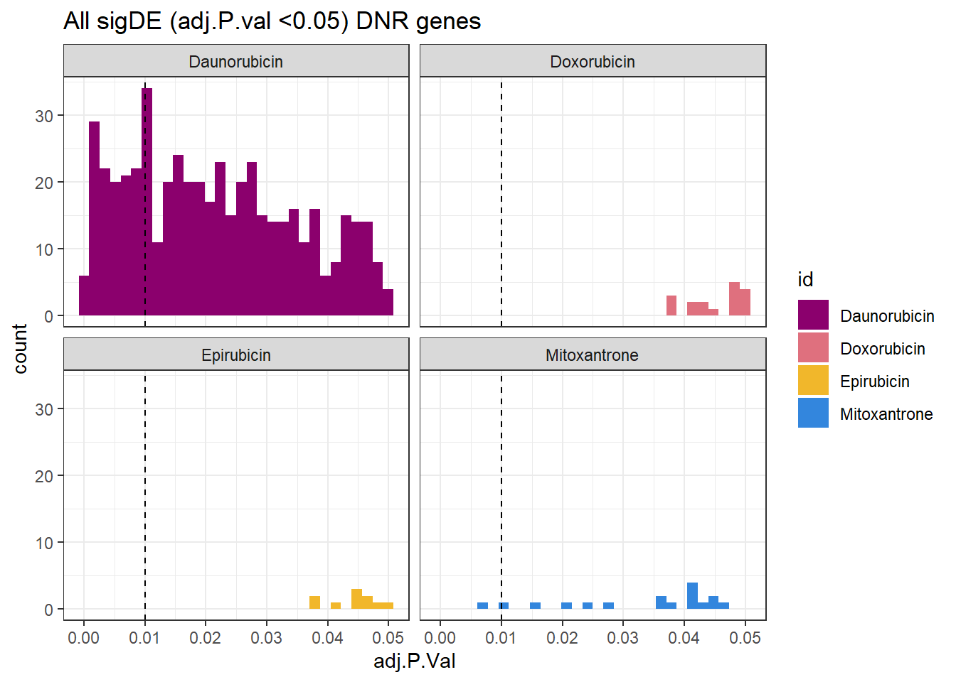
toplist24hr %>%
  filter(if_else(id=="Daunorubicin",adj.P.Val<0.01,adj.P.Val>0.01 )) %>%
  group_by(time,id) %>%
  filter(ENTREZID %in% DnronlyDEG) %>%
  filter(adj.P.Val <0.05) %>%
  ggplot(., aes(x=adj.P.Val))+
  geom_histogram(aes(fill=id))+
  geom_vline(xintercept=0.01,linetype=2)+
    # geom_density(aes(fill=id))+
    facet_wrap(~id)+
  ggtitle("DNR adj p. value <0.05")+
    fill_palette(palette = drug_palNoVeh)+
  theme_bw()+
  ggtitle("only DNR-sp genes, n=131")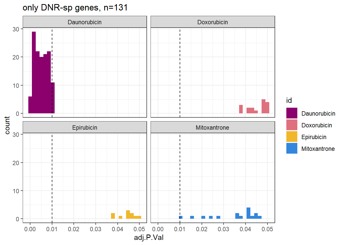
toplist24hr %>%
   filter(ENTREZID %in% DnronlyDEG) %>%

  # filter(adj.P.Val<0.05) %>%
  ggplot(., aes(x=adj.P.Val))+
  geom_density(aes(fill=id, alpha= 0.8))+
  fill_palette(palette = drug_palNoVeh)+
  theme_bw()+
  ggtitle("All sigDE (adj.P.val <0.05) DNR genes")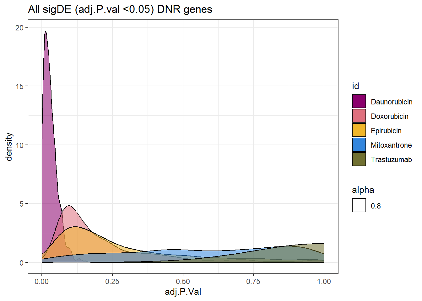
toplist24hr %>%
 filter(ENTREZID %in% DNRdeg_sp$ENTREZID) %>%
  # filter(adj.P.Val<0.05) %>%
  ggplot(., aes(x=adj.P.Val))+
  geom_density(aes(fill=id, alpha= 0.8))+
  fill_palette(palette = drug_palNoVeh)+
  theme_bw()+
  ggtitle("Only DNR specific n=131 genes")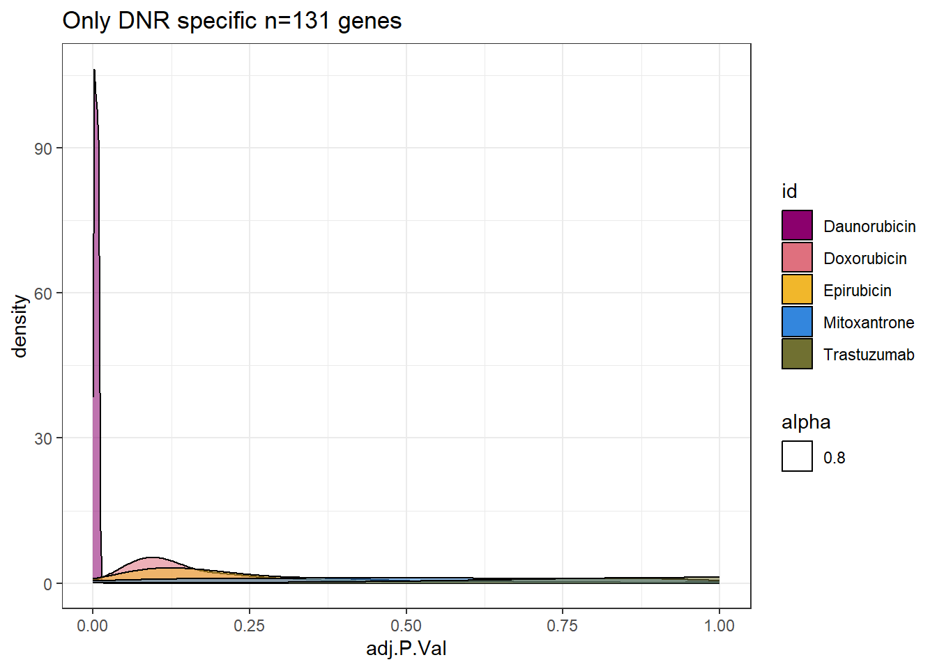
set.seed(12345)
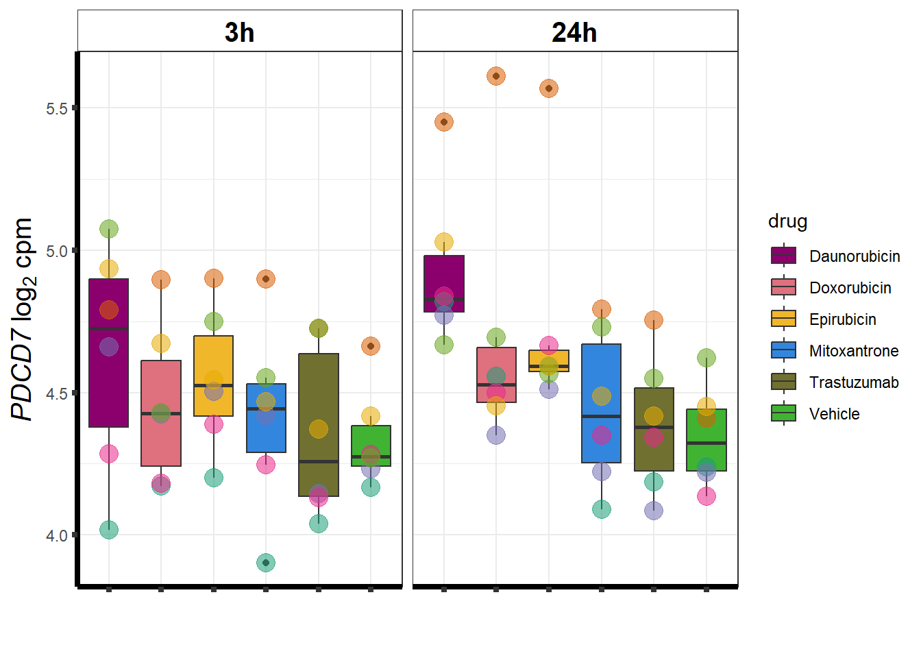
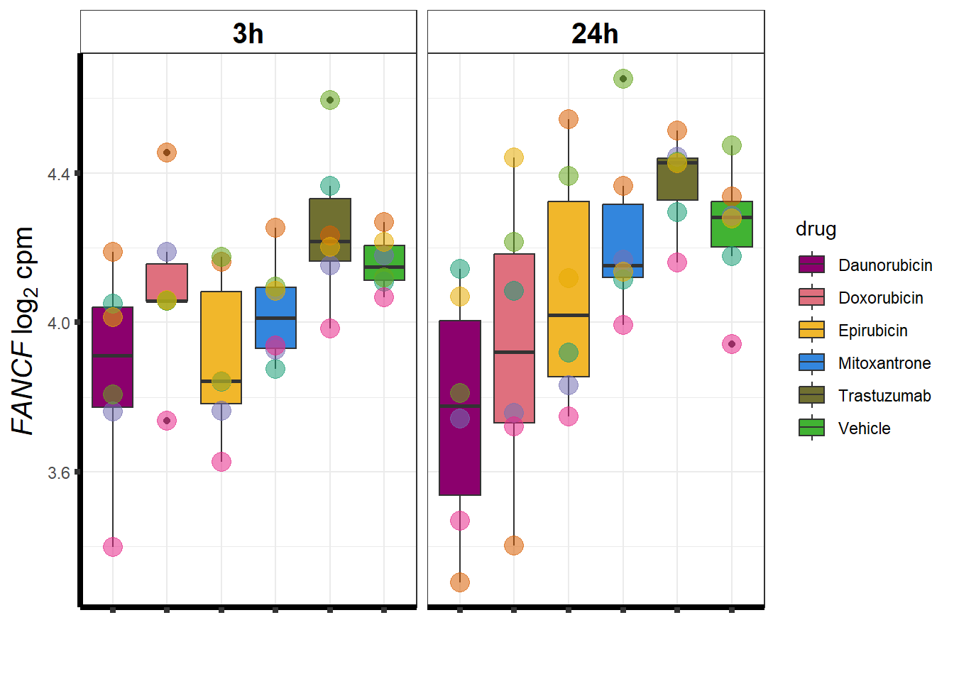
sampset <- DNRdeg_sp %>%
sample_n(.,12)
for (g in seq(from=1, to=length(sampset$ENTREZID))){
a <- sampset$SYMBOL[g]
cpm_boxplot(cpmcounts,GOI=sampset[g,1],"Dark2",drug_palc,
ylab=bquote(~italic(.(a))~log[2]~"cpm "))
}
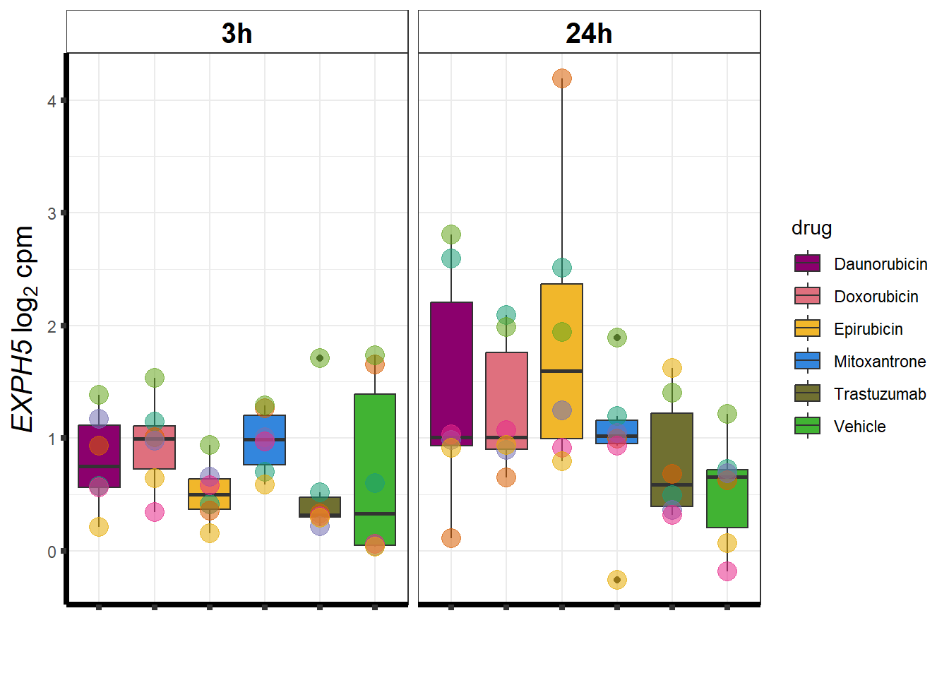
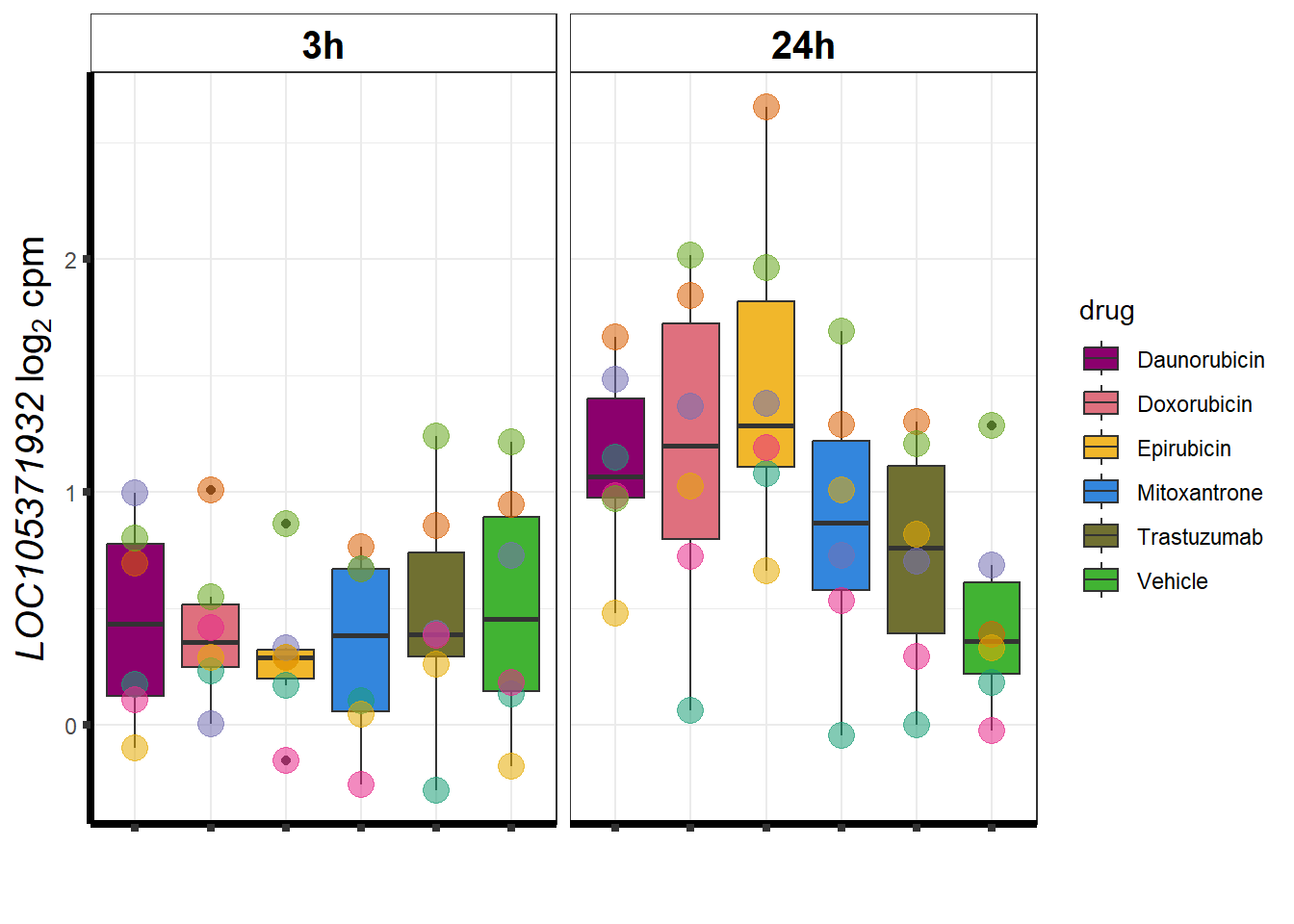
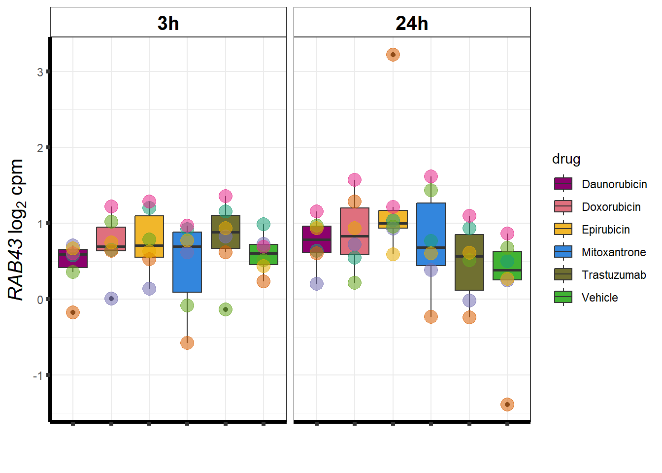
 #### Epirubicin
EPIdeg_sp <- toplist24hr %>%
  filter(if_else(id=="Epirubicin",adj.P.Val<0.01,adj.P.Val>0.01 )) %>%
  filter(ENTREZID %in% EpionlyDEG) %>%
  filter(id=="Epirubicin") %>%
  dplyr::select(ENTREZID, SYMBOL)

EPIdeg_sp %>%
  kable(., caption= "EPI specific genes") %>%
  kable_paper("striped", full_width = TRUE) %>%
  kable_styling(full_width = FALSE, font_size = 16) %>%
scroll_box( height = "500px")| ENTREZID | SYMBOL | |
|---|---|---|
| 79798 | 79798 | ARMC5 |
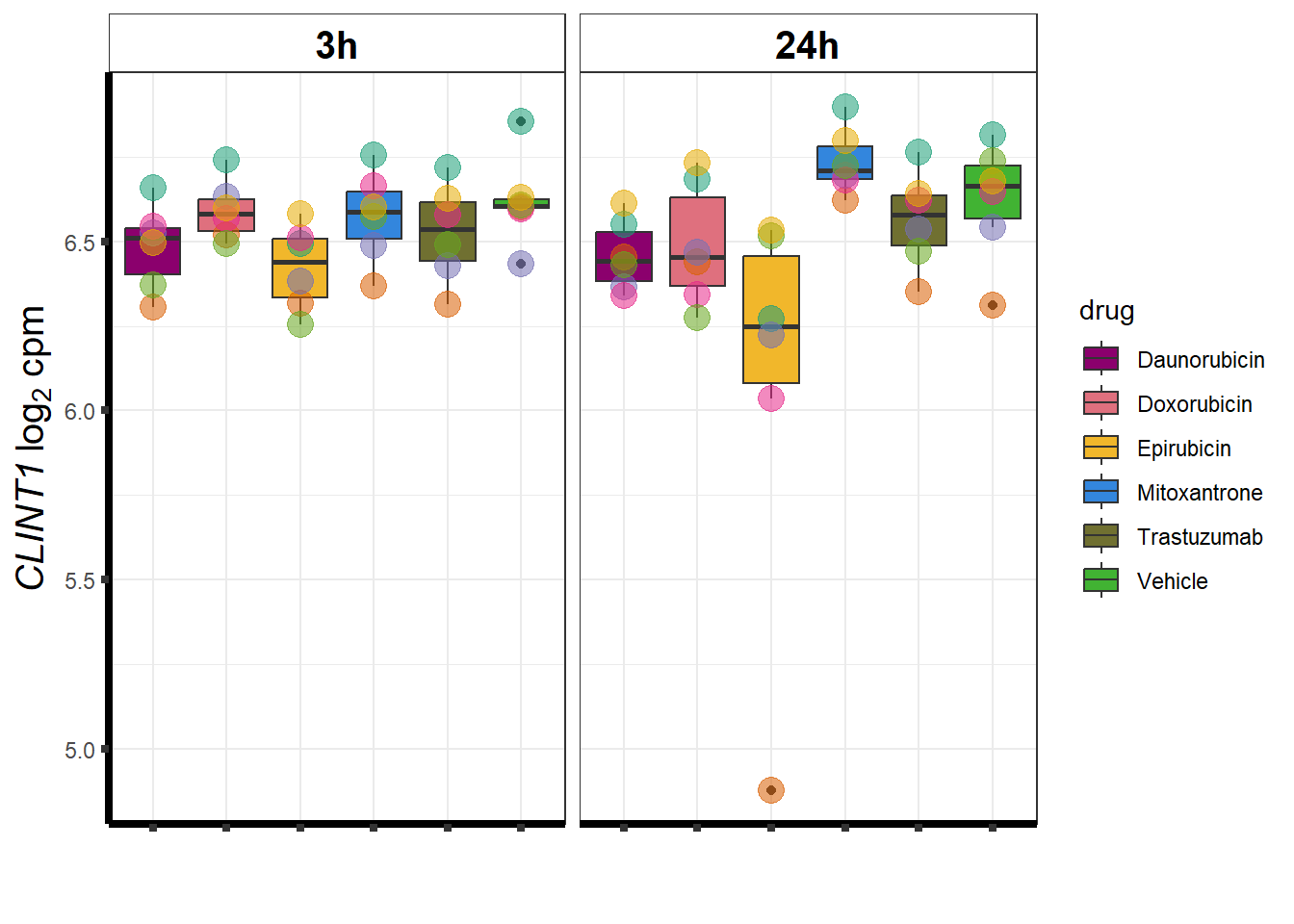
| 9685 | 9685 | CLINT1 |
| 55006 | 55006 | TRMT61B |
| 9373 | 9373 | PLAA |
| 54508 | 54508 | EPB41L4A-DT |
| 55702 | 55702 | YJU2 |
| 79759 | 79759 | ZNF668 |
| 64781 | 64781 | CERK |
| 57587 | 57587 | CFAP97 |
| 23086 | 23086 | EXPH5 |
| 90864 | 90864 | SPSB3 |
| 11097 | 11097 | NUP42 |
| 64863 | 64863 | METTL4 |
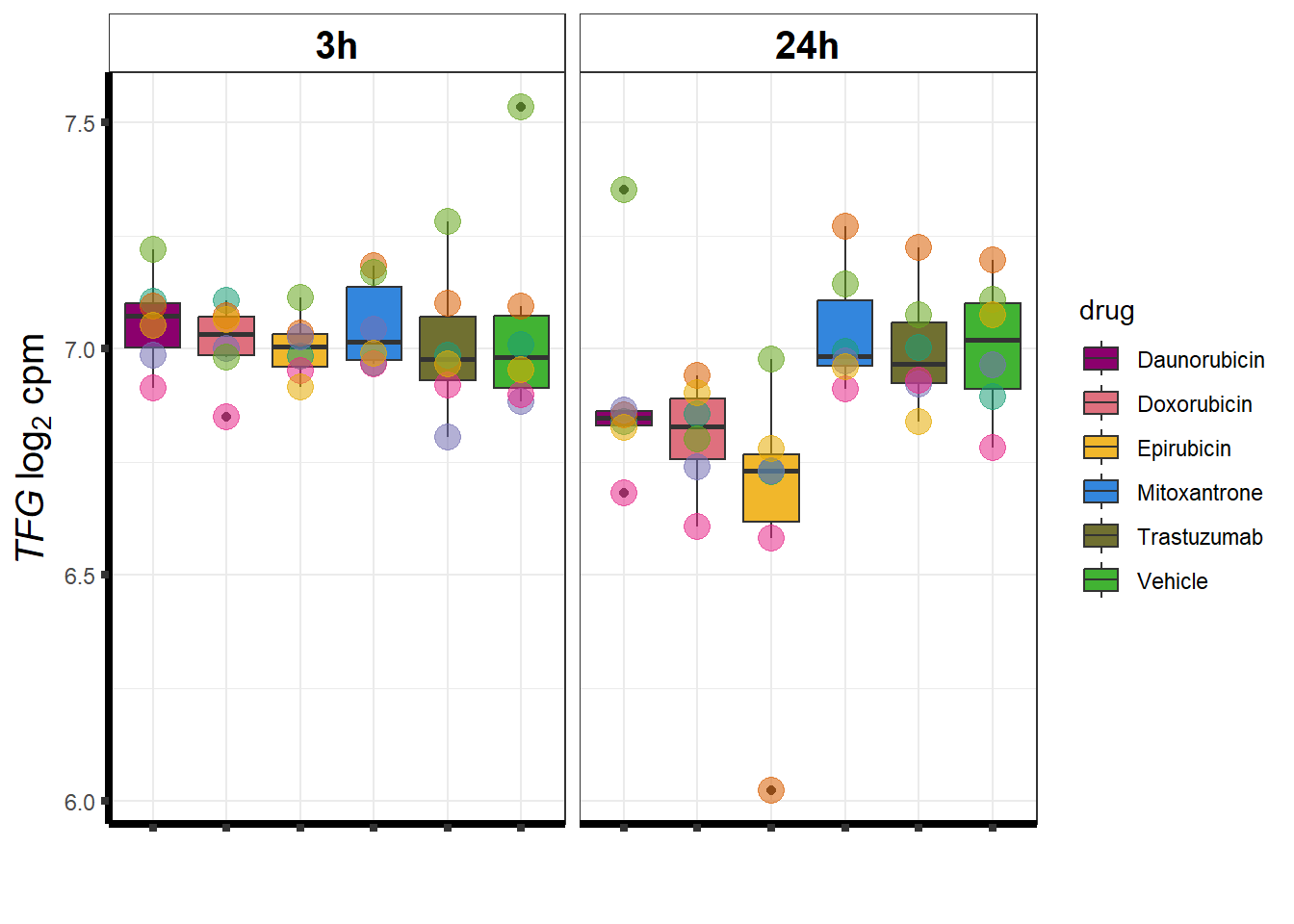
| 10342 | 10342 | TFG |
| 51132 | 51132 | RLIM |
| 57325 | 57325 | KAT14 |
| 285636 | 285636 | RIMOC1 |
| 220963 | 220963 | SLC16A9 |
| 7110 | 7110 | TMF1 |
| 51434 | 51434 | ANAPC7 |
| 55105 | 55105 | GPATCH2 |
| 92140 | 92140 | MTDH |
| 1938 | 1938 | EEF2 |
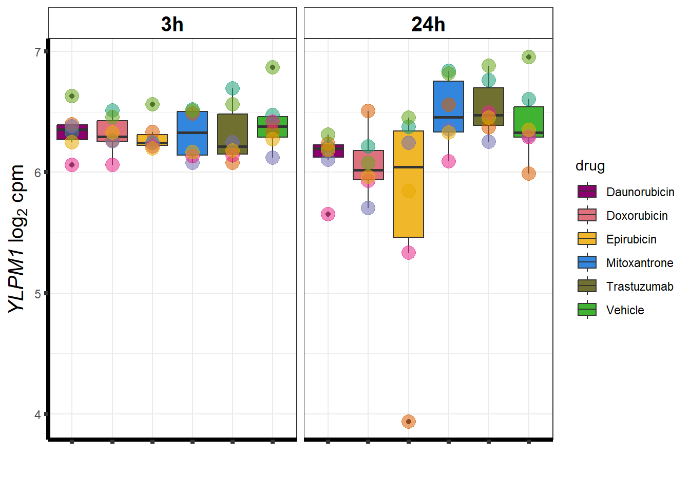
| 56252 | 56252 | YLPM1 |
| 7592 | 7592 | ZNF41 |
| 79038 | 79038 | ZFYVE21 |
| 11232 | 11232 | POLG2 |
| 339210 | 339210 | C17orf67 |
| 5884 | 5884 | RAD17 |
| 64860 | 64860 | ARMCX5 |
| 493812 | 493812 | HCG11 |
| 105371932 | 105371932 | LOC105371932 |
| 130507 | 130507 | UBR3 |
| 10111 | 10111 | RAD50 |
| 26135 | 26135 | SERBP1 |
| 27246 | 27246 | RNF115 |
| 57609 | 57609 | DIP2B |
| 85457 | 85457 | CIPC |
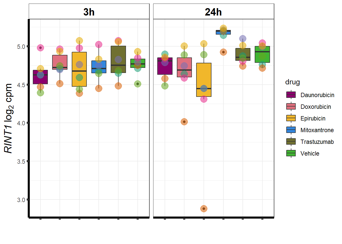
| 60561 | 60561 | RINT1 |
| 339122 | 339122 | RAB43 |
| 54942 | 54942 | ABITRAM |
| 5533 | 5533 | PPP3CC |
| 10021 | 10021 | HCN4 |
| 23122 | 23122 | CLASP2 |
| 84967 | 84967 | LSM10 |
| 340359 | 340359 | KLHL38 |
| 79713 | 79713 | IGFLR1 |
| 83852 | 83852 | SETDB2 |
| 55937 | 55937 | APOM |
| 2043 | 2043 | EPHA4 |
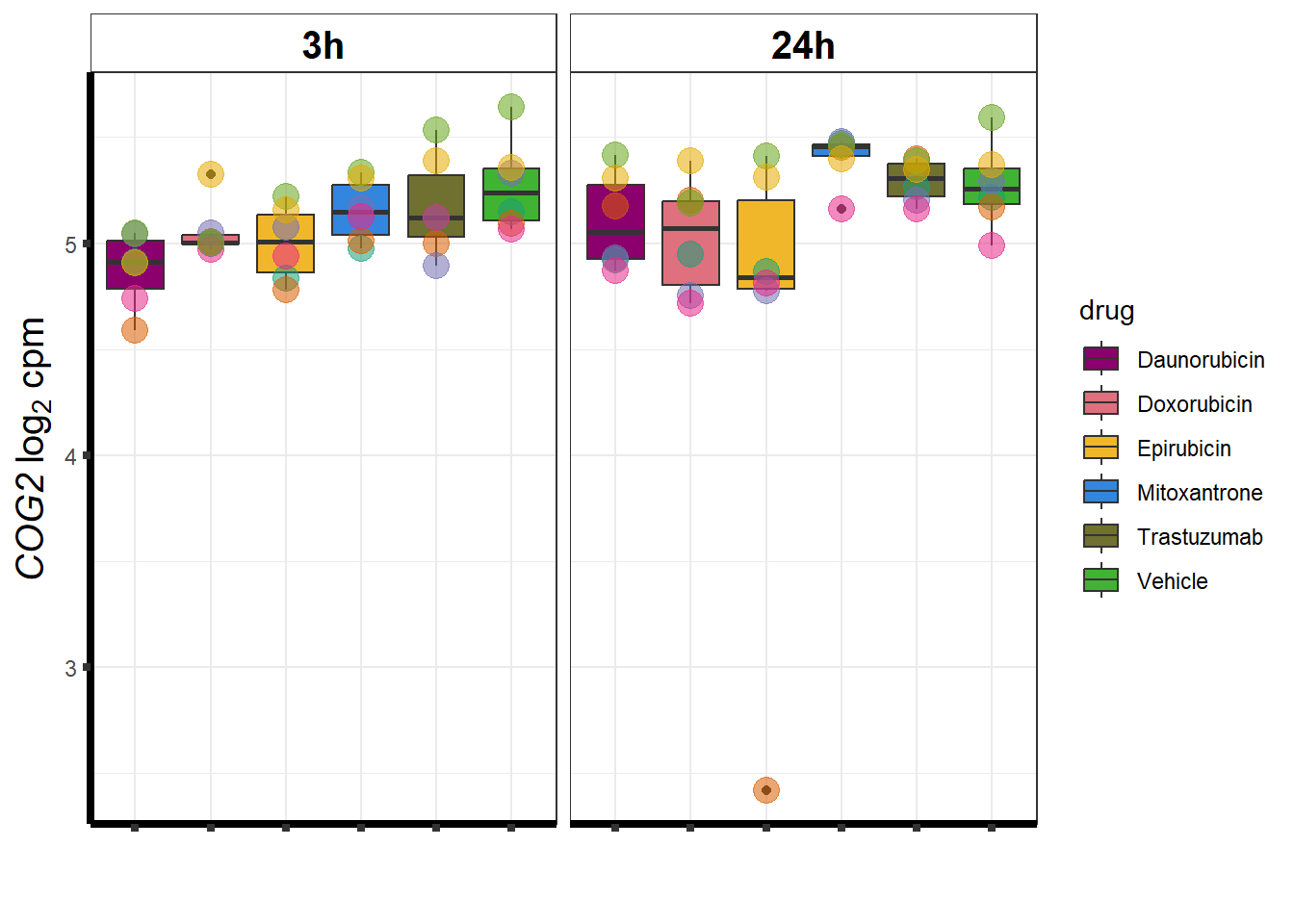
| 22796 | 22796 | COG2 |
| 1032 | 1032 | CDKN2D |
| 8624 | 8624 | PSMG1 |
| 26046 | 26046 | LTN1 |
| 64844 | 64844 | MARCHF7 |
| 1385 | 1385 | CREB1 |
| 84541 | 84541 | KBTBD8 |
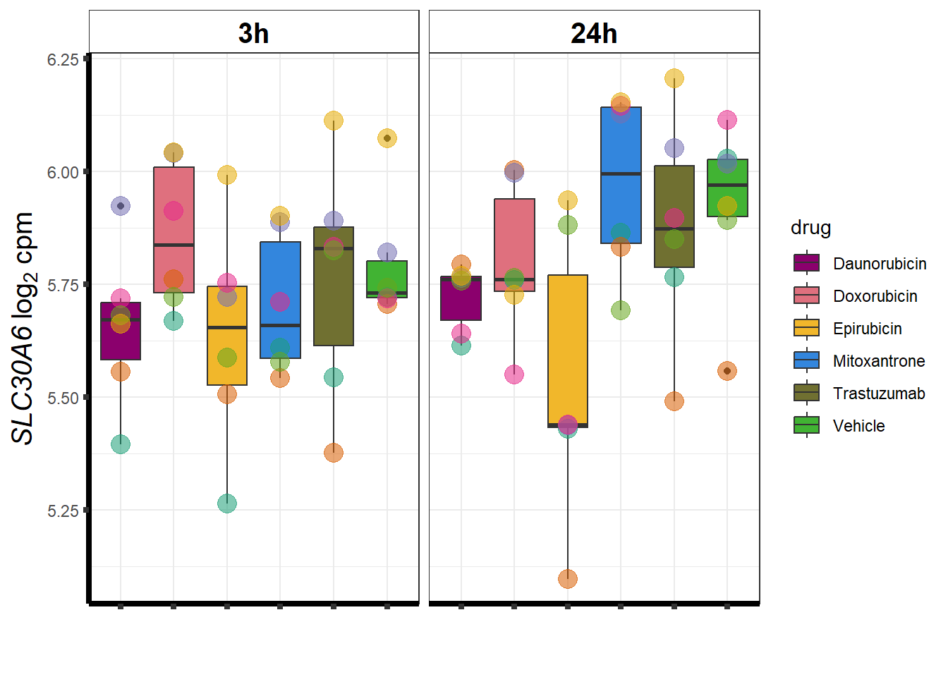
| 55676 | 55676 | SLC30A6 |
| 79797 | 79797 | ZNF408 |
| 143282 | 143282 | FGFBP3 |
| 55339 | 55339 | WDR33 |
| 79230 | 79230 | ZNF557 |
| 55223 | 55223 | TRIM62 |
| 23466 | 23466 | CBX6 |
| 201627 | 201627 | DENND6A |
| 284232 | 284232 | ANKRD20A9P |
| 7869 | 7869 | SEMA3B |
| 9972 | 9972 | NUP153 |
| 10240 | 10240 | MRPS31 |
| 63943 | 63943 | FKBPL |
| 55727 | 55727 | BTBD7 |
| 79657 | 79657 | RPAP3 |
| 23258 | 23258 | DENND5A |
| 84859 | 84859 | LRCH3 |
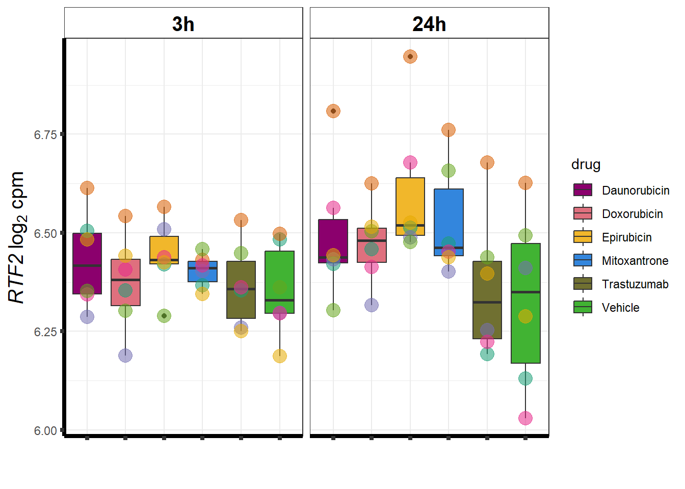
| 51507 | 51507 | RTF2 |
| 3665 | 3665 | IRF7 |
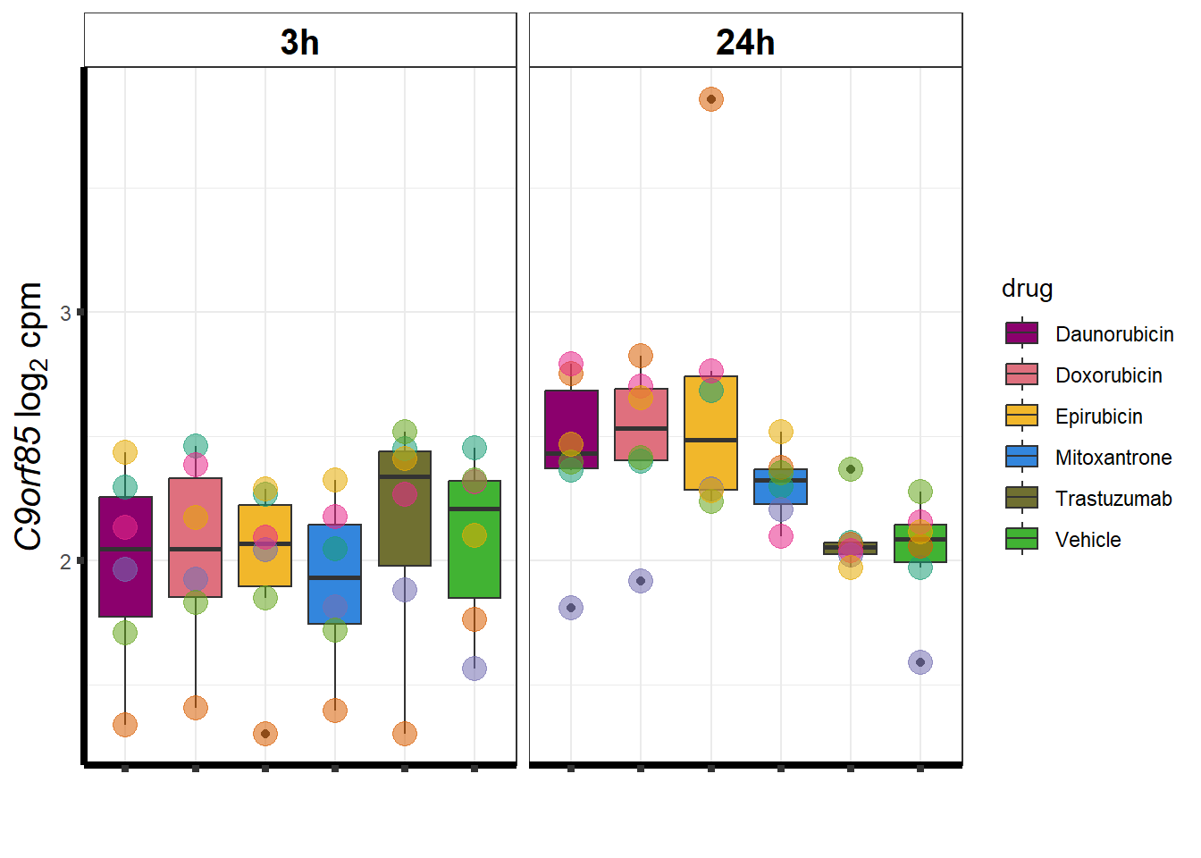
| 138241 | 138241 | C9orf85 |
| 727851 | 727851 | RGPD8 |
| 140456 | 140456 | ASB11 |
| 349136 | 349136 | WDR86 |
| 2966 | 2966 | GTF2H2 |
toplist24hr %>%
  group_by(time,id) %>%
  filter(ENTREZID %in% EPIdeg_sp$ENTREZID) %>%
  filter(adj.P.Val <0.05) %>%
  # filter(id=="Epirubicin")
  mutate(logFC=logFC*(-1)) %>%
  ggplot(., aes(x= id, y=logFC))+
  geom_boxplot(aes(fill=id))+
  theme_classic()+
  fill_palette(palette = drug_palNoVeh)+
  ggtitle("LogFC of n=81 EPI specific DEGs")+
  theme(
    plot.title = element_text(size = rel(1.5), hjust = 0.5,face = "bold"),
    axis.title = element_text(size = 15, color = "black"),
    axis.ticks = element_line(size = 1.5),
    axis.text = element_text(size = 8, color = "black", angle = 20))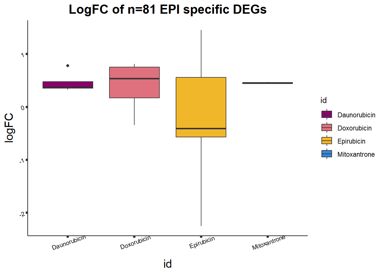
    # strip.text.x = element_text(size = 12, color = "black", face = "italic"))

toplist24hr %>%
  filter(if_else(id=="Epirubicin",adj.P.Val<0.01,adj.P.Val>0.01 )) %>%
  group_by(time,id) %>%
  filter(ENTREZID %in% EpionlyDEG) %>%
  filter(adj.P.Val <0.05) %>%
  ggplot(., aes(x=adj.P.Val))+
  geom_histogram(aes(fill=id))+
  geom_vline(xintercept=0.01,linetype=2)+
    # geom_density(aes(fill=id))+
    facet_wrap(~id)+
  ggtitle("EPI adj p. value <0.05")+
    fill_palette(palette = drug_palNoVeh)+
  theme_bw() +
  ggtitle("only showing EPI n=81 specific genes ")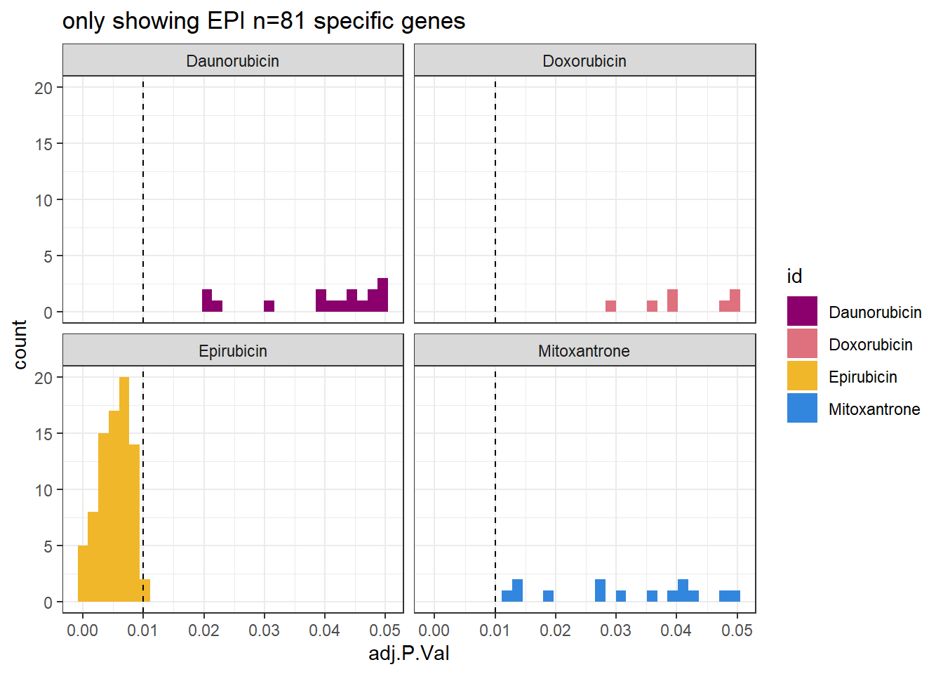
toplist24hr %>%
  filter(ENTREZID %in% EpionlyDEG) %>%
  # filter(adj.P.Val<0.05) %>%
  ggplot(., aes(x=adj.P.Val))+
  geom_density(aes(fill=id, alpha= 0.8))+
  fill_palette(palette = drug_palNoVeh)+
  theme_bw()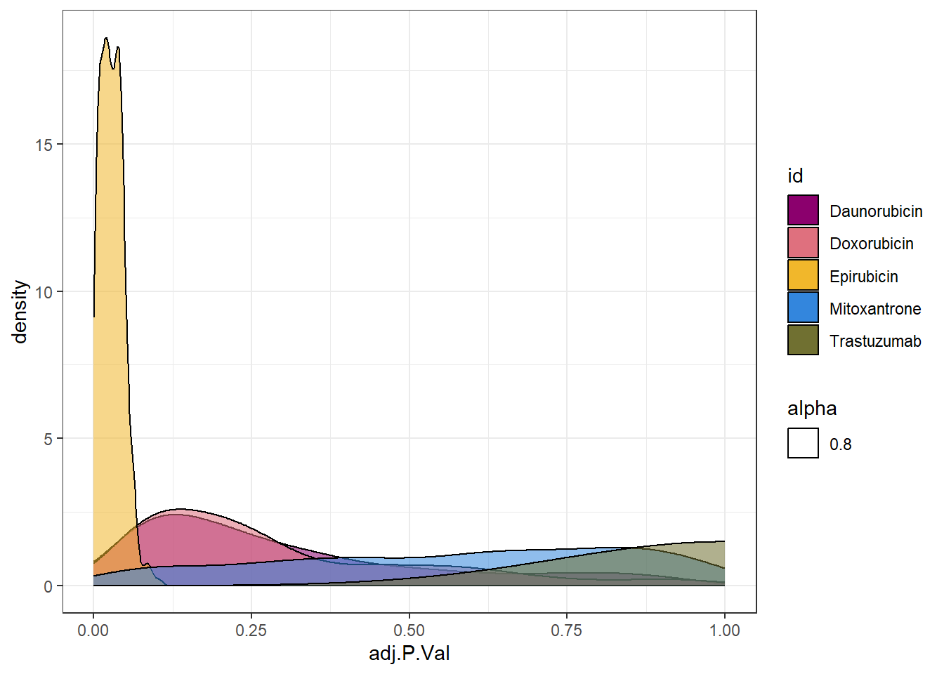
set.seed(12345)
sampset <- EPIdeg_sp %>%
  sample_n(.,12)

for (g in seq(from=1, to=length(sampset$ENTREZID))){
  a <- sampset$SYMBOL[g]
  cpm_boxplot(cpmcounts,GOI=sampset[g,1],"Dark2",drug_palc,
                ylab=bquote(~italic(.(a))~log[2]~"cpm "))
}
sessionInfo()R version 4.2.2 (2022-10-31 ucrt)
Platform: x86_64-w64-mingw32/x64 (64-bit)
Running under: Windows 10 x64 (build 19045)
Matrix products: default
locale:
[1] LC_COLLATE=English_United States.utf8
[2] LC_CTYPE=English_United States.utf8
[3] LC_MONETARY=English_United States.utf8
[4] LC_NUMERIC=C
[5] LC_TIME=English_United States.utf8
attached base packages:
[1] grid stats graphics grDevices utils datasets methods
[8] base
other attached packages:
[1] ComplexHeatmap_2.12.1 broom_1.0.5 kableExtra_1.3.4
[4] sjmisc_2.8.9 scales_1.2.1 ggpubr_0.6.0
[7] cowplot_1.1.1 RColorBrewer_1.1-3 biomaRt_2.52.0
[10] ggsignif_0.6.4 lubridate_1.9.2 forcats_1.0.0
[13] stringr_1.5.0 dplyr_1.1.2 purrr_1.0.1
[16] readr_2.1.4 tidyr_1.3.0 tibble_3.2.1
[19] ggplot2_3.4.2 tidyverse_2.0.0 limma_3.52.4
[22] workflowr_1.7.0
loaded via a namespace (and not attached):
[1] backports_1.4.1 circlize_0.4.15 BiocFileCache_2.4.0
[4] systemfonts_1.0.4 GenomeInfoDb_1.32.4 digest_0.6.31
[7] foreach_1.5.2 htmltools_0.5.5 fansi_1.0.4
[10] magrittr_2.0.3 memoise_2.0.1 cluster_2.1.4
[13] doParallel_1.0.17 tzdb_0.4.0 Biostrings_2.64.1
[16] matrixStats_1.0.0 svglite_2.1.1 timechange_0.2.0
[19] prettyunits_1.1.1 RVenn_1.1.0 colorspace_2.1-0
[22] blob_1.2.4 rvest_1.0.3 rappdirs_0.3.3
[25] xfun_0.39 callr_3.7.3 crayon_1.5.2
[28] RCurl_1.98-1.12 jsonlite_1.8.5 iterators_1.0.14
[31] glue_1.6.2 gtable_0.3.3 zlibbioc_1.42.0
[34] XVector_0.36.0 webshot_0.5.4 GetoptLong_1.0.5
[37] car_3.1-2 shape_1.4.6 BiocGenerics_0.42.0
[40] abind_1.4-5 futile.options_1.0.1 DBI_1.1.3
[43] rstatix_0.7.2 Rcpp_1.0.10 viridisLite_0.4.2
[46] progress_1.2.2 units_0.8-2 clue_0.3-64
[49] proxy_0.4-27 bit_4.0.5 stats4_4.2.2
[52] httr_1.4.6 pkgconfig_2.0.3 XML_3.99-0.14
[55] farver_2.1.1 sass_0.4.6 dbplyr_2.3.2
[58] utf8_1.2.3 tidyselect_1.2.0 labeling_0.4.2
[61] rlang_1.1.1 later_1.3.1 AnnotationDbi_1.58.0
[64] munsell_0.5.0 tools_4.2.2 cachem_1.0.8
[67] cli_3.6.1 generics_0.1.3 RSQLite_2.3.1
[70] ggVennDiagram_1.2.2 sjlabelled_1.2.0 evaluate_0.21
[73] fastmap_1.1.1 yaml_2.3.7 processx_3.8.1
[76] knitr_1.43 bit64_4.0.5 fs_1.6.2
[79] KEGGREST_1.36.3 whisker_0.4.1 formatR_1.14
[82] xml2_1.3.4 compiler_4.2.2 rstudioapi_0.14
[85] filelock_1.0.2 curl_5.0.1 png_0.1-8
[88] e1071_1.7-13 bslib_0.5.0 stringi_1.7.12
[91] highr_0.10 ps_1.7.5 futile.logger_1.4.3
[94] classInt_0.4-9 vctrs_0.6.3 pillar_1.9.0
[97] lifecycle_1.0.3 jquerylib_0.1.4 GlobalOptions_0.1.2
[100] bitops_1.0-7 insight_0.19.2 httpuv_1.6.11
[103] R6_2.5.1 promises_1.2.0.1 KernSmooth_2.23-21
[106] IRanges_2.30.1 codetools_0.2-19 lambda.r_1.2.4
[109] rprojroot_2.0.3 rjson_0.2.21 withr_2.5.0
[112] S4Vectors_0.34.0 GenomeInfoDbData_1.2.8 parallel_4.2.2
[115] hms_1.1.3 VennDiagram_1.7.3 class_7.3-22
[118] rmarkdown_2.22 carData_3.0-5 git2r_0.32.0
[121] sf_1.0-13 getPass_0.2-2 Biobase_2.56.0