Run1_analysis
ERM
20230118
Last updated: 2023-02-10
Checks: 7 0
Knit directory: Cardiotoxicity/
This reproducible R Markdown analysis was created with workflowr (version 1.7.0). The Checks tab describes the reproducibility checks that were applied when the results were created. The Past versions tab lists the development history.
Great! Since the R Markdown file has been committed to the Git repository, you know the exact version of the code that produced these results.
Great job! The global environment was empty. Objects defined in the global environment can affect the analysis in your R Markdown file in unknown ways. For reproduciblity it’s best to always run the code in an empty environment.
The command set.seed(20230109) was run prior to running
the code in the R Markdown file. Setting a seed ensures that any results
that rely on randomness, e.g. subsampling or permutations, are
reproducible.
Great job! Recording the operating system, R version, and package versions is critical for reproducibility.
Nice! There were no cached chunks for this analysis, so you can be confident that you successfully produced the results during this run.
Great job! Using relative paths to the files within your workflowr project makes it easier to run your code on other machines.
Great! You are using Git for version control. Tracking code development and connecting the code version to the results is critical for reproducibility.
The results in this page were generated with repository version 7a6d5d5. See the Past versions tab to see a history of the changes made to the R Markdown and HTML files.
Note that you need to be careful to ensure that all relevant files for
the analysis have been committed to Git prior to generating the results
(you can use wflow_publish or
wflow_git_commit). workflowr only checks the R Markdown
file, but you know if there are other scripts or data files that it
depends on. Below is the status of the Git repository when the results
were generated:
Ignored files:
    Ignored:    .RData
    Ignored:    .Rhistory
    Ignored:    .Rproj.user/
    Ignored:    data/.txt
    Ignored:    data/allgenes.txt
    Ignored:    data/backGL.txt
    Ignored:    data/data_outline.txt
    Ignored:    data/filenameonly.txt
    Ignored:    data/individualDRCfile.RDS
    Ignored:    data/mymatrix.RDS
    Ignored:    data/norm_LDH.csv
    Ignored:    data/norm_counts.csv
    Ignored:    data/response_cluster24h.csv
    Ignored:    data/sigVDA24.txt
    Ignored:    data/sigVDA3.txt
    Ignored:    data/sigVDX24.txt
    Ignored:    data/sigVDX3.txt
    Ignored:    data/sigVEP24.txt
    Ignored:    data/sigVEP3.txt
    Ignored:    data/sigVMT24.txt
    Ignored:    data/sigVMT3.txt
    Ignored:    data/sigVTR24.txt
    Ignored:    data/sigVTR3.txt

Untracked files:
    Untracked:  .RDataTmp
    Untracked:  firstvenn24h.png
    Untracked:  mcor.csv
    Untracked:  reneebasecode.R

Unstaged changes:
    Modified:   code/Corrscripts.R
    Modified:   venn_code.R
Note that any generated files, e.g. HTML, png, CSS, etc., are not included in this status report because it is ok for generated content to have uncommitted changes.
These are the previous versions of the repository in which changes were
made to the R Markdown (analysis/RNAseqanalysis.Rmd) and
HTML (docs/RNAseqanalysis.html) files. If you’ve configured
a remote Git repository (see ?wflow_git_remote), click on
the hyperlinks in the table below to view the files as they were in that
past version.
| File | Version | Author | Date | Message |
|---|---|---|---|---|
| Rmd | 7a6d5d5 | reneeisnowhere | 2023-02-10 | updates for the week part 500 |
| html | cdd9374 | reneeisnowhere | 2023-02-10 | Build site. |
| Rmd | 40fb340 | reneeisnowhere | 2023-02-10 | updates for the week |
| Rmd | accc241 | reneeisnowhere | 2023-02-10 | updates for the week |
| Rmd | 1fc5c19 | reneeisnowhere | 2023-02-09 | Git update |
Hello! I am first loading all the beautiful libraries I will need.
library(Biobase)
library(edgeR)
library(limma)
library(RColorBrewer)
library(mixOmics)
library(VennDiagram)
library(HTSFilter)
library(ggplot2)
library(gridExtra)
library(reshape2)
library(devtools)
library(AnnotationHub)
library(tidyverse)
library(scales)
library(biomaRt)
library(Homo.sapiens)
library(cowplot)
library(ggrepel)
library(corrplot)
library(Hmisc)
The next step is to load all the data I will be using. Currently, I am not posting the raw data, but I will release in the future.
This is how I retrieved the gene symbols.
 ###now we add genenames to the geneid###

geneid <- rownames(mymatrix) ### pulls the names we have in the counts file
genes <- select(Homo.sapiens, keys=geneid, columns=c("SYMBOL"),
  keytype="ENTREZID")
genes <- genes[!duplicated(genes$ENTREZID),]
mymatrix$genes <- genes
Filtering out low count genes
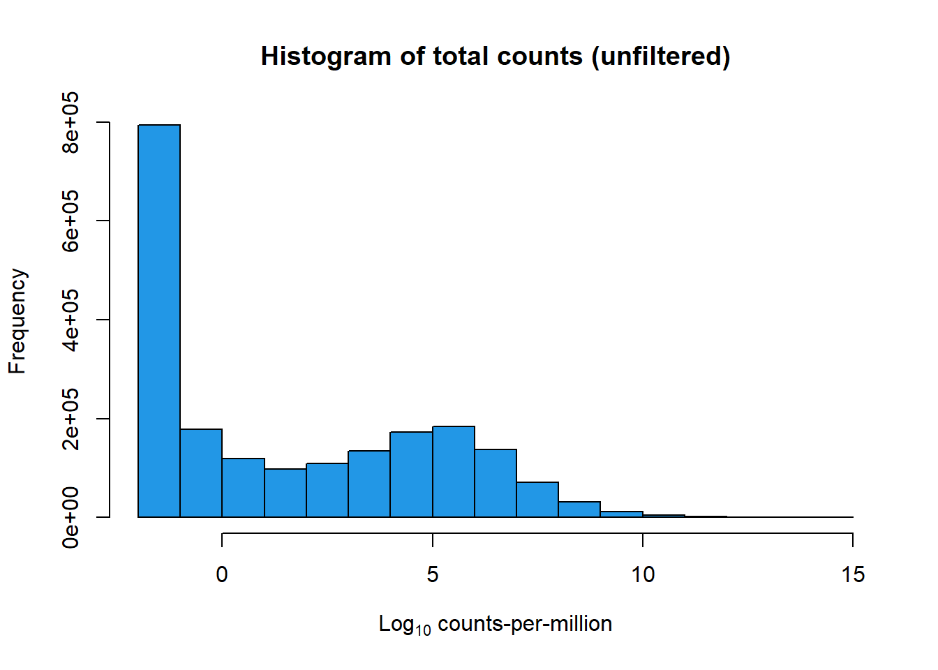
Filtering the genes that are lowly expressed using several methods.
First method, removing only those rows with zero counts across all samples.
#
# old.par <- par(mar = c(0, 0, 0, 0))
# par(old.par)
# boxplot(data =RNAseqreads, total~Sample, main = "Boxplots of total reads",xaxt = "n", xlab= "")
# x_axis_labels(labels = samplenames, every_nth = 1, adj=1, srt =90, cex =0.4)
# ggplot(RNAseqreads, x = Sample, y = total)+
#   geom_boxplot()

table(rowSums(mymatrix$counts==0)==72)
FALSE  TRUE
24931  3464
This filtering would leave 24931 genes and remove 3464, That is too many leftover genes!
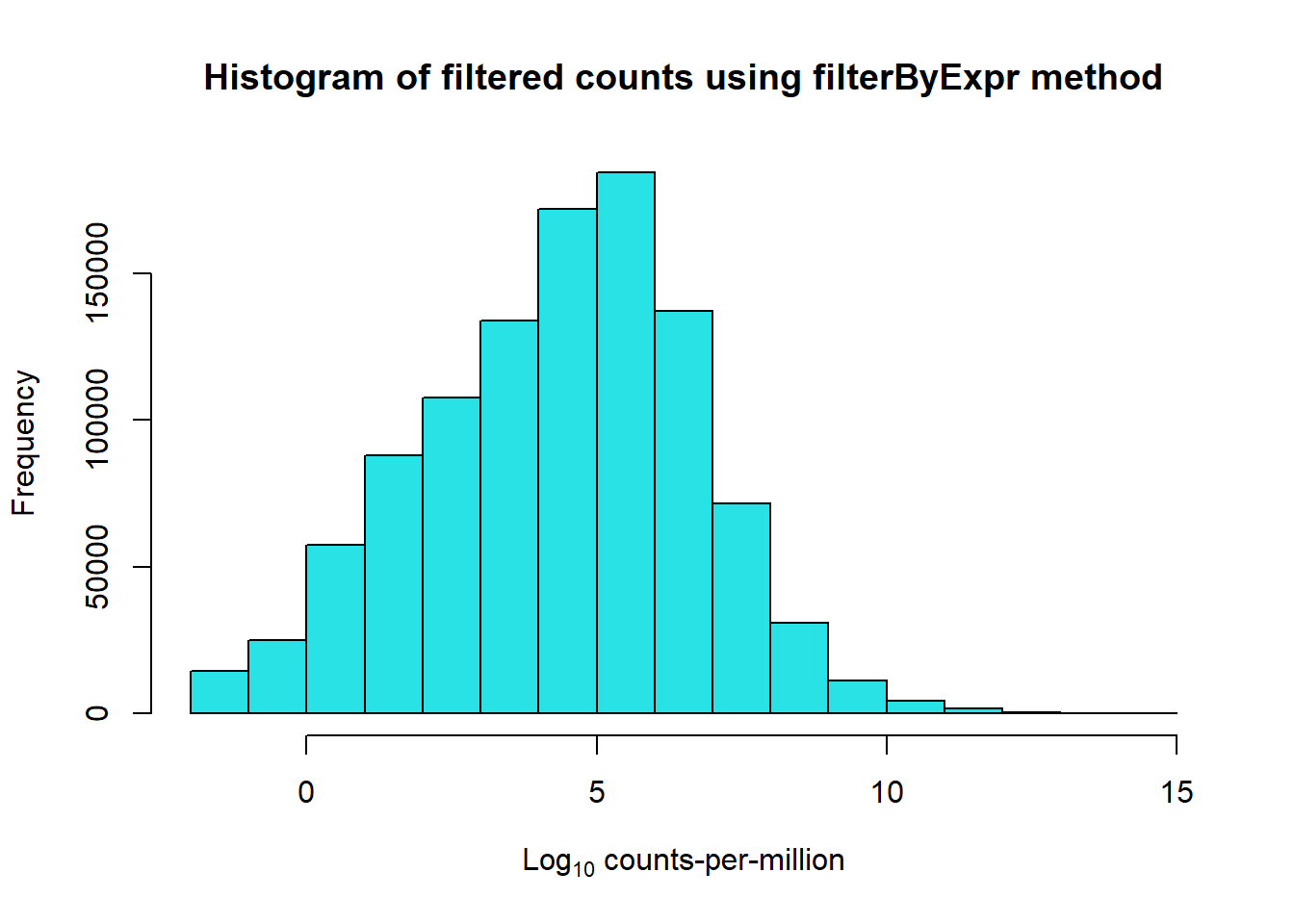
So now to try something a little more stringent using the built in function from the edgeR package.
keep <- filterByExpr.DGEList(mymatrix, group = group)
filter_test <- mymatrix[keep, , keep.lib.sizes=FALSE]
dim(filter_test)
[1] 14448 72This method effectively uses a cutoff off that leaves 14448 genes.
The cutoff is determined by keeping genes that have a count-per-million
(CPM) above 10, (the default minimum set) in 6 samples. A set is
determined using the design matrix.
For my design, I grouped my 72 samples into sets of 6, one set includes
each individual + a specific treatment + a specific time.
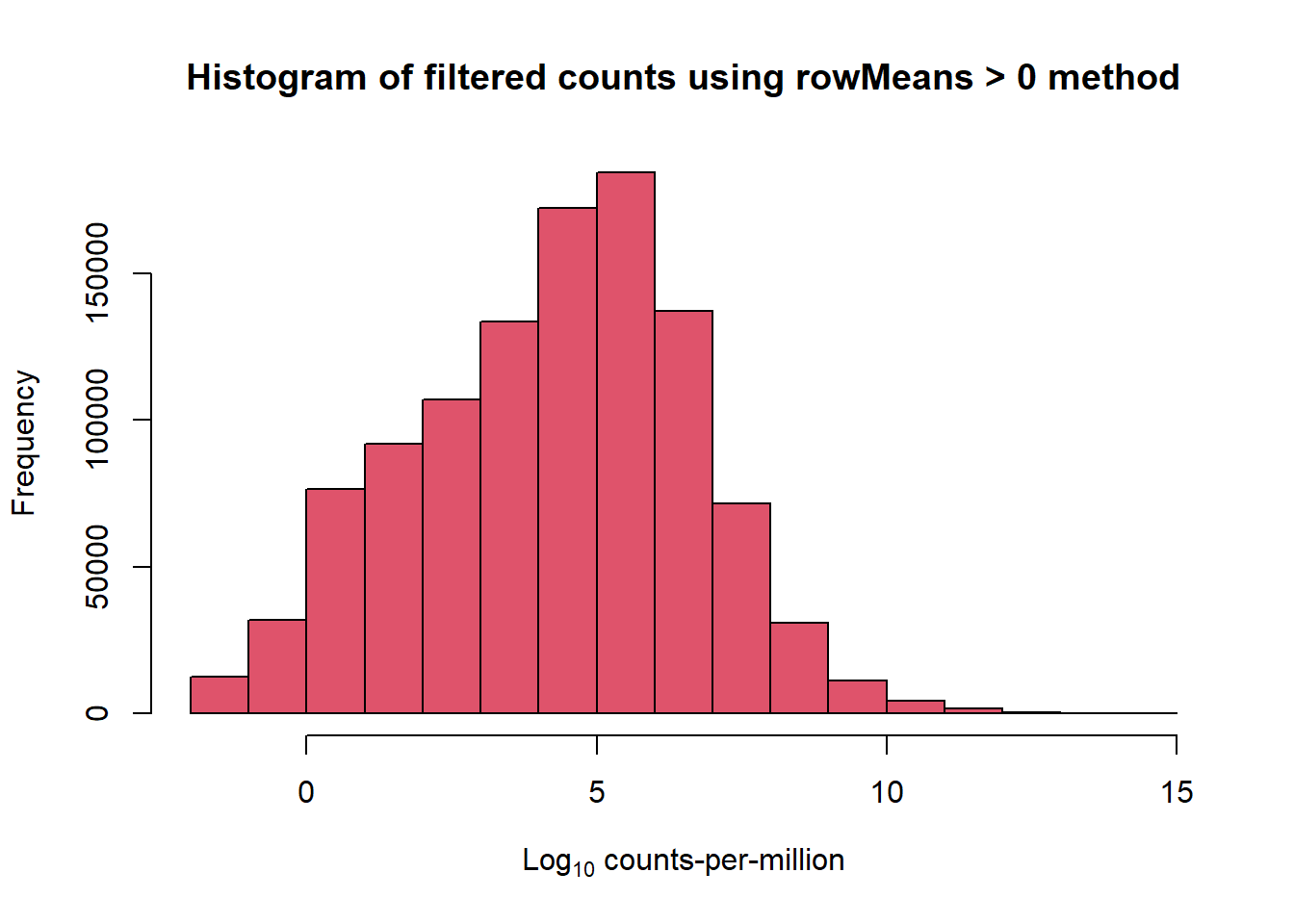
The beginning cutoff-standard in our lab is to start by using the rowMeans >0 cutoff on the log10 of cpm.
cpm <- cpm(mymatrix)
lcpm <- cpm(mymatrix, log=TRUE)  ### for determining the basic cutoffs
dim(lcpm)
[1] 28395 72L <- mean(mymatrix$samples$lib.size) * 1e-6
M <- median(mymatrix$samples$lib.size) * 1e-6
c(L, M)[1] 4.679061 4.494188filcpm_matrix <- subset(lcpm, (rowMeans(lcpm)>0))
dim(filcpm_matrix)[1] 14823 72##method 2 with rowMeans
row_means <- rowMeans(lcpm)
x <- mymatrix[row_means > 0,]
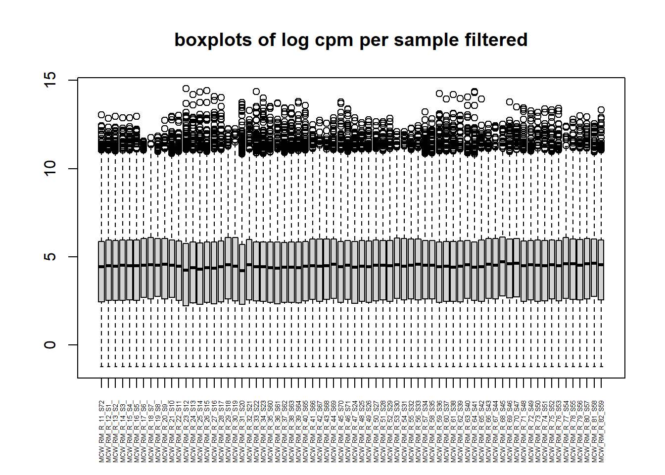
dim(x)[1] 14823 72write.csv(x$counts, "data/norm_counts.csv")Both of the above methods leave 14823 genes from 28,395. I prefer the second method, which keeps the DGEList format of the data.
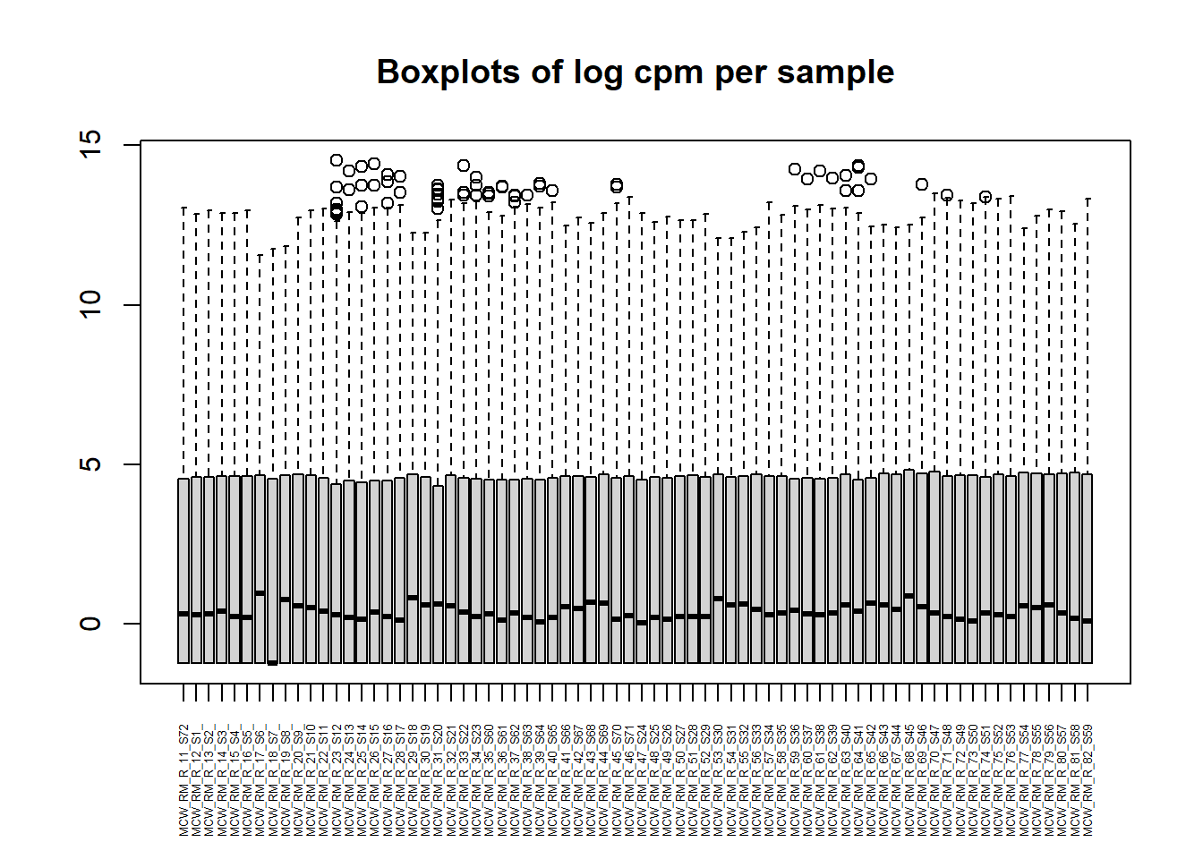
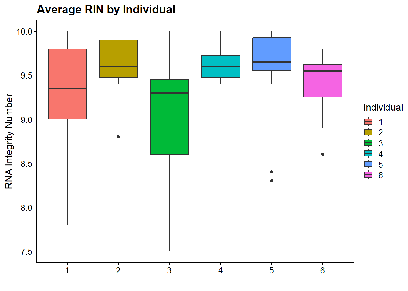
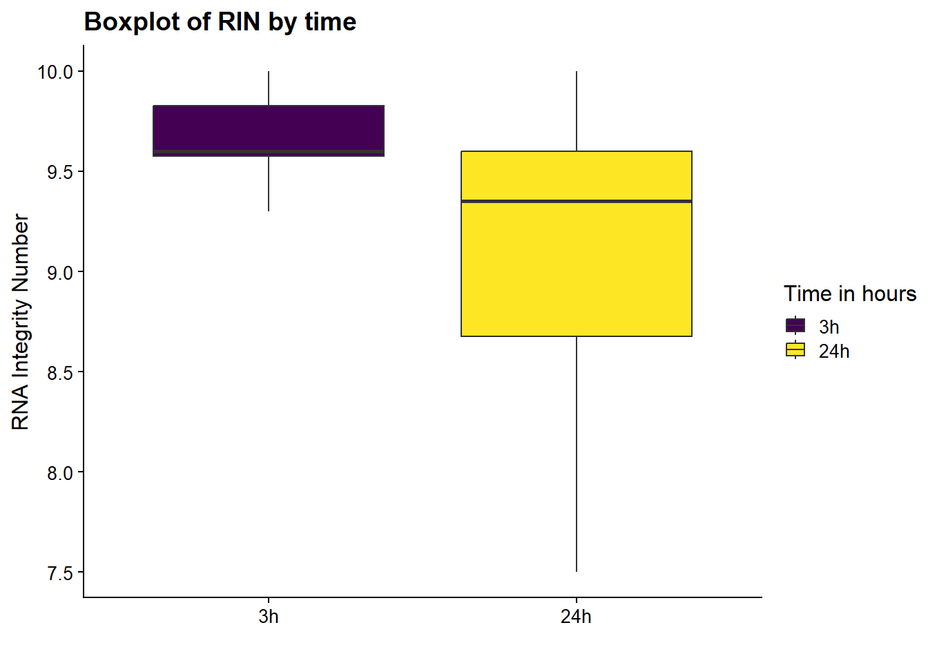
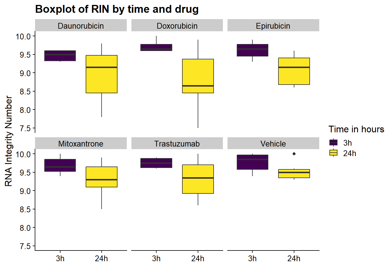
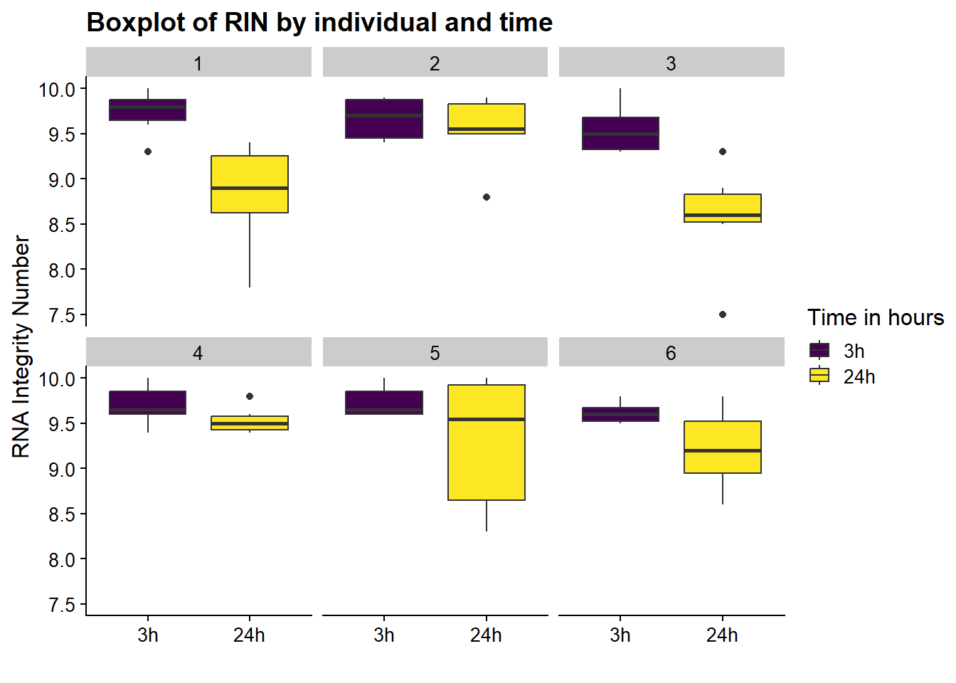
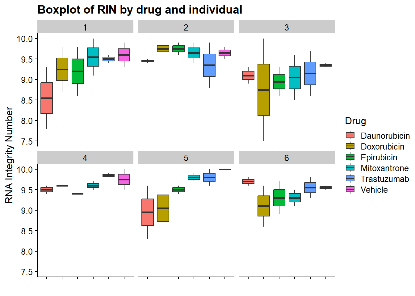
now I will produce the RIN x sample plots:###
Principal Component Analysis
PCA was done using code adopted from J. Blischak.
### Daunorubicin 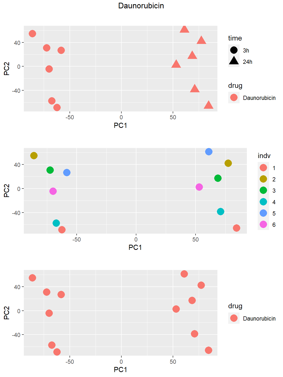
### Doxorubicin 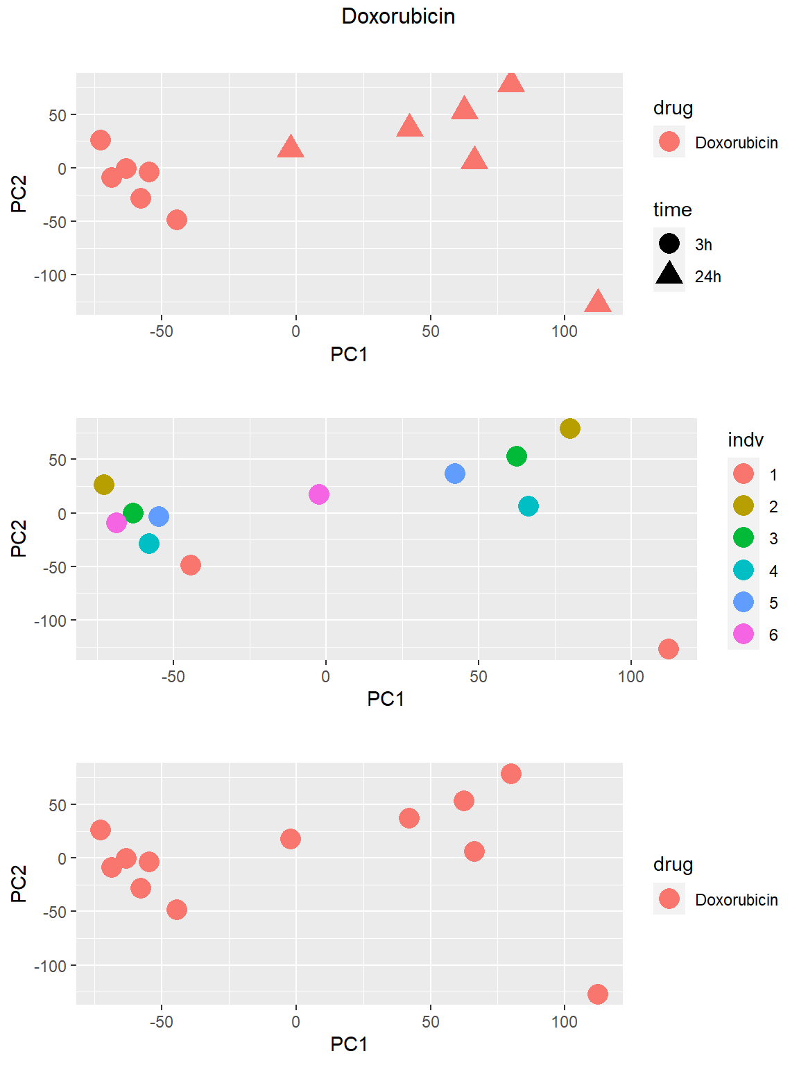
### Epirubicin 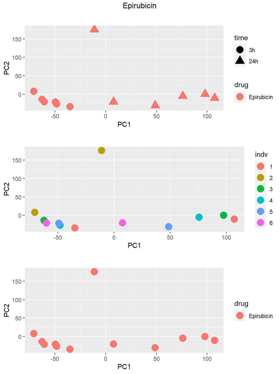
### Mitoxantrone 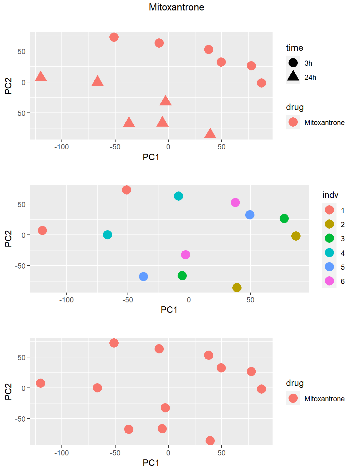
### Trastuzumab 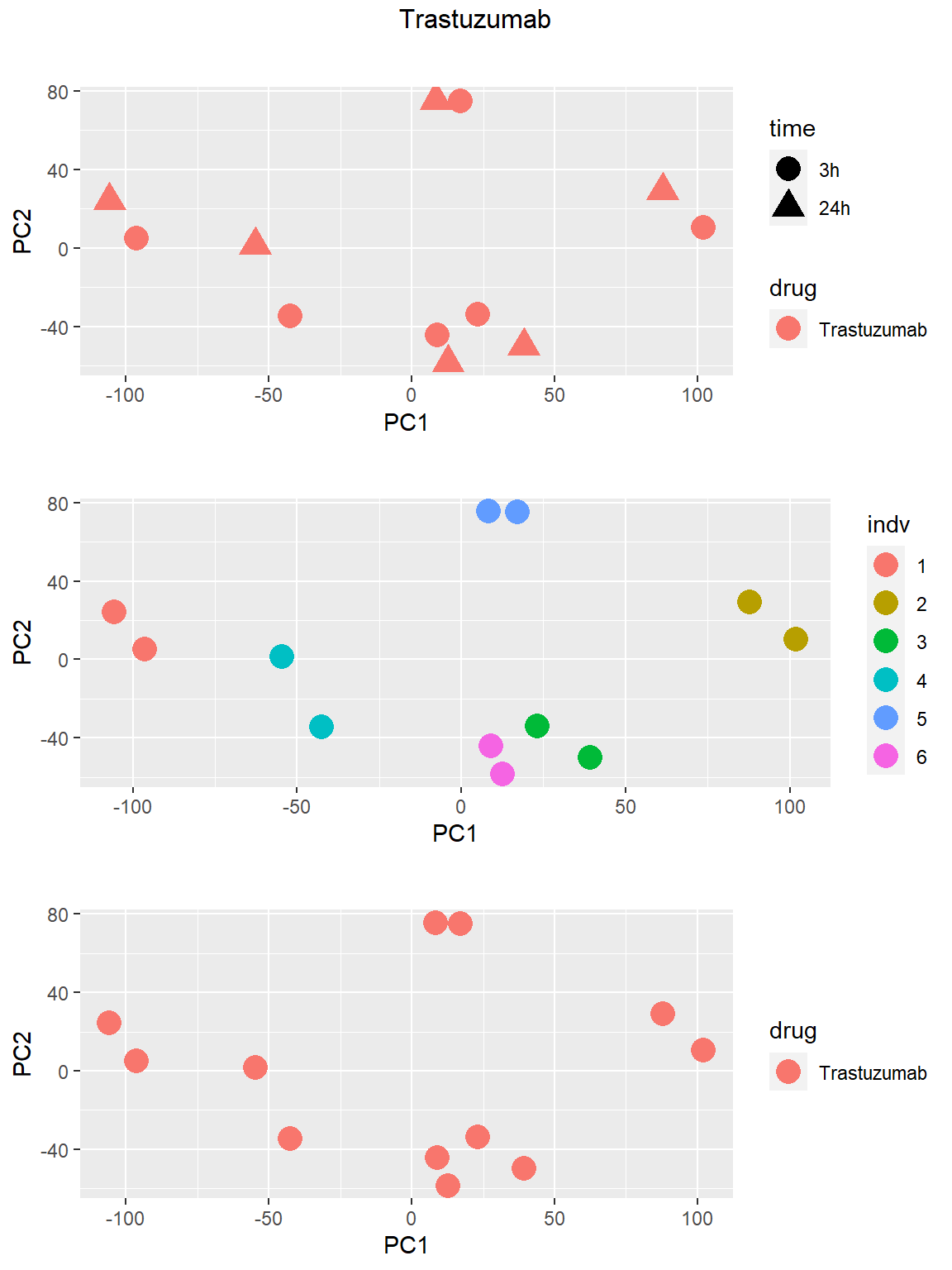
### Vehicle 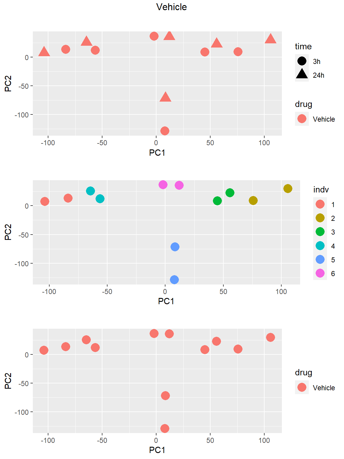
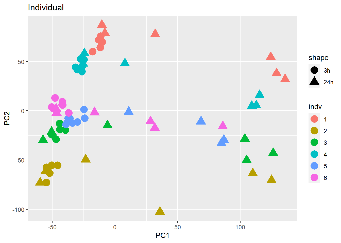
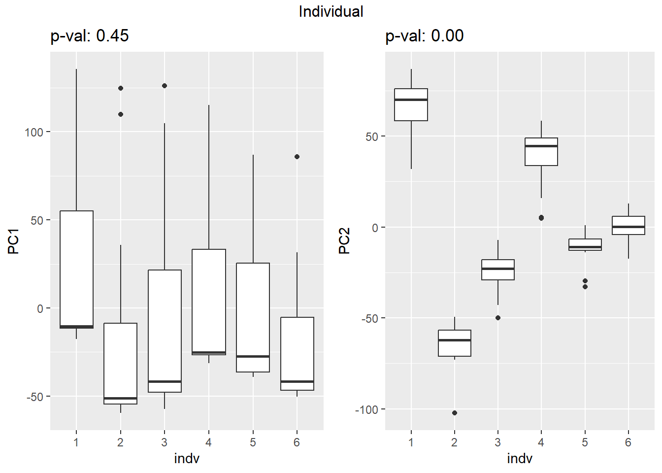
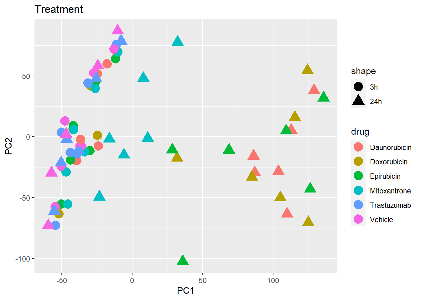
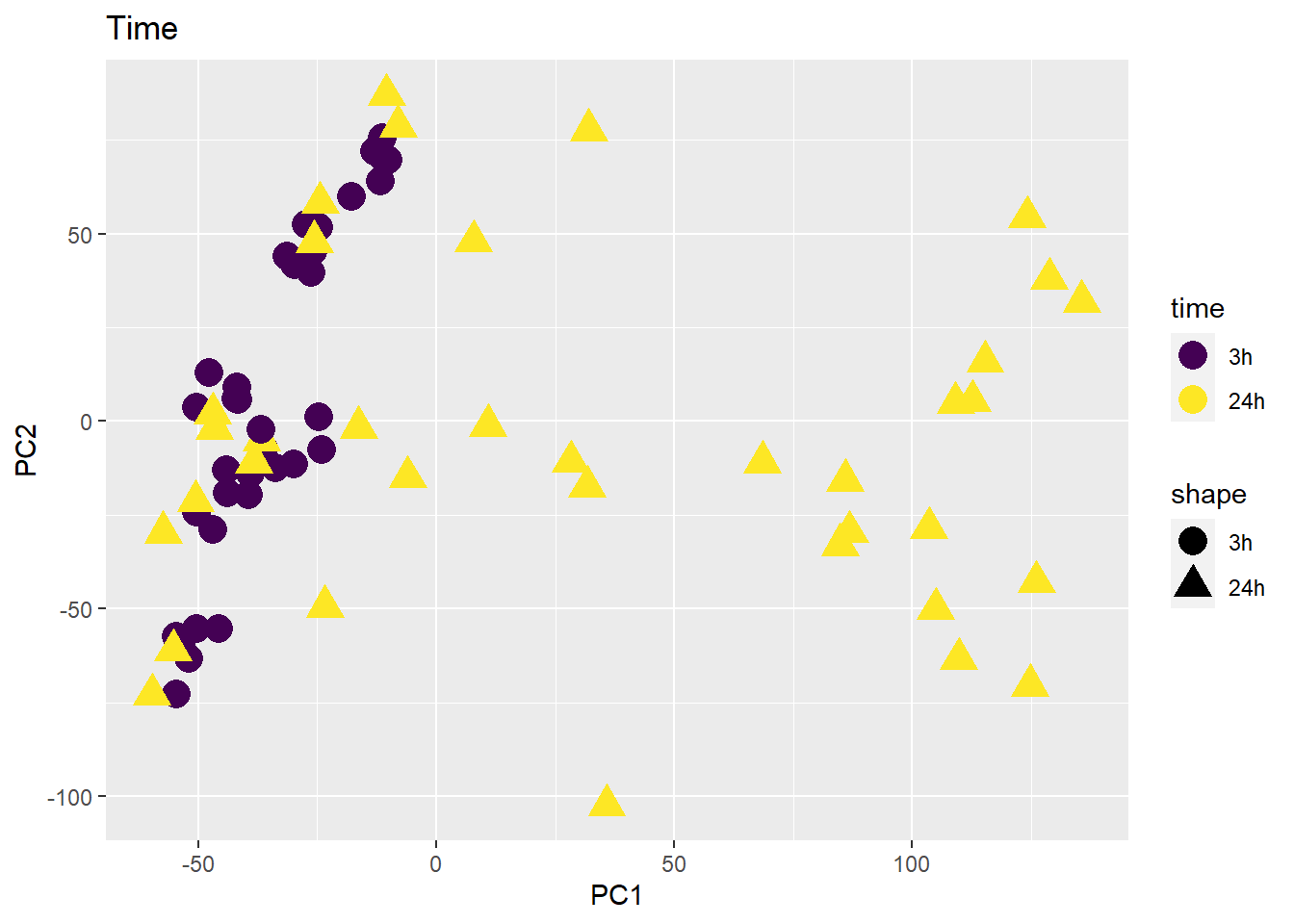
PCA of all 72 samples
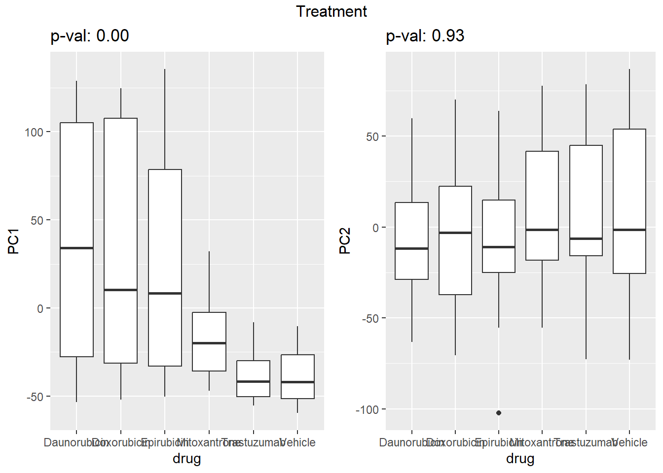
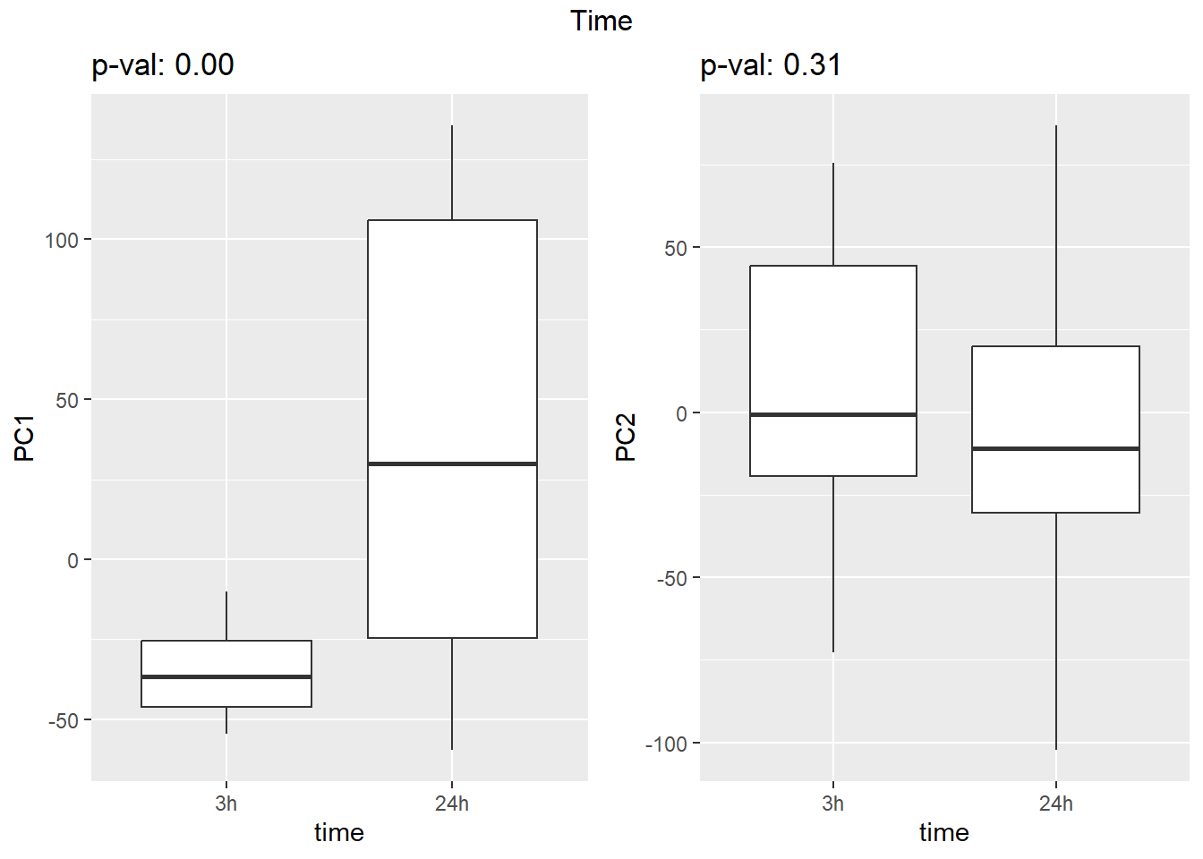
Warning: `qplot()` was deprecated in ggplot2 3.4.0.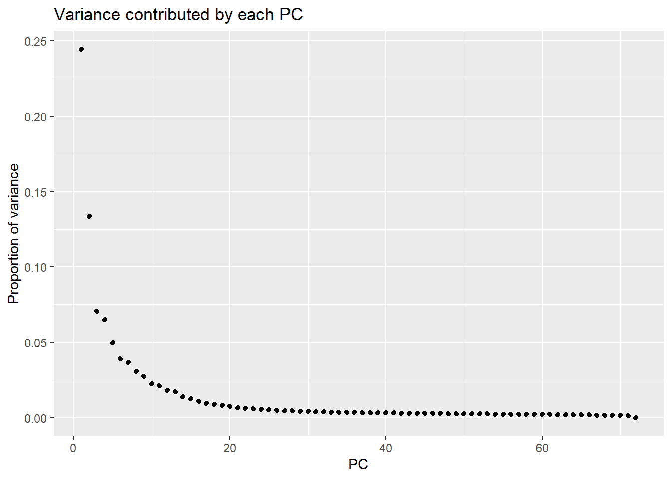 ## Variance contribution from treatment, extraction time, or individual
on PC1 and PC2
## Variance contribution from treatment, extraction time, or individual
on PC1 and PC2
Differential Expression
mm2 <- model.matrix(~0 + group1)
##made the matrix model using the interaction between Treatment and Time
colnames(mm2) <- c("A3", "X3", "E3","M3","T3", "V3","A24", "X24", "E24","M24","T24", "V24")
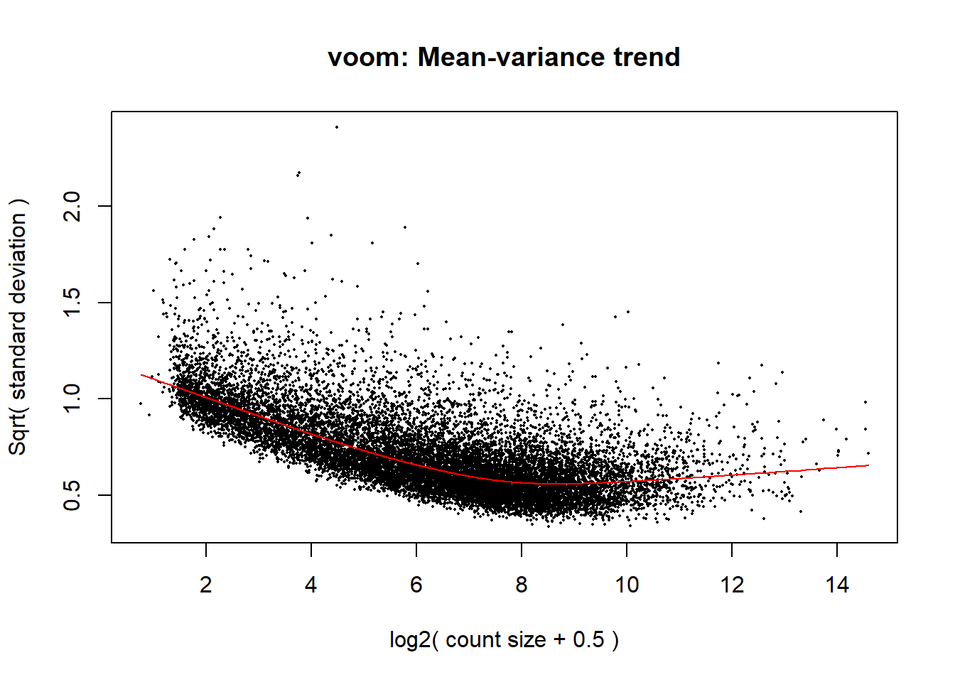
y2 <- voom(x, mm2)
corfit2 <- duplicateCorrelation(y2, mm2, block = indv)
v2 <- voom(x, mm2, block = indv, correlation = corfit2$consensus)
fit2 <- lmFit(v2, mm2, block = indv, correlation = corfit2$consensus)
vfit2 <- lmFit(y2, mm2)
vfit2<- contrasts.fit(vfit2, contrasts=cm2)
efit2 <- eBayes(vfit2)
V.DA.top= topTable(efit2, coef=1, adjust="BH", number=Inf, sort.by="p")
### sorting all top expressed genes for the Vehicle and Daunorubicin 3 hour treatments
sigVDA3 = V.DA.top[V.DA.top$adj.P.Val < .1 , ]
### this helped pull only those files that were at an adjusted p value of less than 0.1
### This p-value was used as the beginning examination of the data, considering I will run multiple runs of this RNA seq library.This is the example code I used to process my data. I used two model matrix initially, one set up was /~0 +drug +time and the second was /~0+group1, then blocking by individual. That is why you see the number 2 in the code above.
#DEG summary
Importance of components:
                           PC1     PC2     PC3      PC4     PC5      PC6
Standard deviation     60.2067 44.5108 32.3037 30.98489 27.1431 24.07762
Proportion of Variance  0.2445  0.1337  0.0704  0.06477  0.0497  0.03911
Cumulative Proportion   0.2445  0.3782  0.4486  0.51337  0.5631  0.60218
                            PC7      PC8      PC9     PC10     PC11     PC12
Standard deviation     23.26775 21.37712 20.13091 18.19509 17.63059 16.30004
Proportion of Variance  0.03652  0.03083  0.02734  0.02233  0.02097  0.01792
Cumulative Proportion   0.63870  0.66953  0.69687  0.71921  0.74018  0.75810
                           PC13     PC14     PC15     PC16     PC17     PC18
Standard deviation     15.87695 14.24554 13.51806 12.67177 11.84085 11.44481
Proportion of Variance  0.01701  0.01369  0.01233  0.01083  0.00946  0.00884
Cumulative Proportion   0.77511  0.78880  0.80113  0.81196  0.82142  0.83025
                           PC19    PC20    PC21    PC22    PC23    PC24    PC25
Standard deviation     11.08484 10.4711 9.86347 9.53287 9.25138 9.06027 8.70778
Proportion of Variance  0.00829  0.0074 0.00656 0.00613 0.00577 0.00554 0.00512
Cumulative Proportion   0.83854  0.8459 0.85250 0.85863 0.86441 0.86995 0.87506
                          PC26    PC27    PC28    PC29    PC30    PC31    PC32
Standard deviation     8.40220 8.26732 8.04037 7.85926 7.76676 7.67958 7.48930
Proportion of Variance 0.00476 0.00461 0.00436 0.00417 0.00407 0.00398 0.00378
Cumulative Proportion  0.87982 0.88444 0.88880 0.89296 0.89703 0.90101 0.90480
                          PC33    PC34    PC35   PC36    PC37    PC38    PC39
Standard deviation     7.34178 7.28566 7.22861 7.1043 6.99972 6.94542 6.83650
Proportion of Variance 0.00364 0.00358 0.00353 0.0034 0.00331 0.00325 0.00315
Cumulative Proportion  0.90843 0.91201 0.91554 0.9189 0.92225 0.92550 0.92866
                          PC40    PC41    PC42    PC43    PC44   PC45    PC46
Standard deviation     6.75717 6.73038 6.57835 6.54307 6.53123 6.4395 6.37432
Proportion of Variance 0.00308 0.00306 0.00292 0.00289 0.00288 0.0028 0.00274
Cumulative Proportion  0.93174 0.93479 0.93771 0.94060 0.94348 0.9463 0.94902
                          PC47    PC48    PC49   PC50    PC51   PC52    PC53
Standard deviation     6.34772 6.23190 6.17748 6.0816 6.01946 5.9644 5.89730
Proportion of Variance 0.00272 0.00262 0.00257 0.0025 0.00244 0.0024 0.00235
Cumulative Proportion  0.95173 0.95435 0.95693 0.9594 0.96187 0.9643 0.96661
                         PC54    PC55    PC56    PC57    PC58    PC59    PC60
Standard deviation     5.8378 5.80173 5.72099 5.69367 5.65008 5.60128 5.47568
Proportion of Variance 0.0023 0.00227 0.00221 0.00219 0.00215 0.00212 0.00202
Cumulative Proportion  0.9689 0.97118 0.97339 0.97558 0.97773 0.97985 0.98187
                          PC61    PC62    PC63    PC64    PC65   PC66    PC67
Standard deviation     5.46660 5.38710 5.31872 5.25710 5.11760 5.0166 4.83245
Proportion of Variance 0.00202 0.00196 0.00191 0.00186 0.00177 0.0017 0.00158
Cumulative Proportion  0.98389 0.98585 0.98776 0.98962 0.99139 0.9931 0.99466
                          PC68    PC69    PC70    PC71      PC72
Standard deviation     4.73475 4.57831 4.51242 3.92680 4.923e-14
Proportion of Variance 0.00151 0.00141 0.00137 0.00104 0.000e+00
Cumulative Proportion  0.99617 0.99759 0.99896 1.00000 1.000e+00
V.DA V.DX V.EP V.MT V.TR V.DA24 V.DX24 V.EP24 V.MT24 V.TR24
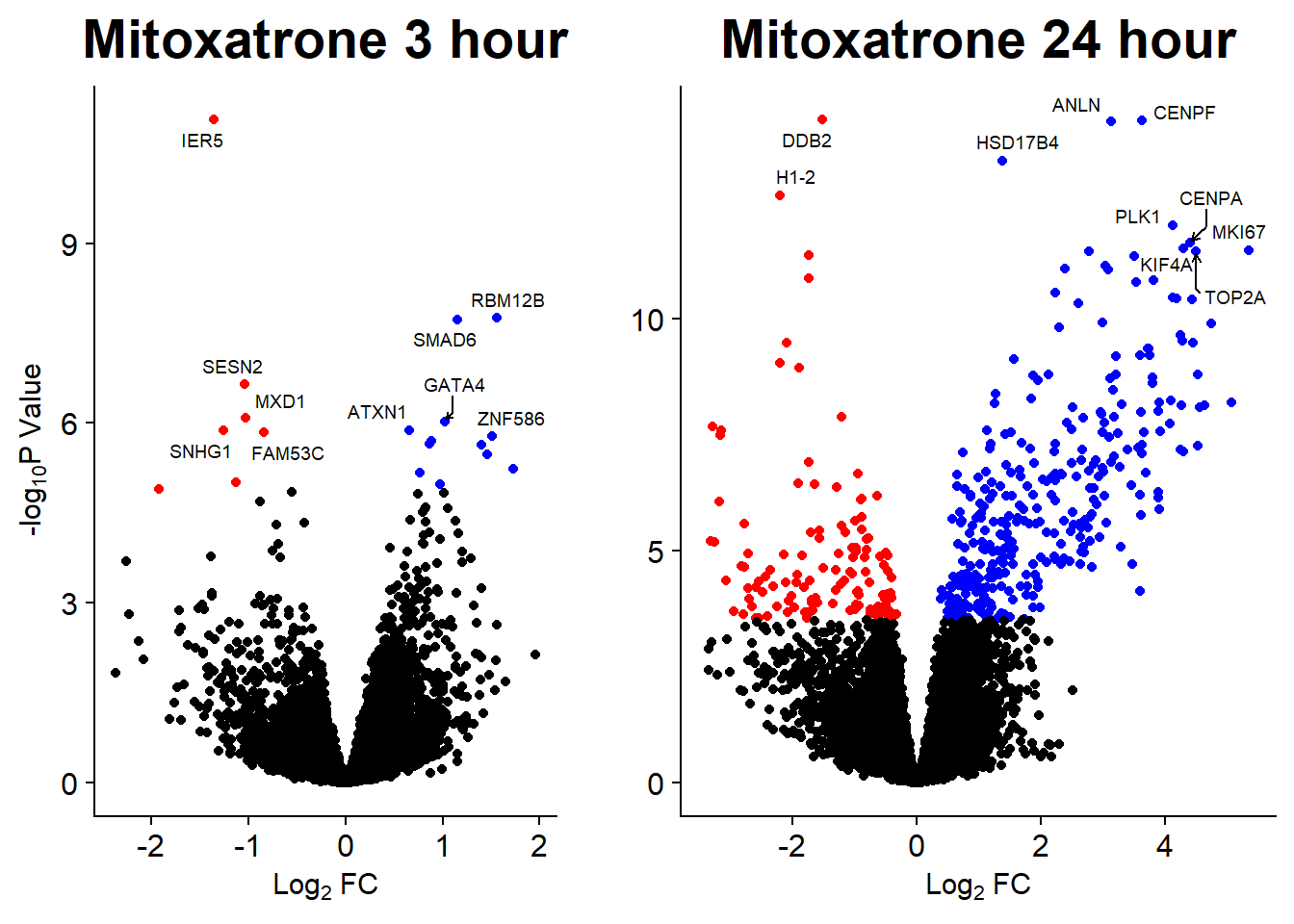
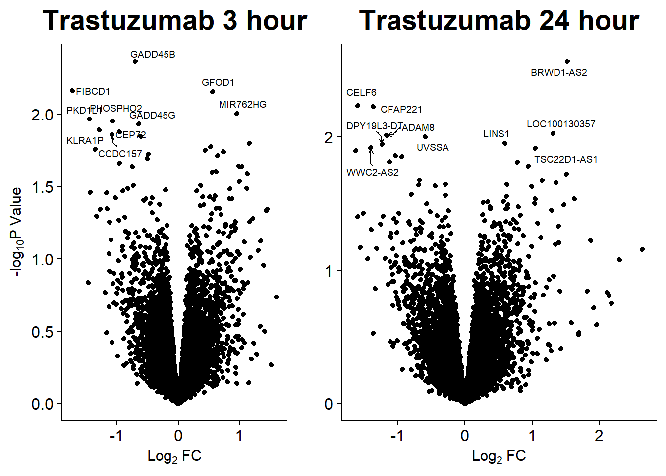
Down 63 3 11 13 0 3342 3013 2871 320 0
NotSig 14456 14814 14714 14780 14823 8279 8993 9034 13970 14823
Up 304 6 98 30 0 3202 2817 2918 533 0Graphing DE genes
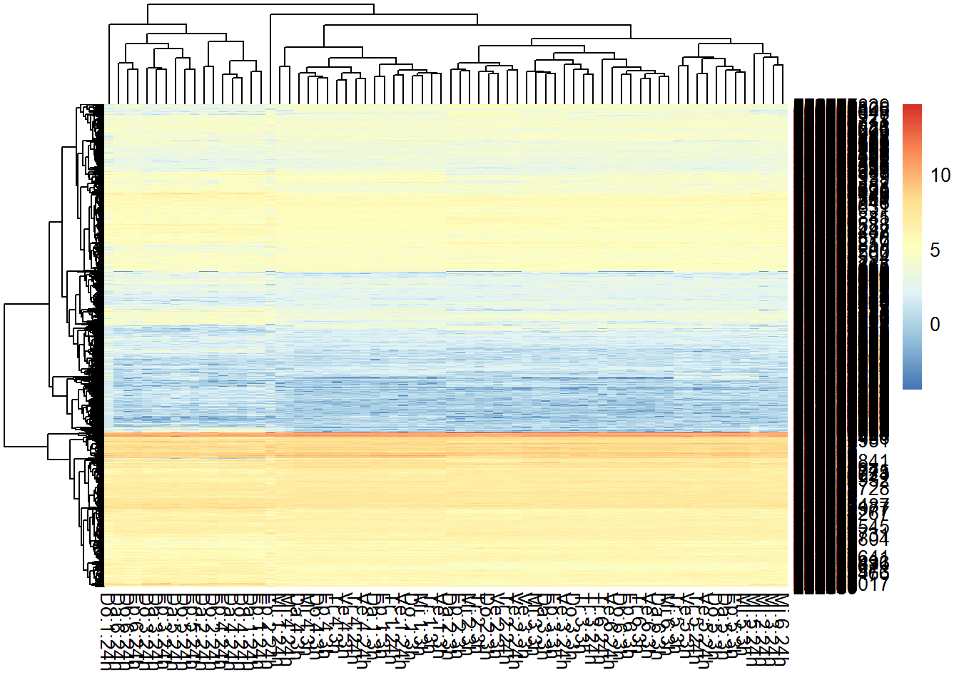
I then created a counts table for each set of genes. Luckily, the counts are stored in the y2 object, which is an EList class object. I can ‘simplify’ this process because I kept the DEGList format initially. I first made an object called ‘countstotal’ from the EList y2. For ggploting later, I subsetted ‘countstotal’ by treatments.
countstotal <- y2$E
colnames(countstotal) <- smlabel
boxplot(countstotal, xaxt = "n", xlab="")
Da3counts <- as.data.frame(as.table(countstotal[,c(1,6,13,18,25,30,37,42,49,54,61,66)]))
x_axis_labels(labels = label, every_nth = 1, adj=1, srt =90, cex =0.4)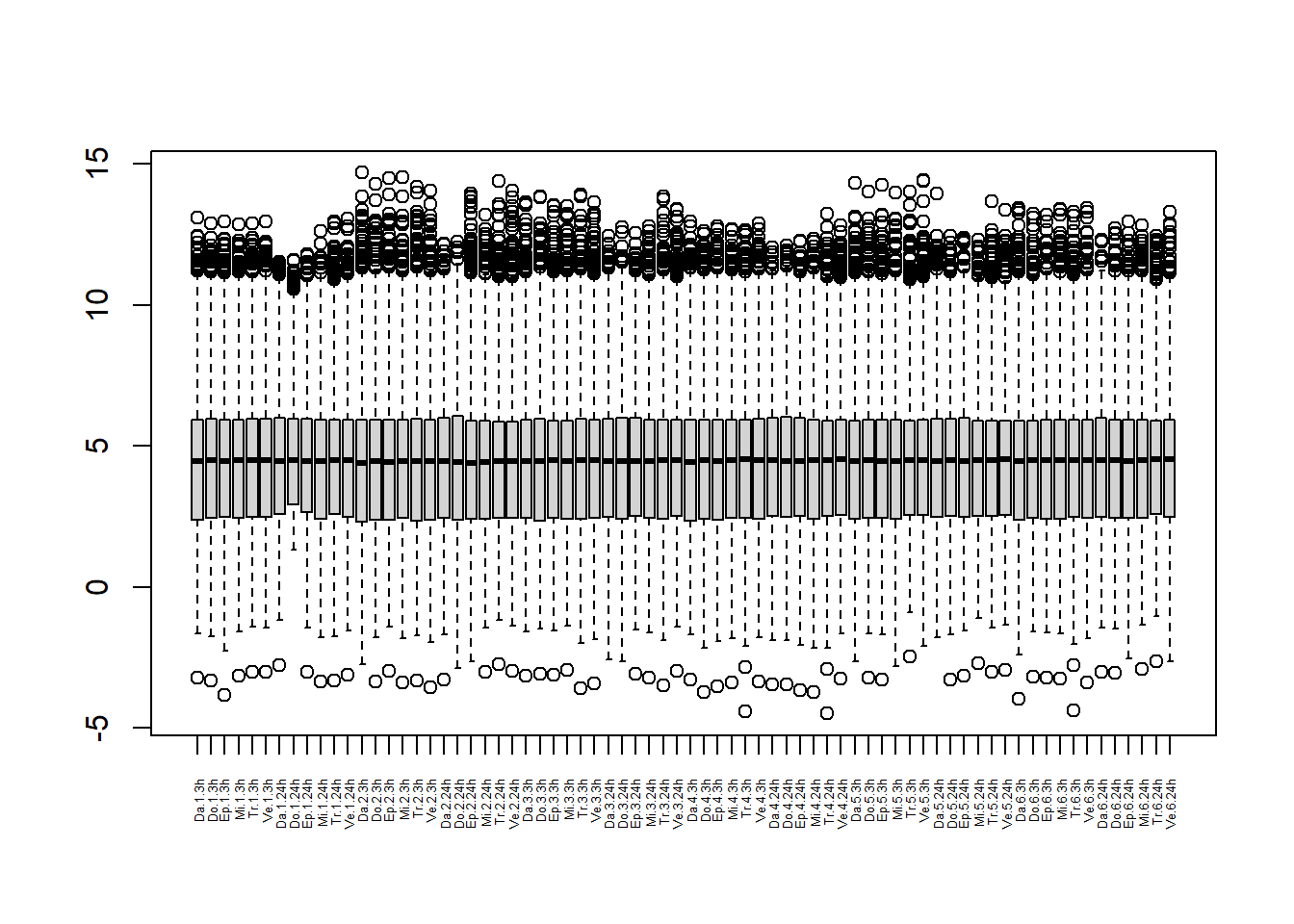
library(cowplot)
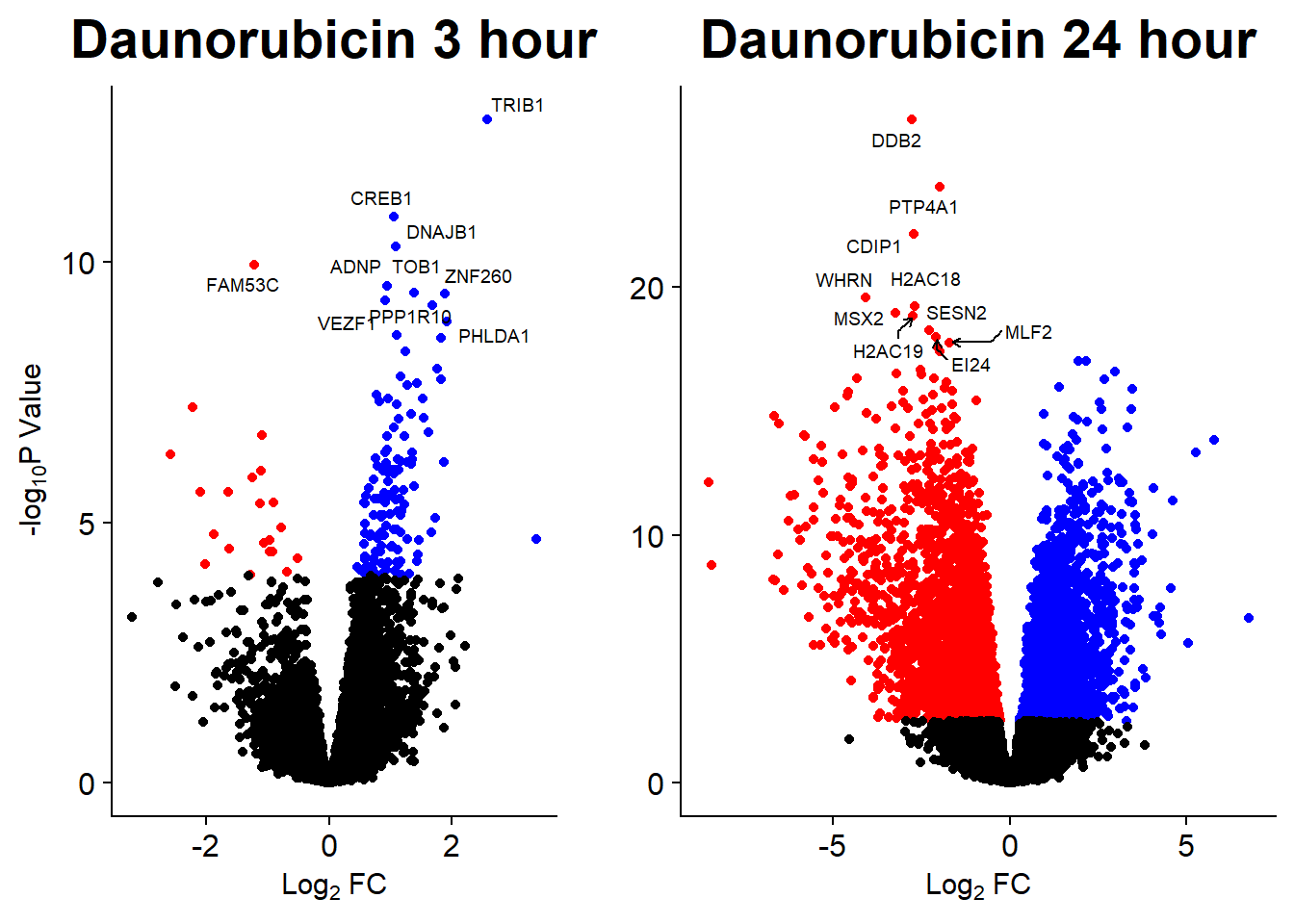
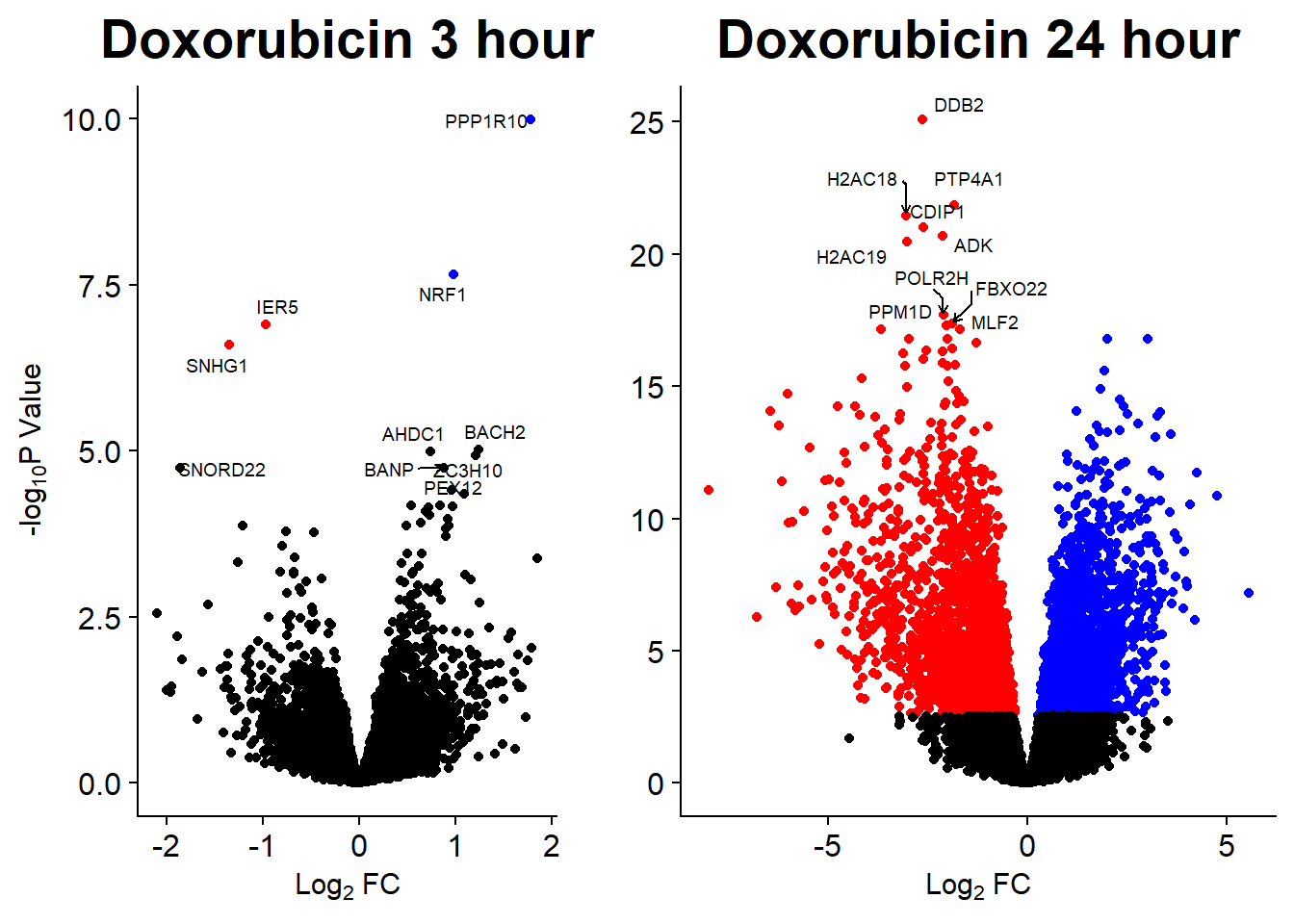
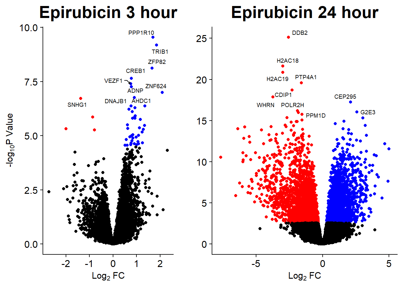
Volcano Plots
GO analysis
sessionInfo()R version 4.2.2 (2022-10-31 ucrt)
Platform: x86_64-w64-mingw32/x64 (64-bit)
Running under: Windows 10 x64 (build 19044)
Matrix products: default
locale:
[1] LC_COLLATE=English_United States.utf8
[2] LC_CTYPE=English_United States.utf8
[3] LC_MONETARY=English_United States.utf8
[4] LC_NUMERIC=C
[5] LC_TIME=English_United States.utf8
attached base packages:
[1] stats4 grid stats graphics grDevices utils datasets
[8] methods base
other attached packages:
[1] pheatmap_1.0.12
[2] Cormotif_1.42.0
[3] affy_1.74.0
[4] Hmisc_4.7-2
[5] Formula_1.2-4
[6] survival_3.5-0
[7] corrplot_0.92
[8] ggrepel_0.9.3
[9] cowplot_1.1.1
[10] Homo.sapiens_1.3.1
[11] TxDb.Hsapiens.UCSC.hg19.knownGene_3.2.2
[12] org.Hs.eg.db_3.15.0
[13] GO.db_3.15.0
[14] OrganismDbi_1.38.1
[15] GenomicFeatures_1.48.4
[16] GenomicRanges_1.48.0
[17] GenomeInfoDb_1.32.4
[18] AnnotationDbi_1.58.0
[19] IRanges_2.30.1
[20] S4Vectors_0.34.0
[21] biomaRt_2.52.0
[22] scales_1.2.1
[23] forcats_1.0.0
[24] stringr_1.5.0
[25] dplyr_1.1.0
[26] purrr_1.0.1
[27] readr_2.1.3
[28] tidyr_1.3.0
[29] tibble_3.1.8
[30] tidyverse_1.3.2
[31] AnnotationHub_3.4.0
[32] BiocFileCache_2.4.0
[33] dbplyr_2.3.0
[34] devtools_2.4.5
[35] usethis_2.1.6
[36] reshape2_1.4.4
[37] gridExtra_2.3
[38] HTSFilter_1.36.0
[39] VennDiagram_1.7.3
[40] futile.logger_1.4.3
[41] mixOmics_6.20.0
[42] ggplot2_3.4.0
[43] lattice_0.20-45
[44] MASS_7.3-58.2
[45] RColorBrewer_1.1-3
[46] edgeR_3.38.4
[47] limma_3.52.4
[48] Biobase_2.56.0
[49] BiocGenerics_0.42.0
[50] workflowr_1.7.0
loaded via a namespace (and not attached):
[1] rappdirs_0.3.3 rtracklayer_1.56.1
[3] bit64_4.0.5 knitr_1.42
[5] DelayedArray_0.22.0 data.table_1.14.6
[7] rpart_4.1.19 KEGGREST_1.36.3
[9] RCurl_1.98-1.10 generics_0.1.3
[11] preprocessCore_1.58.0 callr_3.7.3
[13] lambda.r_1.2.4 RSQLite_2.2.20
[15] bit_4.0.5 tzdb_0.3.0
[17] xml2_1.3.3 lubridate_1.9.1
[19] httpuv_1.6.8 SummarizedExperiment_1.26.1
[21] assertthat_0.2.1 gargle_1.3.0
[23] xfun_0.37 hms_1.1.2
[25] jquerylib_0.1.4 evaluate_0.20
[27] promises_1.2.0.1 fansi_1.0.4
[29] restfulr_0.0.15 progress_1.2.2
[31] readxl_1.4.1 igraph_1.3.5
[33] DBI_1.1.3 geneplotter_1.74.0
[35] htmlwidgets_1.6.1 rARPACK_0.11-0
[37] googledrive_2.0.0 ellipsis_0.3.2
[39] RSpectra_0.16-1 backports_1.4.1
[41] annotate_1.74.0 deldir_1.0-6
[43] MatrixGenerics_1.8.1 vctrs_0.5.2
[45] remotes_2.4.2 cachem_1.0.6
[47] withr_2.5.0 checkmate_2.1.0
[49] GenomicAlignments_1.32.1 prettyunits_1.1.1
[51] cluster_2.1.4 crayon_1.5.2
[53] ellipse_0.4.3 genefilter_1.78.0
[55] pkgconfig_2.0.3 labeling_0.4.2
[57] pkgload_1.3.2 nnet_7.3-18
[59] rlang_1.0.6 lifecycle_1.0.3
[61] miniUI_0.1.1.1 filelock_1.0.2
[63] affyio_1.66.0 modelr_0.1.10
[65] cellranger_1.1.0 rprojroot_2.0.3
[67] matrixStats_0.63.0 graph_1.74.0
[69] Matrix_1.5-3 reprex_2.0.2
[71] base64enc_0.1-3 whisker_0.4.1
[73] processx_3.8.0 googlesheets4_1.0.1
[75] png_0.1-8 viridisLite_0.4.1
[77] rjson_0.2.21 bitops_1.0-7
[79] getPass_0.2-2 Biostrings_2.64.1
[81] blob_1.2.3 jpeg_0.1-10
[83] memoise_2.0.1 magrittr_2.0.3
[85] plyr_1.8.8 zlibbioc_1.42.0
[87] compiler_4.2.2 BiocIO_1.6.0
[89] DESeq2_1.36.0 Rsamtools_2.12.0
[91] cli_3.6.0 XVector_0.36.0
[93] urlchecker_1.0.1 ps_1.7.2
[95] htmlTable_2.4.1 formatR_1.14
[97] tidyselect_1.2.0 stringi_1.7.12
[99] highr_0.10 yaml_2.3.7
[101] locfit_1.5-9.7 latticeExtra_0.6-30
[103] sass_0.4.5 tools_4.2.2
[105] timechange_0.2.0 parallel_4.2.2
[107] rstudioapi_0.14 foreign_0.8-84
[109] git2r_0.31.0 farver_2.1.1
[111] digest_0.6.31 BiocManager_1.30.19
[113] shiny_1.7.4 Rcpp_1.0.10
[115] broom_1.0.3 BiocVersion_3.15.2
[117] later_1.3.0 httr_1.4.4
[119] colorspace_2.1-0 rvest_1.0.3
[121] XML_3.99-0.13 fs_1.6.1
[123] splines_4.2.2 RBGL_1.72.0
[125] statmod_1.5.0 sessioninfo_1.2.2
[127] xtable_1.8-4 jsonlite_1.8.4
[129] futile.options_1.0.1 corpcor_1.6.10
[131] R6_2.5.1 profvis_0.3.7
[133] pillar_1.8.1 htmltools_0.5.4
[135] mime_0.12 glue_1.6.2
[137] fastmap_1.1.0 BiocParallel_1.30.4
[139] interactiveDisplayBase_1.34.0 codetools_0.2-19
[141] pkgbuild_1.4.0 utf8_1.2.3
[143] bslib_0.4.2 curl_5.0.0
[145] interp_1.1-3 rmarkdown_2.20
[147] munsell_0.5.0 GenomeInfoDbData_1.2.8
[149] haven_2.5.1 gtable_0.3.1