ATAC_fastqc
ERM
2024-02-19
Last updated: 2024-02-19
Checks: 7 0
Knit directory: ATAC_learning/
This reproducible R Markdown analysis was created with workflowr (version 1.7.1). The Checks tab describes the reproducibility checks that were applied when the results were created. The Past versions tab lists the development history.
Great! Since the R Markdown file has been committed to the Git repository, you know the exact version of the code that produced these results.
Great job! The global environment was empty. Objects defined in the global environment can affect the analysis in your R Markdown file in unknown ways. For reproduciblity it’s best to always run the code in an empty environment.
The command set.seed(20231016) was run prior to running
the code in the R Markdown file. Setting a seed ensures that any results
that rely on randomness, e.g. subsampling or permutations, are
reproducible.
Great job! Recording the operating system, R version, and package versions is critical for reproducibility.
Nice! There were no cached chunks for this analysis, so you can be confident that you successfully produced the results during this run.
Great job! Using relative paths to the files within your workflowr project makes it easier to run your code on other machines.
Great! You are using Git for version control. Tracking code development and connecting the code version to the results is critical for reproducibility.
The results in this page were generated with repository version 82d757c. See the Past versions tab to see a history of the changes made to the R Markdown and HTML files.
Note that you need to be careful to ensure that all relevant files for
the analysis have been committed to Git prior to generating the results
(you can use wflow_publish or
wflow_git_commit). workflowr only checks the R Markdown
file, but you know if there are other scripts or data files that it
depends on. Below is the status of the Git repository when the results
were generated:
Ignored files:
    Ignored:    .Rhistory
    Ignored:    .Rproj.user/
    Ignored:    data/Ind1_75DA24h_dedup_peaks.csv
    Ignored:    data/Ind4_79B24h_dedup_peaks.csv
    Ignored:    data/aln_run1_results.txt
    Ignored:    data/initial_complete_stats_run1.txt
    Ignored:    data/multiqc_fastqc_run1.txt
    Ignored:    data/multiqc_fastqc_run2.txt
    Ignored:    data/multiqc_genestat_run1.txt
    Ignored:    data/multiqc_genestat_run2.txt
    Ignored:    data/trimmed_seq_length.csv

Untracked files:
    Untracked:  code/just_for_Fun.R
Note that any generated files, e.g. HTML, png, CSS, etc., are not included in this status report because it is ok for generated content to have uncommitted changes.
These are the previous versions of the repository in which changes were
made to the R Markdown (analysis/Fastqc_results.Rmd) and
HTML (docs/Fastqc_results.html) files. If you’ve configured
a remote Git repository (see ?wflow_git_remote), click on
the hyperlinks in the table below to view the files as they were in that
past version.
| File | Version | Author | Date | Message |
|---|---|---|---|---|
| Rmd | 82d757c | reneeisnowhere | 2024-02-19 | adding in fragment length |
| html | 3e9762b | reneeisnowhere | 2024-01-30 | Build site. |
| Rmd | 778ce47 | reneeisnowhere | 2024-01-30 | adding more graphs |
| html | dce7d59 | reneeisnowhere | 2024-01-30 | Build site. |
| html | 83c0d79 | reneeisnowhere | 2024-01-30 | Build site. |
| Rmd | ccb3f28 | reneeisnowhere | 2024-01-30 | first updates |
library(tidyverse)
# library(ggsignif)
# library(cowplot)
# library(ggpubr)
# library(scales)
# library(sjmisc)
library(kableExtra)
# library(broom)
# library(biomaRt)
library(RColorBrewer)
# library(gprofiler2)
# library(qvalue)
Total Sequences
This code takes the multiqc fastqc output file and: splits by rows to trimmed and non trimmed, then separates the trimmed file names into catagories I want, then adds back in the non trimmed data rows (while also splitting file name like the trimmed file name). after rbind, I split treatmenttime by position, fix the names of the time column, remove numbers from trt column, add a new column called “trimmed” where I add in a vector that lets me group by trimmed file verses non trimmed file, the select only those columns containing the columns I want to keep.
multiqc_fastqc2 <- read_csv("data/multiqc_fastqc_run2.txt")
multiqc_general_stats2 <- read_csv("data/multiqc_genestat_run2.txt")


fastqc_full <- multiqc_fastqc2 %>%
  slice_tail(n=144) %>%
  separate(Filename, into = c(NA,"ind","treatmenttime",NA,"read")) %>%
  rbind(., (multiqc_fastqc2 %>% slice_head(n=144) %>% separate(Filename, into = c("ind","treatmenttime",NA,"read")))) %>%
  separate_wider_position(., col =treatmenttime,c(2,trt=2,time=3),too_few = "align_start") %>%
  mutate(time=case_match(trt,"E2"~"24h","E3"~"3h","M2"~"24h", "M3"~"3h","T2"~"24h","T3"~"3h","V2"~"24h","V3"~"3h",.default = time)) %>%
  mutate(trt=gsub("[[:digit:]]", "", trt) ) %>%
  mutate(trimmed = if_else(grepl(pattern ="^trim", x = Sample)==TRUE, "yes","no")) %>%
  select(Sample:read, trimmed,`Total Sequences`:avg_sequence_length) %>%
  full_join(., multiqc_general_stats2, join_by(Sample)) %>%
   rename("percent_gc"="FastQC_mqc-generalstats-fastqc-percent_gc",
         "avg_seq_len"= "FastQC_mqc-generalstats-fastqc-avg_sequence_length",
         "percent_dup"= "FastQC_mqc-generalstats-fastqc-percent_duplicates",
         "percent_fails"= "FastQC_mqc-generalstats-fastqc-percent_fails",
         "total_sequences"= "FastQC_mqc-generalstats-fastqc-total_sequences") %>%
  mutate(ind = factor(ind, levels = c("Ind1", "Ind2", "Ind3", "Ind4", "Ind5", "Ind6"))) %>%
  mutate(time = factor(time, levels = c("3h", "24h"), labels= c("3 hours","24 hours"))) %>%
  mutate(trt = factor(trt, levels = c("DX","E", "DA","M", "T", "V"), labels = c("DOX","EPI", "DNR", "MTX", "TRZ", "VEH")))
(in this case, Sample, ind, trt, time read, trimmed, Total sequences, Flagged poor quality, sequence length, %GC,total deduplicated %,and avg sequence length) I also then addin the gen_stats file and rename the columns to normal things.
fastqc_full# A tibble: 288 × 17
Sample ind trt time read trimmed `Total Sequences`
<chr> <fct> <fct> <fct> <chr> <chr> <dbl>
1 trimmed_Ind1_75DA24h_S7_R1 Ind1 DNR 24 ho… R1 yes 42551223
2 trimmed_Ind1_75DA24h_S7_R2 Ind1 DNR 24 ho… R2 yes 42551223
3 trimmed_Ind1_75DA3h_S1_R1 Ind1 DNR 3 hou… R1 yes 48230311
4 trimmed_Ind1_75DA3h_S1_R2 Ind1 DNR 3 hou… R2 yes 48230311
5 trimmed_Ind1_75DX24h_S8_R1 Ind1 DOX 24 ho… R1 yes 43284466
6 trimmed_Ind1_75DX24h_S8_R2 Ind1 DOX 24 ho… R2 yes 43284466
7 trimmed_Ind1_75DX3h_S2_R1 Ind1 DOX 3 hou… R1 yes 44480840
8 trimmed_Ind1_75DX3h_S2_R2 Ind1 DOX 3 hou… R2 yes 44480840
9 trimmed_Ind1_75E24h_S9_R1 Ind1 EPI 24 ho… R1 yes 42757767
10 trimmed_Ind1_75E24h_S9_R2 Ind1 EPI 24 ho… R2 yes 42757767
# ℹ 278 more rows
# ℹ 10 more variables: `Sequences flagged as poor quality` <dbl>,
# `Sequence length` <chr>, `%GC` <dbl>, total_deduplicated_percentage <dbl>,
# avg_sequence_length <dbl>, percent_dup <dbl>, percent_gc <dbl>,
# avg_seq_len <dbl>, percent_fails <dbl>, total_sequences <dbl>drug_pal <- c("#8B006D","#DF707E","#F1B72B", "#3386DD","#707031","#41B333")
fastqc_full %>%
filter(trimmed=="no") %>%
ggplot(., aes(x=trt, y= `Total Sequences`))+
geom_col(aes(fill= trt))+
facet_wrap(ind~time)+
scale_fill_manual(values=drug_pal)+
theme_bw()+
ggtitle("Total Sequences, untrimmed")+
# ylab(ylab)+
xlab("")+
theme(strip.background = element_rect(fill = "white",linetype=1, linewidth = 0.5),
plot.title = element_text(size=14,hjust = 0.5,face="bold"),
axis.title = element_text(size = 10, color = "black"),
axis.ticks = element_line(linewidth = 0.5),
axis.line = element_line(linewidth = 0.5),
axis.text.x = element_blank(),
strip.text.x = element_text(margin = margin(2,0,2,0, "pt"),face = "bold"))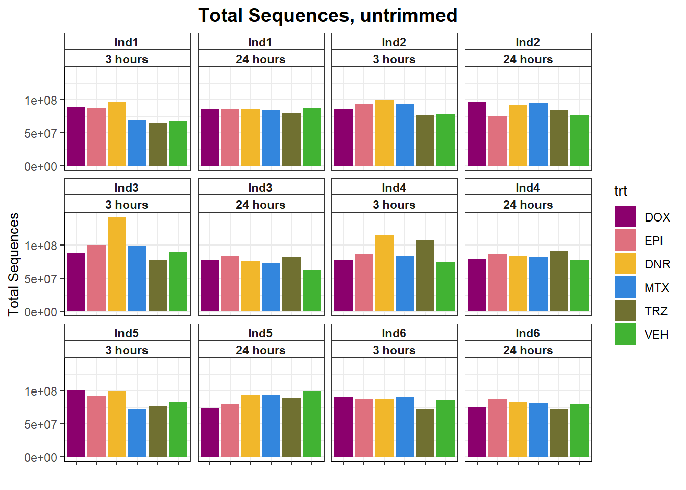
| Version | Author | Date |
|---|---|---|
| 83c0d79 | reneeisnowhere | 2024-01-30 |
fastqc_full %>%
  filter(trimmed=="yes") %>%
  ggplot(., aes(x=trt, y= `Total Sequences`))+
  geom_col(aes(fill= trt))+
  facet_wrap(ind~time)+
  scale_fill_manual(values=drug_pal)+
  theme_bw()+
  ggtitle("Total Sequences, trimmed")+
      # ylab(ylab)+
      xlab("")+
      theme(strip.background = element_rect(fill = "white",linetype=1, linewidth = 0.5),
          plot.title = element_text(size=14,hjust = 0.5,face="bold"),
          axis.title = element_text(size = 10, color = "black"),
          axis.ticks = element_line(linewidth = 0.5),
          axis.line = element_line(linewidth = 0.5),
          axis.text.x = element_blank(),
          strip.text.x = element_text(margin = margin(2,0,2,0, "pt"),face = "bold"))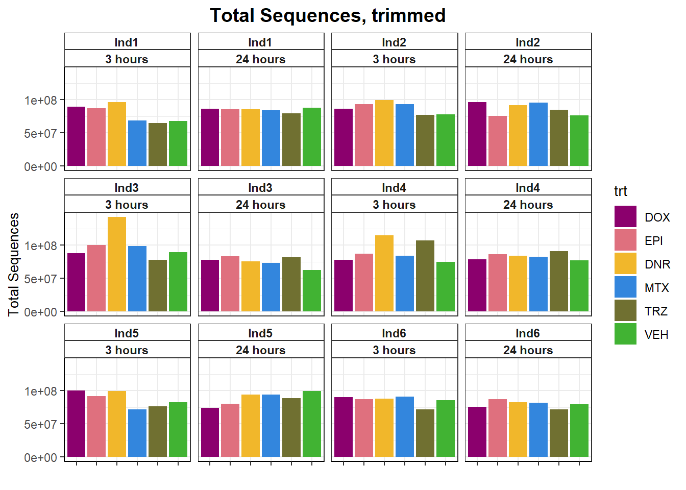
| Version | Author | Date |
|---|---|---|
| 83c0d79 | reneeisnowhere | 2024-01-30 |
totseq <- fastqc_full %>%
  dplyr::filter(read =='R1') %>%
  # group_by(ind,trt,time) %>%
 select(Sample, ind, trt, time, trimmed, `Total Sequences`) %>%
  pivot_wider(id_cols = c(ind,trt,time), names_from = trimmed, values_from = `Total Sequences`) %>%
  mutate(perc_removed=(no-yes)/no*100) #%>%
 kable(list(totseq[1:36,], totseq[37:72,]),caption= "Summary of Total sequences before and after trimming, with percentage of removed sequences") %>%
  kable_paper("striped", full_width = FALSE) %>%
  kable_styling(full_width = FALSE,font_size = 18) #%>%
|
|
   # scroll_box(width = "100%", height = "400px")

  totseq %>%
    ggplot(.,aes(x=trt,y=perc_removed) )+
    geom_col(aes(fill= trt))+
  facet_wrap(ind~time)+
  scale_fill_manual(values=drug_pal)+
  theme_bw()+
  ggtitle("Total Sequences, percent removed")+
      # ylab(ylab)+
      xlab("")+
      theme(strip.background = element_rect(fill = "white",linetype=1, linewidth = 0.5),
          plot.title = element_text(size=14,hjust = 0.5,face="bold"),
          axis.title = element_text(size = 10, color = "black"),
          axis.ticks = element_line(linewidth = 0.5),
          axis.line = element_line(linewidth = 0.5),
          axis.text.x = element_blank(),
          strip.text.x = element_text(margin = margin(2,0,2,0, "pt"),face = "bold"))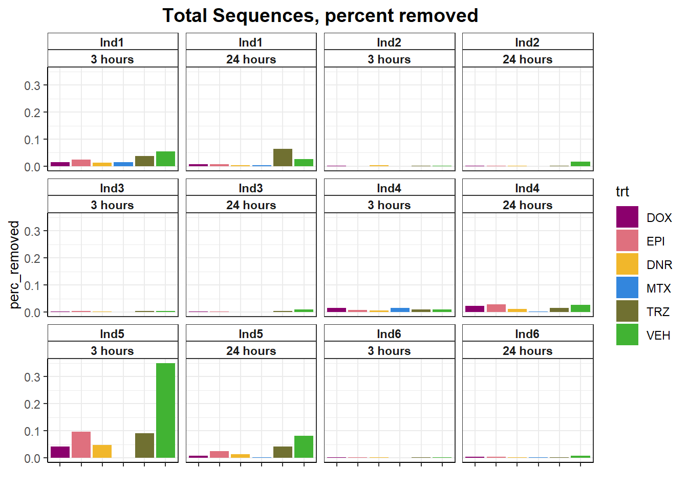
| Version | Author | Date |
|---|---|---|
| 83c0d79 | reneeisnowhere | 2024-01-30 |
##Average sequence length
fastqc_full %>%

  filter(trimmed=="no") %>%
  mutate(avg_sequence_length=as.numeric(avg_sequence_length)) %>%
  ggplot(., aes(x=read, y= avg_seq_len))+
  geom_boxplot(aes(fill= trt))+
  facet_wrap(ind~time)+
  scale_fill_manual(values=drug_pal)+
  theme_bw()+
  # ylim(0,55)+
  ggtitle("Average sequence length, untrimmed")+
      # ylab(ylab)+
      # xlab("")+
      theme(strip.background = element_rect(fill = "white",linetype=1, linewidth = 0.5),
          plot.title = element_text(size=14,hjust = 0.5,face="bold"),
          axis.title = element_text(size = 10, color = "black"),
          axis.ticks = element_line(linewidth = 0.5),
          axis.line = element_line(linewidth = 0.5),
          # axis.text.x = element_blank(),
          strip.text.x = element_text(margin = margin(2,0,2,0, "pt"),face = "bold"))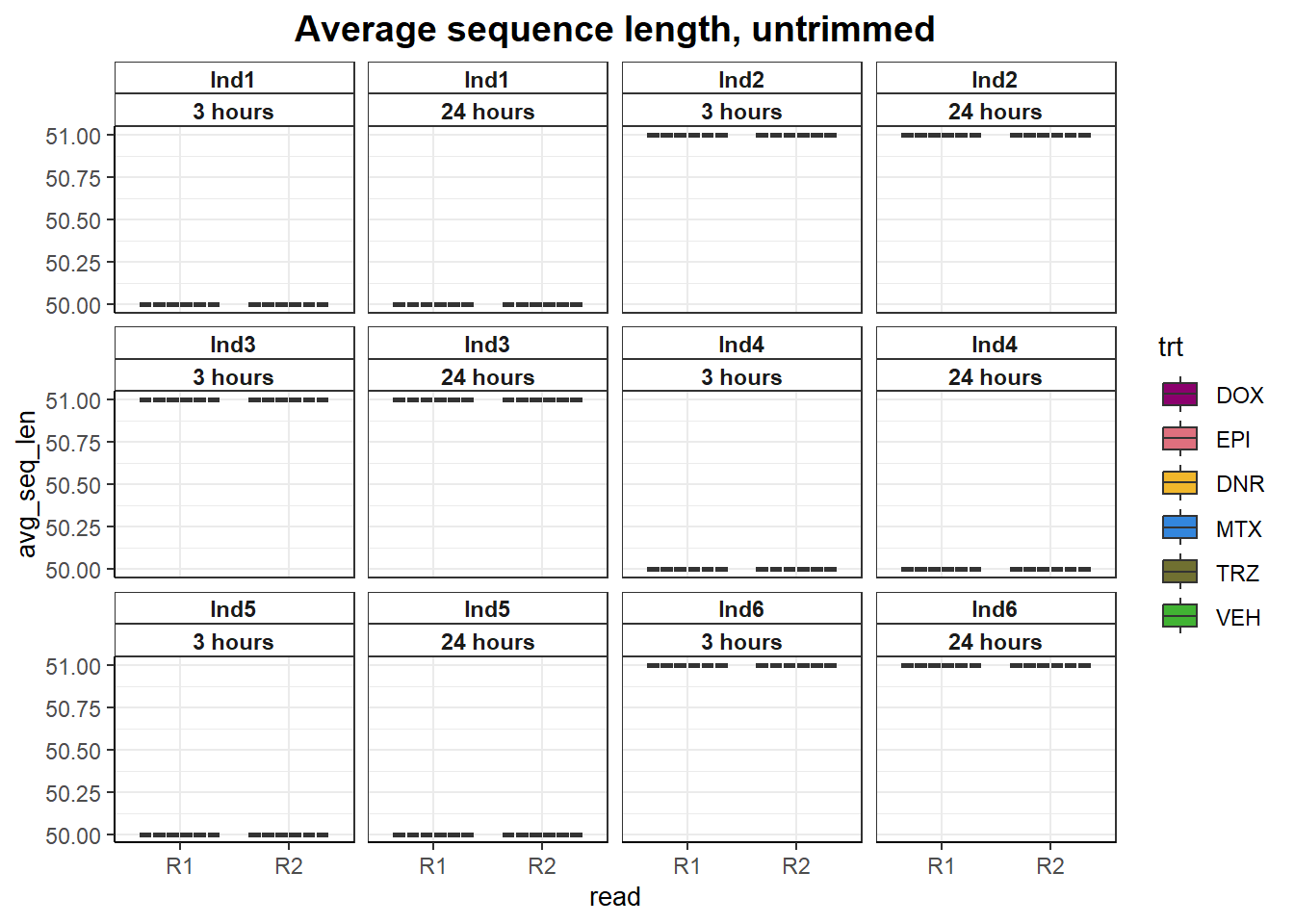
| Version | Author | Date |
|---|---|---|
| 3e9762b | reneeisnowhere | 2024-01-30 |
fastqc_full %>%
  filter(trimmed=="yes") %>%
   mutate(avg_sequence_length=as.numeric(avg_sequence_length)) %>%
  ggplot(., aes(x=read, y= avg_seq_len))+
  geom_boxplot(aes(col= trt))+
  facet_wrap(ind~time)+
  scale_fill_manual(values=drug_pal)+
  scale_color_manual(values = drug_pal)+
  theme_bw()+
  ggtitle("Average sequence length, trimmed")+
      # ylab(ylab)+
      # xlab("")+
      theme(strip.background = element_rect(fill = "white",linetype=1, linewidth = 0.5),
          plot.title = element_text(size=14,hjust = 0.5,face="bold"),
          axis.title = element_text(size = 10, color = "black"),
          axis.ticks = element_line(linewidth = 0.5),
          axis.line = element_line(linewidth = 0.5),
          # axis.text.x = element_blank(),
          strip.text.x = element_text(margin = margin(2,0,2,0, "pt"),face = "bold"))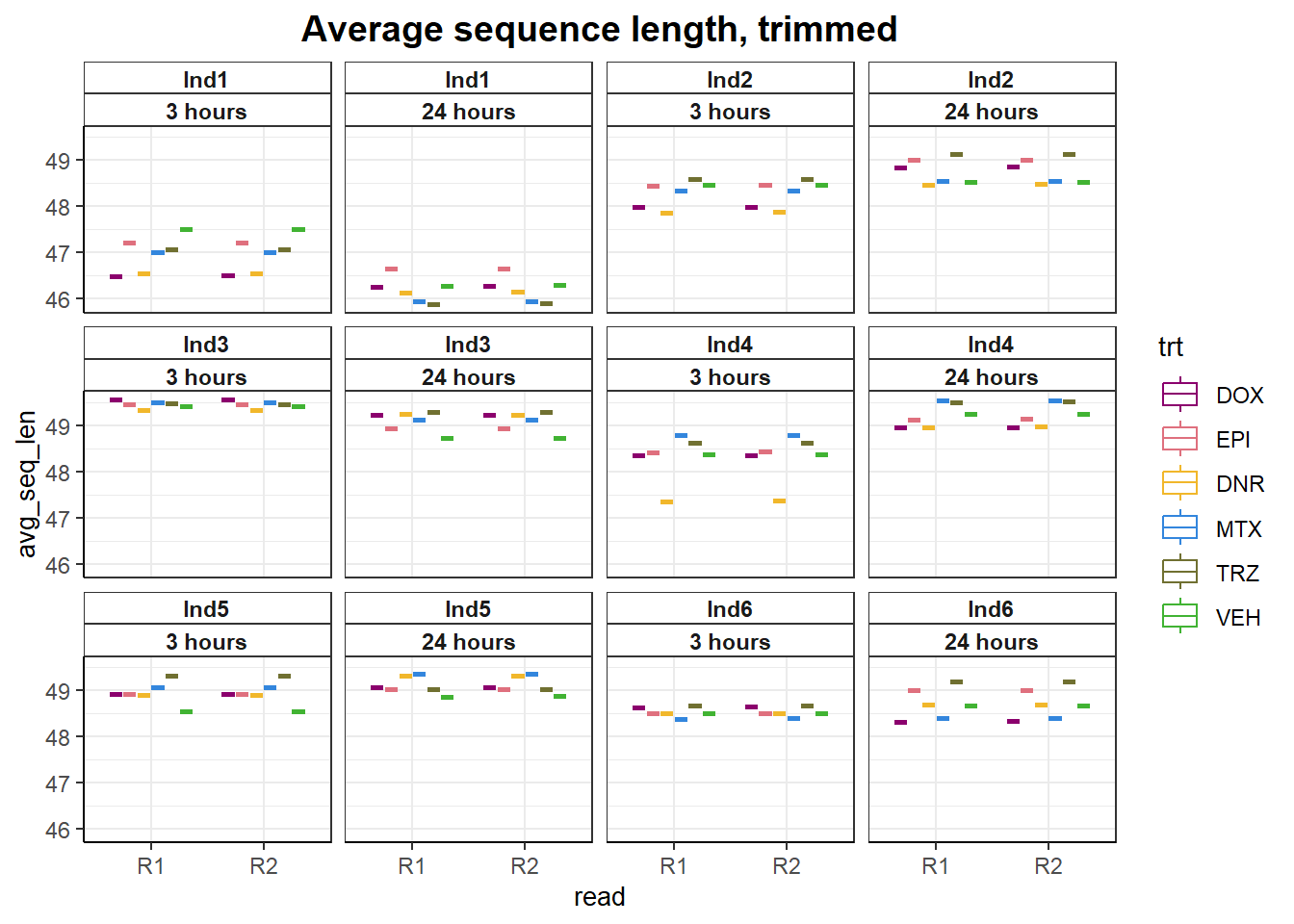
| Version | Author | Date |
|---|---|---|
| 3e9762b | reneeisnowhere | 2024-01-30 |
fastqc_full %>%

  filter(trimmed=="no") %>%
  group_by(trt) %>%
  # mutate(avg_sequence_length=as.numeric(avg_sequence_length)) %>%
  ggplot(., aes(x=read, y= percent_dup))+
  geom_col(position= "dodge",aes(fill= trt))+
  geom_text(aes(group=trt,label = sprintf("%.1f",percent_dup)),
            position=position_dodge(width =.95),angle= 90,vjust=.02, hjust=.7 )+
  facet_wrap(ind~time)+
  scale_fill_manual(values=drug_pal)+
  theme_bw()+
  # ylim(0,55)+
  ggtitle("Percent duplicated, untrimmed")+
      # ylab(ylab)+
      # xlab("")+
      theme(strip.background = element_rect(fill = "white",linetype=1, linewidth = 0.5),
          plot.title = element_text(size=14,hjust = 0.5,face="bold"),
          axis.title = element_text(size = 10, color = "black"),
          axis.ticks = element_line(linewidth = 0.5),
          axis.line = element_line(linewidth = 0.5),
          # axis.text.x = element_blank(),
          strip.text.x = element_text(margin = margin(2,0,2,0, "pt"),face = "bold"))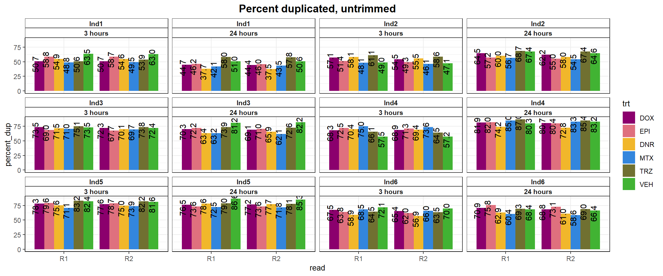
| Version | Author | Date |
|---|---|---|
| 3e9762b | reneeisnowhere | 2024-01-30 |
fastqc_full %>%
  filter(trimmed=="yes") %>%
   group_by(trt) %>%
  # mutate(avg_sequence_length=as.numeric(avg_sequence_length)) %>%
  ggplot(., aes(x=read, y= percent_dup))+
  geom_col(position= "dodge",aes(fill= trt))+
  geom_text(aes(group=trt,label = sprintf("%.1f",percent_dup)),
            position=position_dodge(width =.95),angle= 90,vjust=.02, hjust=.7 )+
  facet_wrap(ind~time)+
  scale_fill_manual(values=drug_pal)+
  theme_bw()+
      theme(strip.background = element_rect(fill = "white",linetype=1, linewidth = 0.5),
          plot.title = element_text(size=14,hjust = 0.5,face="bold"),
          axis.title = element_text(size = 10, color = "black"),
          axis.ticks = element_line(linewidth = 0.5),
          axis.line = element_line(linewidth = 0.5),
          # axis.text.x = element_blank(),
          strip.text.x = element_text(margin = margin(2,0,2,0, "pt"),face = "bold"))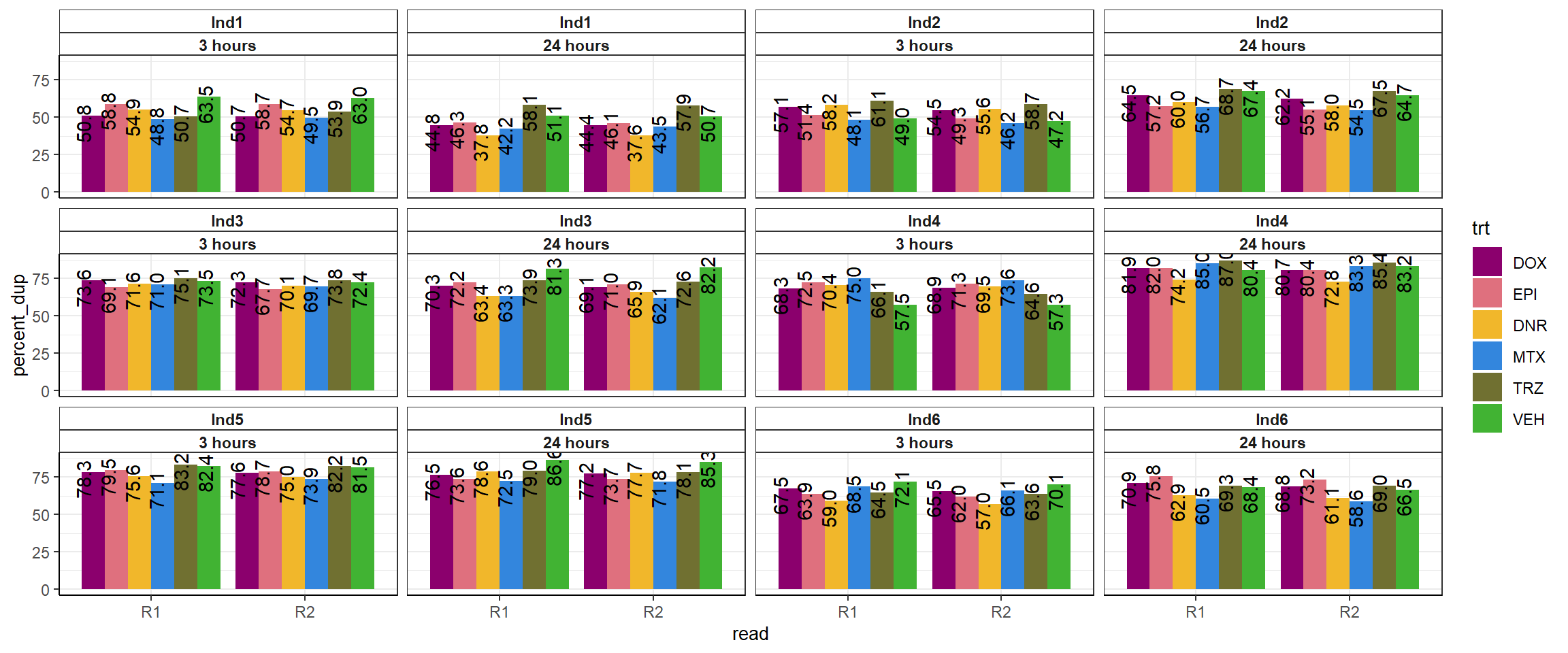
| Version | Author | Date |
|---|---|---|
| 3e9762b | reneeisnowhere | 2024-01-30 |
Trimmed sequence lengths
###omitted the first288 lines (this was a duplicate of the first multiqc run... changed files to iterate over in the furture)


trimmed_seq_length <- read.csv("data/trimmed_seq_length.csv", row.names = 1, col.names = 0:25)
# save <-
trimmed_seq_length <- trimmed_seq_length %>%
  rename( "0bp"=X0,"2bp"=X1,"4bp"=X2,"6bp"=X3,"8bp"=X4,"10bp"=X5,"12bp"=X6, "14bp"=X7, "16bp"=X8, "18bp"=X9, "20bp"=X10, "22bp"=X11, "24bp"=X12, "26bp"=X13, "28bp"=X14, "30bp"=X15, "32bp"=X16, "34bp"=X17, "36bp"=X18, "38bp"=X19, "40bp"=X20, "42bp"=X21, "44bp"=X22, "46bp"=X23, "48bp"=X24, "50bp"=X25)# %>%
  # column_to_rownames("samples") %>% write.csv(.,"data/trimmed_seq_length.csv")
#   t() %>%
# as.numeric()
# trimmed_seq_length %>%
#   rownames_to_column("samples") %>%
#   pivot_longer(., col=!samples, names_to = "frag_length", values_to = "counts")
#
#
#
# pivot_longer(everything(), names_to = "lelsngth", values_to ="counts")
# str(save)
aln_results <- read.csv("data/aln_run1_results.txt", row.names = 1)
aln_results %>%
mutate(treatment=factor(treatment, levels = c("DOX","EPI","DNR","MTX", "TRZ", "VEH"))) %>%
mutate(time=factor(time, levels = c("3","24"),labels=c("3 hours", "24 hours"))) %>%
mutate(indv=factor(indv, levels =c ("1","2","3","4","5","6"))) %>%
ggplot(., aes(x =time, y= reads), group= time)+
geom_boxplot(position = "dodge",aes(fill=treatment))+
geom_point(aes(col=indv))+
facet_wrap(~treatment)+
theme_bw()+
ggtitle("number of read-pairs")+
scale_fill_manual(values=drug_pal) +
scale_color_brewer(palette ="Dark2")+
theme(strip.background = element_rect(fill = "white",linetype=1, linewidth = 0.5),
plot.title = element_text(size=14,hjust = 0.5,face="bold"),
axis.title = element_text(size = 10, color = "black"),
axis.ticks = element_line(linewidth = 0.5),
axis.line = element_line(linewidth = 0.5),
# axis.text.x = element_blank(),
strip.text.x = element_text(margin = margin(2,0,2,0, "pt"),face = "bold"))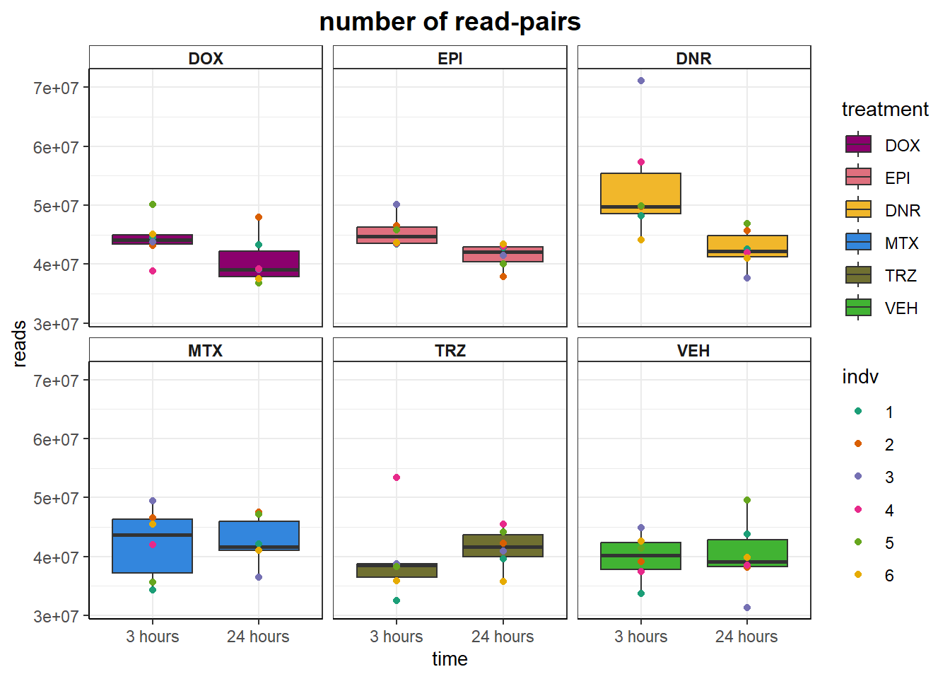
aln_results %>%
  mutate(treatment=factor(treatment, levels = c("DOX","EPI","DNR","MTX", "TRZ", "VEH"))) %>%
  mutate(time=factor(time, levels = c("3","24"),labels=c("3 hours", "24 hours"))) %>%
  mutate(indv=factor(indv, levels =c ("1","2","3","4","5","6"))) %>%

  ggplot(., aes(x =time, y= aln_overall), group= time)+
  geom_col(position= "dodge",aes(fill= treatment))+
  geom_text(aes(group=treatment,label = sprintf("%.1f",aln_overall*100)),
            position=position_dodge(width =.93),angle= 90,vjust=.1, hjust=.9 )+
  facet_wrap(~indv)+
  scale_fill_manual(values=drug_pal)+
  theme_bw()+
  ggtitle("Percent mapped reads")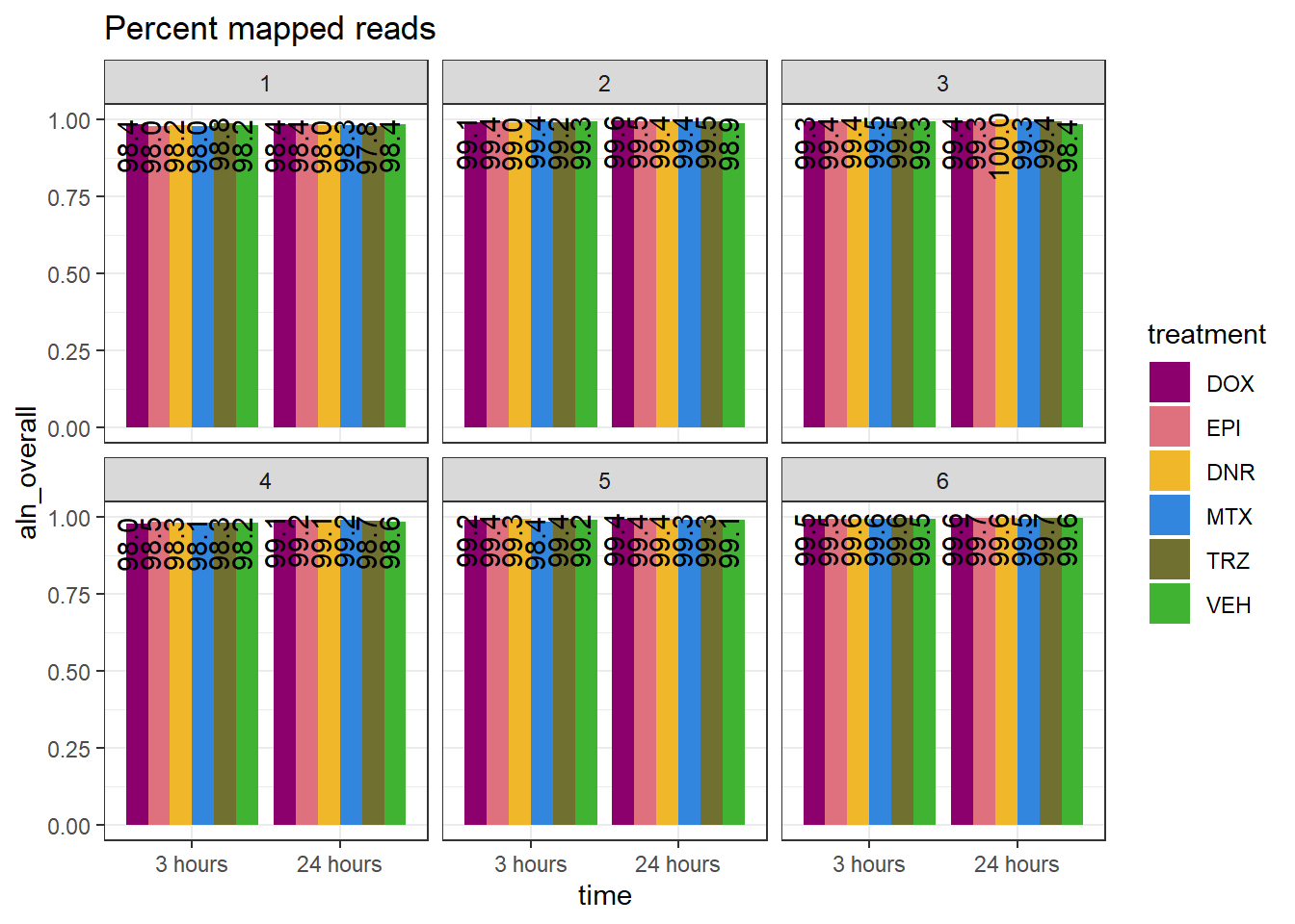
      theme(strip.background = element_rect(fill = "white",linetype=1, linewidth = 0.5),
          plot.title = element_text(size=14,hjust = 0.5,face="bold"),
          axis.title = element_text(size = 10, color = "black"),
          axis.ticks = element_line(linewidth = 0.5),
          axis.line = element_line(linewidth = 0.5),
          # axis.text.x = element_blank(),
          strip.text.x = element_text(margin = margin(2,0,2,0, "pt"),face = "bold"))
List of 6
$ axis.title :List of 11
..$ family : NULL
..$ face : NULL
..$ colour : chr "black"
..$ size : num 10
..$ hjust : NULL
..$ vjust : NULL
..$ angle : NULL
..$ lineheight : NULL
..$ margin : NULL
..$ debug : NULL
..$ inherit.blank: logi FALSE
..- attr(*, "class")= chr [1:2] "element_text" "element"
$ axis.ticks :List of 6
..$ colour : NULL
..$ linewidth : num 0.5
..$ linetype : NULL
..$ lineend : NULL
..$ arrow : logi FALSE
..$ inherit.blank: logi FALSE
..- attr(*, "class")= chr [1:2] "element_line" "element"
$ axis.line :List of 6
..$ colour : NULL
..$ linewidth : num 0.5
..$ linetype : NULL
..$ lineend : NULL
..$ arrow : logi FALSE
..$ inherit.blank: logi FALSE
..- attr(*, "class")= chr [1:2] "element_line" "element"
$ plot.title :List of 11
..$ family : NULL
..$ face : chr "bold"
..$ colour : NULL
..$ size : num 14
..$ hjust : num 0.5
..$ vjust : NULL
..$ angle : NULL
..$ lineheight : NULL
..$ margin : NULL
..$ debug : NULL
..$ inherit.blank: logi FALSE
..- attr(*, "class")= chr [1:2] "element_text" "element"
$ strip.background:List of 5
..$ fill : chr "white"
..$ colour : NULL
..$ linewidth : num 0.5
..$ linetype : num 1
..$ inherit.blank: logi FALSE
..- attr(*, "class")= chr [1:2] "element_rect" "element"
$ strip.text.x :List of 11
..$ family : NULL
..$ face : chr "bold"
..$ colour : NULL
..$ size : NULL
..$ hjust : NULL
..$ vjust : NULL
..$ angle : NULL
..$ lineheight : NULL
..$ margin : 'margin' num [1:4] 2points 0points 2points 0points
.. ..- attr(*, "unit")= int 8
..$ debug : NULL
..$ inherit.blank: logi FALSE
..- attr(*, "class")= chr [1:2] "element_text" "element"
- attr(*, "class")= chr [1:2] "theme" "gg"
- attr(*, "complete")= logi FALSE
- attr(*, "validate")= logi TRUEaln_results %>%
mutate(treatment=factor(treatment, levels = c("DOX","EPI","DNR","MTX", "TRZ", "VEH"))) %>%
mutate(time=factor(time, levels = c("3","24"),labels=c("3 hours", "24 hours"))) %>%
mutate(indv=factor(indv, levels =c ("1","2","3","4","5","6"))) %>%
# mutate(perc_aln_1_con= aln_1_con/reads * 100) %>%
ggplot(., aes(x =time, y= aln_1_con), group= time)+
geom_col(position= "dodge",aes(fill= treatment))+
# geom_text(aes(group=treatment,label = sprintf("%.1f",(aln_overall*100)),
# position=position_dodge(width =.95),angle= 90,vjust=.02, hjust=.7 ))+
facet_wrap(~indv)+
scale_fill_manual(values=drug_pal)+
theme_bw()+
ggtitle("number of concordantly aligned reads = 1")+
theme(strip.background = element_rect(fill = "white",linetype=1, linewidth = 0.5),
plot.title = element_text(size=14,hjust = 0.5,face="bold"),
axis.title = element_text(size = 10, color = "black"),
axis.ticks = element_line(linewidth = 0.5),
axis.line = element_line(linewidth = 0.5),
# axis.text.x = element_blank(),
strip.text.x = element_text(margin = margin(2,0,2,0, "pt"),face = "bold"))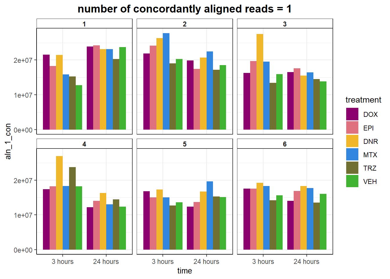
aln_results %>%
  mutate(treatment=factor(treatment, levels = c("DOX","EPI","DNR","MTX", "TRZ", "VEH"))) %>%
  mutate(time=factor(time, levels = c("3","24"),labels=c("3 hours", "24 hours"))) %>%
  mutate(indv=factor(indv, levels =c ("1","2","3","4","5","6"))) %>%
  mutate(perc_aln_1_con= aln_1_con/reads * 100) %>%

  ggplot(., aes(x =time, y= perc_aln_1_con), group= time)+
  geom_col(position= "dodge",aes(fill= treatment))+
  geom_text(aes(group=treatment,label = sprintf("%.1f",perc_aln_1_con)),
            position=position_dodge(width =.95),angle= 90,vjust=.02, hjust=.7 )+
  facet_wrap(~indv)+
  scale_fill_manual(values=drug_pal)+
  theme_bw()+
  ggtitle("Percent of concordantly aligned reads = 1")+
      theme(strip.background = element_rect(fill = "white",linetype=1, linewidth = 0.5),
          plot.title = element_text(size=14,hjust = 0.5,face="bold"),
          axis.title = element_text(size = 10, color = "black"),
          axis.ticks = element_line(linewidth = 0.5),
          axis.line = element_line(linewidth = 0.5),
          # axis.text.x = element_blank(),
          strip.text.x = element_text(margin = margin(2,0,2,0, "pt"),face = "bold"))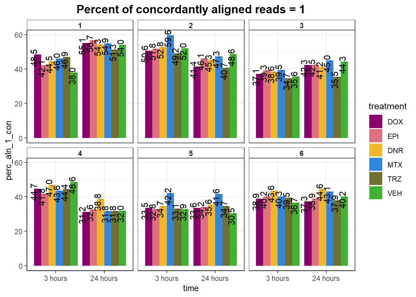
aln_results %>%
  mutate(treatment=factor(treatment, levels = c("DOX","EPI","DNR","MTX", "TRZ", "VEH"))) %>%
  mutate(time=factor(time, levels = c("3","24"),labels=c("3 hours", "24 hours"))) %>%
  mutate(indv=factor(indv, levels =c ("1","2","3","4","5","6"))) %>%
  mutate(perc_multimapped= aln_.1_con/reads * 100) %>%

  ggplot(., aes(x =time, y= perc_multimapped), group= time)+
  geom_col(position= "dodge",aes(fill= treatment))+
  geom_text(aes(group=treatment,label = sprintf("%.1f",perc_multimapped)),
            position=position_dodge(width =.93),angle= 90,vjust=.02, hjust=.7 )+
  facet_wrap(~indv)+
  scale_fill_manual(values=drug_pal)+
  theme_bw()+
  ggtitle("Percent of aligned reads > 1")+
      theme(strip.background = element_rect(fill = "white",linetype=1, linewidth = 0.5),
          plot.title = element_text(size=14,hjust = 0.5,face="bold"),
          axis.title = element_text(size = 10, color = "black"),
          axis.ticks = element_line(linewidth = 0.5),
          axis.line = element_line(linewidth = 0.5),
          # axis.text.x = element_blank(),
          strip.text.x = element_text(margin = margin(2,0,2,0, "pt"),face = "bold"))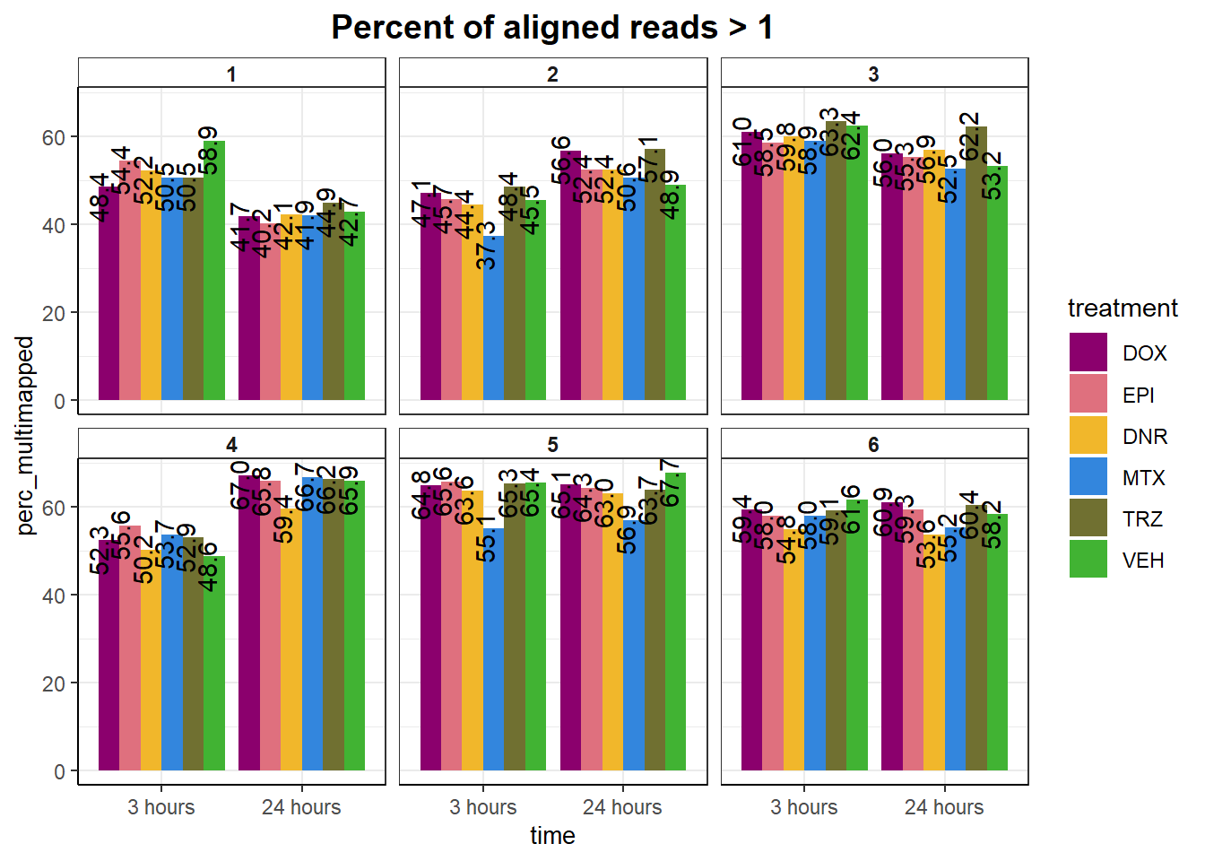
Peaks
Ind1_75DA24h_dedup_peaks <- read.csv("data/Ind1_75DA24h_dedup_peaks.csv", row.names = 1)

Ind4_79V24h_dedup_peaks <-  ##(misspelled)
  read.csv("data/Ind4_79B24h_dedup_peaks.csv", row.names = 1)
plot fragment length
Ind1_75DA24h_dedup_peaks %>%
  ggplot(., aes(x= length))+
  geom_density()+
  ggtitle("Ind1 DNR 24h")+
  xlim(0,10^3)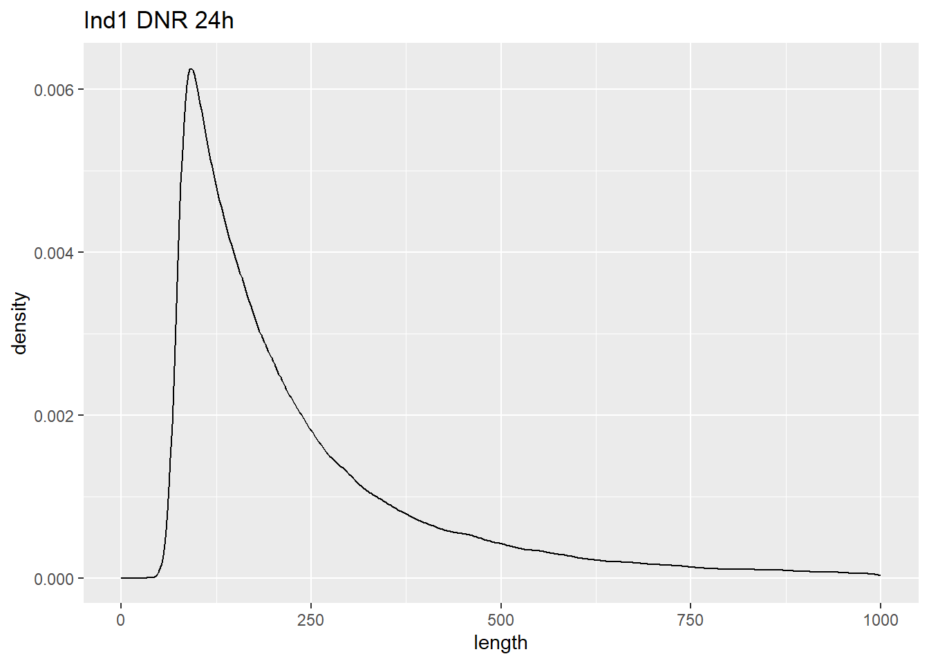
Ind4_79V24h_dedup_peaks %>%
  ggplot(., aes(x= length))+
  geom_density()+
  ggtitle("Ind4 VEH 24h")+
  xlim(0,10^3)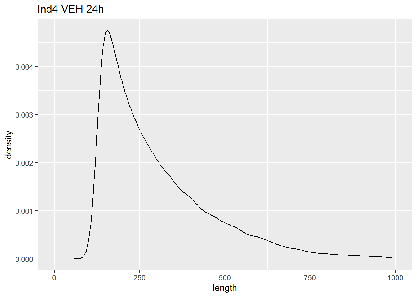
)
sessionInfo()R version 4.3.1 (2023-06-16 ucrt)
Platform: x86_64-w64-mingw32/x64 (64-bit)
Running under: Windows 10 x64 (build 19045)
Matrix products: default
locale:
[1] LC_COLLATE=English_United States.utf8
[2] LC_CTYPE=English_United States.utf8
[3] LC_MONETARY=English_United States.utf8
[4] LC_NUMERIC=C
[5] LC_TIME=English_United States.utf8
time zone: America/Chicago
tzcode source: internal
attached base packages:
[1] stats graphics grDevices utils datasets methods base
other attached packages:
[1] RColorBrewer_1.1-3 kableExtra_1.3.4 lubridate_1.9.3 forcats_1.0.0
[5] stringr_1.5.0 dplyr_1.1.3 purrr_1.0.2 readr_2.1.4
[9] tidyr_1.3.0 tibble_3.2.1 ggplot2_3.4.4 tidyverse_2.0.0
[13] workflowr_1.7.1
loaded via a namespace (and not attached):
[1] gtable_0.3.4 xfun_0.41 bslib_0.6.1 processx_3.8.2
[5] callr_3.7.3 tzdb_0.4.0 vctrs_0.6.4 tools_4.3.1
[9] ps_1.7.5 generics_0.1.3 parallel_4.3.1 fansi_1.0.5
[13] highr_0.10 pkgconfig_2.0.3 webshot_0.5.5 lifecycle_1.0.4
[17] farver_2.1.1 compiler_4.3.1 git2r_0.32.0 munsell_0.5.0
[21] getPass_0.2-2 httpuv_1.6.12 htmltools_0.5.7 sass_0.4.7
[25] yaml_2.3.7 crayon_1.5.2 later_1.3.1 pillar_1.9.0
[29] jquerylib_0.1.4 whisker_0.4.1 cachem_1.0.8 tidyselect_1.2.0
[33] rvest_1.0.3 digest_0.6.33 stringi_1.7.12 labeling_0.4.3
[37] rprojroot_2.0.4 fastmap_1.1.1 grid_4.3.1 colorspace_2.1-0
[41] cli_3.6.1 magrittr_2.0.3 utf8_1.2.4 withr_3.0.0
[45] scales_1.3.0 promises_1.2.1 bit64_4.0.5 timechange_0.2.0
[49] rmarkdown_2.25 httr_1.4.7 bit_4.0.5 hms_1.1.3
[53] evaluate_0.23 knitr_1.45 viridisLite_0.4.2 rlang_1.1.2
[57] Rcpp_1.0.11 glue_1.6.2 xml2_1.3.5 svglite_2.1.2
[61] rstudioapi_0.15.0 vroom_1.6.5 jsonlite_1.8.7 R6_2.5.1
[65] systemfonts_1.0.5 fs_1.6.3