Last updated: 2021-09-13

Checks: 6 1

Knit directory: project_video_salience/

This reproducible R Markdown analysis was created with workflowr (version 1.6.2). The Checks tab describes the reproducibility checks that were applied when the results were created. The Past versions tab lists the development history.

R Markdown file: up-to-date

Great! Since the R Markdown file has been committed to the Git repository, you know the exact version of the code that produced these results.

Environment: empty

Great job! The global environment was empty. Objects defined in the global environment can affect the analysis in your R Markdown file in unknown ways. For reproduciblity it’s best to always run the code in an empty environment.

Seed: set.seed(20210113)

The command set.seed(20210113) was run prior to running the code in the R Markdown file. Setting a seed ensures that any results that rely on randomness, e.g. subsampling or permutations, are reproducible.

Session information: recorded

Great job! Recording the operating system, R version, and package versions is critical for reproducibility.

Cache: detected

The following chunks had caches available:

age_groups
data_preparation
exclude_missing_deviating_cases
func_p_correction
grand_average_PD
group_differences
load_preprocessed_data
match_groups
merge_motion_and_perceptual_salience_data
merge_saccade_fixation_data
missings_in_clinical_variables
PCA_pupillary_response
polynomial_fit_comparison
power_analysis
progression_of_key_variables
results_motion_salience
results_physical_salience
results_social_attention_with_pupillarycomponents
results_social_attention_with_pupillaryresponse
sample descriptive statistics
scenes_duration
session-info-chunk-inserted-by-workflowr
workspace_cleanup

To ensure reproducibility of the results, delete the cache directory data_analysis_salience_cache and re-run the analysis. To have workflowr automatically delete the cache directory prior to building the file, set delete_cache = TRUE when running wflow_build() or wflow_publish().

File paths: relative

Great job! Using relative paths to the files within your workflowr project makes it easier to run your code on other machines.

Repository version: 4485527

Great! You are using Git for version control. Tracking code development and connecting the code version to the results is critical for reproducibility.

The results in this page were generated with repository version 4485527. See the Past versions tab to see a history of the changes made to the R Markdown and HTML files.

Note that you need to be careful to ensure that all relevant files for the analysis have been committed to Git prior to generating the results (you can use wflow_publish or wflow_git_commit). workflowr only checks the R Markdown file, but you know if there are other scripts or data files that it depends on. Below is the status of the Git repository when the results were generated:


Ignored files:
    Ignored:    .Rhistory
    Ignored:    .Rproj.user/
    Ignored:    analysis/data_analysis_salience_cache/

Untracked files:
    Untracked:  .PowerFolder/
    Untracked:  analysis/Results in unmatched sample.docx
    Untracked:  code/OLD/
    Untracked:  code/analysis_salience_130121.R
    Untracked:  code/analysis_salience_150421.R
    Untracked:  code/mean_salience_per_video.R
    Untracked:  code/preprocessing1_matching_gaze_and_salience_data.R
    Untracked:  code/preprocessing2_matching_gaze_and_motionsalience_data.R
    Untracked:  code/preprocessing3_datareduction_adding_additional_data.R
    Untracked:  code/python_code_salience_extraction/
    Untracked:  code/sesnory_subgroup_analysis.R
    Untracked:  data/merged_data/
    Untracked:  data/video_stimuli_scenes.csv
    Untracked:  desktop.ini
    Untracked:  manuscript/
    Untracked:  output/gaze_animate_sample.mp4
    Untracked:  output/gaze_animate_sample_dollhouse_scene5.mp4
    Untracked:  output/motion_salience/
    Untracked:  output/motion_salience_video_pingudoctors_scene0.avi
    Untracked:  output/salience_video_artist.avi
    Untracked:  output/stimuli_pics/
    Untracked:  output/stimuli_salience/
    Untracked:  output/stimuli_scene/
    Untracked:  project_init_workflow.R

Unstaged changes:
    Modified:   code/README.md
    Modified:   data/README.md

Note that any generated files, e.g. HTML, png, CSS, etc., are not included in this status report because it is ok for generated content to have uncommitted changes.

These are the previous versions of the repository in which changes were made to the R Markdown (analysis/data_analysis_salience.Rmd) and HTML (docs/data_analysis_salience.html) files. If you’ve configured a remote Git repository (see ?wflow_git_remote), click on the hyperlinks in the table below to view the files as they were in that past version.

File	Version	Author	Date	Message
Rmd	4485527	nicobast	2021-09-13	Publish the initial files for myproject

data merging

fixation data and saccade data was previously preprocessed as separate files. These are now merged by saccade before a fixation. motion salience data is also merged with perceptual salience data

sample definition

also described in flow chart (see figure folder)

exclude cases (sample flow chart)

excluded. Missing demographic data, deviating IQ, ADOS comparative severity below clinical cutoff

## EXCLUDE CASES ####
      
      print('sample with available data / before exclusion:')

[1] "sample with available data / before exclusion:"

      nrow(df_agg)

[1] 543

      with(df_agg,table(t1_diagnosis))

t1_diagnosis
    ASD Control 
    315     228

  #DEMOGRAPHIC OUTLIER:
      #table(is.na(df_agg$t1_ageyrs)) #no missings
      #table(is.na(df_agg$t1_sex)) # no missings
      
      by(is.na(df_agg$t1_piq),df_agg$t1_diagnosis,table) #missing IQ data

df_agg$t1_diagnosis: ASD

FALSE  TRUE 
  310     5 
------------------------------------------------------------ 
df_agg$t1_diagnosis: Control

FALSE  TRUE 
  226     2

      by(df_agg$t1_piq<=60 | df_agg$t1_piq>=140,df_agg$t1_diagnosis,table) #IQ outlier

df_agg$t1_diagnosis: ASD

FALSE  TRUE 
  294    16 
------------------------------------------------------------ 
df_agg$t1_diagnosis: Control

FALSE  TRUE 
  219     7

      by(df_agg$SR==60,df_agg$t1_diagnosis,table) #sampling rate = 60hz

df_agg$t1_diagnosis: ASD

FALSE  TRUE 
  311     4 
------------------------------------------------------------ 
df_agg$t1_diagnosis: Control

FALSE  TRUE 
  224     4

      ### --> n=544
      df_agg<-df_agg[df_agg$t1_piq>60 & df_agg$t1_piq<140,] #n=23
      df_agg<-df_agg[!is.na(df_agg$t1_piq),] #n=7
      df_agg<-df_agg[df_agg$SR!=60,] #n=8
      
          
  ###--> STUDY SAMPLE
      #with(df_agg[df_agg$t1_css_total_all>3 | df_agg$t1_diagnosis=='Control',],table(t1_sensory_subgroups,t1_diagnosis))
      
      table(df_agg$t1_diagnosis == 'Control' | (!is.na(df_agg$t1_css_total_all) & df_agg$t1_css_total_all>3))


FALSE  TRUE 
   99   406

      df_sample<-df_agg[df_agg$t1_diagnosis == 'Control' | (!is.na(df_agg$t1_css_total_all) & df_agg$t1_css_total_all>3),] 
          with(df_sample,table(t1_diagnosis))

t1_diagnosis
    ASD Control 
    191     215

      #n=101
      #n=99 excluded
      #df_sample<-df_agg
      
      nrow(df_sample)

[1] 406

match groups

match groups based on initial group differences

            
             ASD Control
  adolescent  84      82
  adult       59      80
  child       48      53


    Welch Two Sample t-test

data:  t1_ageyrs by t1_diagnosis
t = -1.8108, df = 402.94, p-value = 0.07091
alternative hypothesis: true difference in means is not equal to 0
95 percent confidence interval:
 -2.15579668  0.08850771
sample estimates:
    mean in group ASD mean in group Control 
             15.94244              16.97608


    Welch Two Sample t-test

data:  t1_piq by t1_diagnosis
t = -4.3791, df = 382.03, p-value = 1.541e-05
alternative hypothesis: true difference in means is not equal to 0
95 percent confidence interval:
 -11.098979  -4.220616
sample estimates:
    mean in group ASD mean in group Control 
             100.0422              107.7020


    Pearson's Chi-squared test with Yates' continuity correction

data:  t1_sex and t1_diagnosis
X-squared = 1.6829, df = 1, p-value = 0.1945


    Welch Two Sample t-test

data:  Accuracy by t1_diagnosis
t = 5.1002, df = 295.37, p-value = 6.078e-07
alternative hypothesis: true difference in means is not equal to 0
95 percent confidence interval:
 0.2378880 0.5368347
sample estimates:
    mean in group ASD mean in group Control 
           0.07190785           -0.31545349


    Welch Two Sample t-test

data:  Precision by t1_diagnosis
t = 1.0249, df = 388.4, p-value = 0.3061
alternative hypothesis: true difference in means is not equal to 0
95 percent confidence interval:
 -0.07309426  0.23227557
sample estimates:
    mean in group ASD mean in group Control 
           -0.1031796            -0.1827702

### MATCHING sample by age, iq  ####  
      #sample size (n=406, --> matching process: ASD: n=75, TD: n=52)
      nrow(df_sample)

[1] 406

      with(df_sample,table(t1_diagnosis))

t1_diagnosis
    ASD Control 
    191     215

      #balancing based on age categories
      df_cov<-df_sample[,c('id','t1_ageyrs','t1_sex','t1_piq','t1_diagnosis','Accuracy','Precision')]
      groupBoo<-with(df_cov,ifelse(t1_diagnosis=='ASD',1,0))
      df_cov<-data.frame(df_cov,groupBoo)
      df_cov$piq<-round(df_cov$t1_piq) #round
      df_cov$age<-floor(df_cov$t1_ageyrs)
      
      #ALL - matching
      set.seed(100)
      all.match<-matchit(groupBoo~age+piq+Accuracy,
                         data=df_cov,
                         method='nearest',discard='both', 
                         replace=F,caliper=0.4)
      
      all.match


Call: 
matchit(formula = groupBoo ~ age + piq + Accuracy, data = df_cov, 
    method = "nearest", discard = "both", replace = F, caliper = 0.4)

Sample sizes:
          Control Treated
All           215     191
Matched       164     164
Unmatched      47      13
Discarded       4      14

      #remove cases in unaggregated data frame
      all.match<-match.data(all.match)
      df_sample<-df_sample[df_sample$id %in% all.match$id,]
      
      df_fix<-df_fix[df_fix$id %in% all.match$id,]
      df_sac<-df_sac[df_sac$id %in% all.match$id,]
      df<-df[df$id %in% all.match$id,]

additional information

define age groups

no differences occured between age groups on key demographic variables

            
             ASD Control
  adolescent  73      63
  adult       53      55
  child       38      46


Call:
lm(formula = t1_ageyrs ~ t1_diagnosis * age_group)

Residuals:
    Min      1Q  Median      3Q     Max 
-5.3943 -1.8227  0.0485  1.4692  7.4550 

Coefficients:
                                   Estimate Std. Error t value Pr(>|t|)    
(Intercept)                         14.7828     0.2895  51.058   <2e-16 ***
t1_diagnosisControl                  0.7252     0.4254   1.705   0.0892 .  
age_groupadult                       8.1404     0.4464  18.235   <2e-16 ***
age_groupchild                      -5.1392     0.4948 -10.386   <2e-16 ***
t1_diagnosisControl:age_groupadult  -0.1280     0.6385  -0.201   0.8412    
t1_diagnosisControl:age_groupchild  -0.7717     0.6892  -1.120   0.2637    
---
Signif. codes:  0 '***' 0.001 '**' 0.01 '*' 0.05 '.' 0.1 ' ' 1

Residual standard error: 2.474 on 322 degrees of freedom
Multiple R-squared:  0.8228,    Adjusted R-squared:   0.82 
F-statistic:   299 on 5 and 322 DF,  p-value: < 2.2e-16


Call:
lm(formula = t1_piq ~ t1_diagnosis * age_group)

Residuals:
    Min      1Q  Median      3Q     Max 
-40.399 -11.332   1.027  12.476  36.687 

Coefficients:
                                   Estimate Std. Error t value Pr(>|t|)    
(Intercept)                        100.3104     2.0427  49.106   <2e-16 ***
t1_diagnosisControl                  2.6660     3.0013   0.888   0.3751    
age_groupadult                       1.0885     3.1496   0.346   0.7299    
age_groupchild                       6.4183     3.4912   1.838   0.0669 .  
t1_diagnosisControl:age_groupadult   0.9056     4.5048   0.201   0.8408    
t1_diagnosisControl:age_groupchild  -0.9157     4.8627  -0.188   0.8507    
---
Signif. codes:  0 '***' 0.001 '**' 0.01 '*' 0.05 '.' 0.1 ' ' 1

Residual standard error: 17.45 on 322 degrees of freedom
Multiple R-squared:  0.02621,   Adjusted R-squared:  0.01109 
F-statistic: 1.733 on 5 and 322 DF,  p-value: 0.1265


Call:
glm(formula = as.factor(t1_sex) ~ t1_diagnosis * age_group, family = binomial)

Deviance Residuals: 
    Min       1Q   Median       3Q      Max  
-1.8174  -1.4110   0.8157   0.8740   0.9606  

Coefficients:
                                   Estimate Std. Error z value Pr(>|z|)    
(Intercept)                          1.4385     0.2973   4.839 1.31e-06 ***
t1_diagnosisControl                 -0.6730     0.4020  -1.674   0.0941 .  
age_groupadult                      -0.5089     0.4259  -1.195   0.2321    
age_groupchild                      -0.7846     0.4531  -1.732   0.0834 .  
t1_diagnosisControl:age_groupadult   0.6344     0.5855   1.084   0.2785    
t1_diagnosisControl:age_groupchild   0.5532     0.6098   0.907   0.3643    
---
Signif. codes:  0 '***' 0.001 '**' 0.01 '*' 0.05 '.' 0.1 ' ' 1

(Dispersion parameter for binomial family taken to be 1)

    Null deviance: 394.80  on 327  degrees of freedom
Residual deviance: 389.01  on 322  degrees of freedom
AIC: 401.01

Number of Fisher Scoring iterations: 4


Call:
lm(formula = Accuracy ~ t1_diagnosis * age_group)

Residuals:
    Min      1Q  Median      3Q     Max 
-1.3152 -0.4180 -0.1557  0.2599  2.4077 

Coefficients:
                                   Estimate Std. Error t value Pr(>|t|)  
(Intercept)                        -0.12669    0.07003  -1.809   0.0714 .
t1_diagnosisControl                -0.11535    0.10290  -1.121   0.2631  
age_groupadult                     -0.04448    0.10798  -0.412   0.6807  
age_groupchild                     -0.15934    0.11969  -1.331   0.1840  
t1_diagnosisControl:age_groupadult  0.03968    0.15444   0.257   0.7974  
t1_diagnosisControl:age_groupchild  0.13854    0.16671   0.831   0.4066  
---
Signif. codes:  0 '***' 0.001 '**' 0.01 '*' 0.05 '.' 0.1 ' ' 1

Residual standard error: 0.5984 on 322 degrees of freedom
Multiple R-squared:  0.009191,  Adjusted R-squared:  -0.006194 
F-statistic: 0.5974 on 5 and 322 DF,  p-value: 0.702


Call:
lm(formula = Accuracy ~ t1_diagnosis * age_group)

Residuals:
    Min      1Q  Median      3Q     Max 
-1.3152 -0.4180 -0.1557  0.2599  2.4077 

Coefficients:
                                   Estimate Std. Error t value Pr(>|t|)  
(Intercept)                        -0.12669    0.07003  -1.809   0.0714 .
t1_diagnosisControl                -0.11535    0.10290  -1.121   0.2631  
age_groupadult                     -0.04448    0.10798  -0.412   0.6807  
age_groupchild                     -0.15934    0.11969  -1.331   0.1840  
t1_diagnosisControl:age_groupadult  0.03968    0.15444   0.257   0.7974  
t1_diagnosisControl:age_groupchild  0.13854    0.16671   0.831   0.4066  
---
Signif. codes:  0 '***' 0.001 '**' 0.01 '*' 0.05 '.' 0.1 ' ' 1

Residual standard error: 0.5984 on 322 degrees of freedom
Multiple R-squared:  0.009191,  Adjusted R-squared:  -0.006194 
F-statistic: 0.5974 on 5 and 322 DF,  p-value: 0.702

missings in clinical variables

[1] "missing ADHD inattention data:"

     TRUE 
0.1707317

[1] "missing ADHD hyperactivity data:"

     TRUE 
0.1707317

[1] "missing Beck anxiety data"

     TRUE 
0.2317073

[1] "missing Beck depression data"

     TRUE 
0.2103659

grand average PD

variable is used in CFA

data selection

define scene duration

  ##DEFINE TIME SPAN ####
  df_scenes$vid_social<-ifelse(df_scenes$vid.id %in% c('50faces.mov','dollhouse.m4v','musicbooth.mov'),T,F)
  
  hist(diff(df_scenes$scene_time_onset)[diff(df_scenes$scene_time_onset)>0 & diff(df_scenes$scene_time_onset)<20000],30,
       xlab = 'time (ms)',main = 'duration of individual scenes',col='grey')
  abline(v=5000,lty=2)

      #create figure scene duration
      tiff(file="manuscript/figures/figure_sceneduration.tiff", # create a file in tiff format in current working directory
      width=6, height=4, units="in", res=300, compression='lzw') #define size and resolution of the resulting figure
      
      hist(diff(df_scenes$scene_time_onset)[diff(df_scenes$scene_time_onset)>0 & diff(df_scenes$scene_time_onset)<20000],30,
           xlab = 'time (ms)',col='grey',main='')
      abline(v=5000,lty=2)
      
      dev.off() #close operation and save file

png 
  2

      #human scenes
      hist(diff(df_scenes$scene_time_onset[df_scenes$vid_social==T])[diff(df_scenes$scene_time_onset[df_scenes$vid_social==T])>0 & diff(df_scenes$scene_time_onset[df_scenes$vid_social==T])<20000],30,
           xlab = 'time (ms)',main = 'duration of individual scenes (AOI scenes)',col='grey')
      abline(v=5000,col="red")

      #non human scenes
      hist(diff(df_scenes$scene_time_onset[df_scenes$vid_social==F])[diff(df_scenes$scene_time_onset[df_scenes$vid_social==F])>0 & diff(df_scenes$scene_time_onset[df_scenes$vid_social==F])<20000],30,
           xlab = 'time (ms)',main = 'duration of individual scenes (non AOI scenes)',col='grey')
      abline(v=5000,col="red")

  #-->most scenes are shorter than 6 seconds
  
  median(diff(df_scenes$scene_time_onset)[diff(df_scenes$scene_time_onset)>0])

[1] 2880

  sd(diff(df_scenes$scene_time_onset)[diff(df_scenes$scene_time_onset)>0])

[1] 3543.542

  #number of scenes:
  length(table(droplevels(interaction(df$vid_scene_nr,df$vid.id))))

[1] 85

    #human scenes
    length(table(droplevels(interaction(df$vid_scene_nr[df$vid.id %in% c('50faces.mov','dollhouse.m4v','musicbooth.mov')],df$vid.id[df$vid.id %in% c('50faces.mov','dollhouse.m4v','musicbooth.mov')]))))

[1] 36

    #scenes only presented in adolescents and adults
    length(table(droplevels(interaction(df$vid_scene_nr[df$vid.id %in% c('dollhouse.m4v','musicbooth.mov')],df$vid.id[df$vid.id %in% c('dollhouse.m4v','musicbooth.mov')]))))

[1] 21

prepare data

prepare data set

calcualte additional required variables. scaling of variables

extract pupillary components

png 
  2

results

define function p-correction

supporting analyses

polynomial fit comparison

Comparison of polynomial fits: pupillary response
model	parameters (n)	AIC	BIC	logLik	deviance	Chisq	df	p
first degree	15	173150.7	173287.7	-86560.33	173120.7	NA	NA	NA
second degree	16	173151.9	173298.0	-86559.94	173119.9	0.786	1	0.375
third degree	17	173149.0	173304.3	-86557.52	173115.0	4.838	1	0.028
fourth degree	18	173150.7	173315.1	-86557.37	173114.7	0.300	1	0.584

power analysis

sample descriptive statistics

Sample description
	ASD	TD	p-value
n	164	164	NA
age	16.22/5.63	16.54/6.04	0.626
gender (F/M)	42/122	53/111	0.223
non-verbal IQ	102.15/18.11	105.19/16.89	0.117
data quality - accuracy	-0.18/0.62	-0.25/0.57	0.278
data quality - precision	-0.12/0.8	-0.11/0.77	0.946
SRS total	97.29/29.63	27.59/19.83	0
ADHD inatt	4.38/3.16	1.26/2	0
anxiety (BAS)	15.11/11.45	7.2/6.05	0
depression (BDI)	14.78/12.35	5.9/5.82	0

progression of key variables

png 
  2

main analyses

sensory salience

                     2.5 % 97.5 %
vid_socialTRUE -0.29 -0.42  -0.15

            2.5 % 97.5 %
rpd_z -0.02 -0.04  -0.01

 contrast     estimate     SE  df asymp.LCL asymp.UCL
 FALSE - TRUE    0.266 0.0712 Inf     0.127     0.406

Results are averaged over the levels of: t1_diagnosis, t1_sex 
Note: contrasts are still on the scale scale 
Degrees-of-freedom method: asymptotic 
Confidence level used: 0.95

 vid_social rpd_z.trend      SE  df asymp.LCL asymp.UCL
 FALSE          -0.0360 0.00773 Inf   -0.0512  -0.02090
  TRUE          -0.0119 0.00937 Inf   -0.0303   0.00647

Results are averaged over the levels of: t1_diagnosis, t1_sex 
Degrees-of-freedom method: asymptotic 
Confidence level used: 0.95

Linear mixed model: physical salience
	Sum Sq	df1	df2	F	p	p_adj
group	1.488	1	263.953	1.704	0.193	0.579
pupillary response (PR)	17.759	1	56869.342	20.346	0.000	0.000
video category (VC)	13.128	1	79.824	15.040	0.000	0.000
time^1	8.803	1	68233.615	10.085	0.001	0.003
time^2	6.456	1	68247.752	7.396	0.007	0.021
time^3	4.577	1	68247.374	5.243	0.022	0.066
sex	0.000	1	241.875	0.000	0.985	1.000
age	0.934	1	270.110	1.070	0.302	0.906
perceptual IQ	1.575	1	266.350	1.804	0.180	0.540
ADHD inattention	1.838	1	272.232	2.105	0.148	0.444
anxiety	0.382	1	209.388	0.438	0.509	1.000
depression	0.071	1	223.502	0.082	0.775	1.000
accuracy	1.743	1	303.422	1.997	0.159	0.477
precision	0.082	1	369.914	0.093	0.760	1.000
center deviation	781.640	1	61947.894	895.506	0.000	0.000
group x PR	2.884	1	59515.863	3.304	0.069	0.207
group x VC	1.723	1	55964.028	1.974	0.160	0.480
PR x VC	6.212	1	31514.370	7.117	0.008	0.024
group x time^1	1.055	1	68183.309	1.208	0.272	0.816
group x time^2	0.819	1	68193.552	0.938	0.333	0.999
group x time^3	0.630	1	68197.508	0.722	0.396	1.000
PR x time^1	0.218	1	68201.553	0.250	0.617	1.000
PR x time^2	0.010	1	68221.075	0.011	0.916	1.000
PR x time^3	0.014	1	68226.630	0.016	0.899	1.000
VC x time^1	0.443	1	68228.689	0.507	0.476	1.000
VC x time^2	1.106	1	68243.382	1.267	0.260	0.780
VC x time^3	0.958	1	68246.420	1.097	0.295	0.885
group x PR x VC	0.048	1	32697.898	0.055	0.814	1.000
group x PR x time^1	0.594	1	68195.824	0.680	0.410	1.000
group x PR x time^2	0.193	1	68217.200	0.221	0.638	1.000
group x PR x time^3	0.027	1	68223.447	0.030	0.862	1.000
group x VC x time^1	0.235	1	68193.931	0.269	0.604	1.000
group x VC x time^2	0.280	1	68213.219	0.321	0.571	1.000
group x VC x time^3	0.246	1	68214.407	0.282	0.595	1.000
PR x VC x time^1	0.950	1	68222.350	1.088	0.297	0.891
PR x VC x time^2	0.600	1	68235.192	0.687	0.407	1.000
PR x VC x time^3	0.725	1	68234.909	0.830	0.362	1.000
group x PR x VC x time^1	1.498	1	68207.766	1.716	0.190	0.570
group x PR x VC x time^2	1.613	1	68221.650	1.848	0.174	0.522
group x PR x VC x time^3	1.517	1	68223.554	1.737	0.187	0.561

Linear mixed model: motion salience
	Sum Sq	df1	df2	F	p	p_adj
group	0.001	1	285.315	0.001	0.975	1.000
pupillary response (PR)	1.180	1	44791.680	1.320	0.251	0.753
video category (VC)	3.018	1	81.300	3.375	0.070	0.210
time^1	177.600	1	68308.605	198.591	0.000	0.000
time^2	191.596	1	68315.817	214.242	0.000	0.000
time^3	178.729	1	68313.754	199.854	0.000	0.000
sex	0.017	1	245.692	0.019	0.892	1.000
age	0.104	1	281.760	0.117	0.733	1.000
perceptual IQ	0.346	1	262.457	0.387	0.535	1.000
ADHD inattention	1.056	1	294.920	1.181	0.278	0.834
anxiety	0.001	1	200.364	0.001	0.979	1.000
depression	0.177	1	225.576	0.198	0.657	1.000
accuracy	1.494	1	374.975	1.670	0.197	0.591
precision	2.127	1	489.657	2.378	0.124	0.372
center deviation	120.229	1	51195.856	134.440	0.000	0.000
group x PR	1.665	1	48364.900	1.862	0.172	0.516
group x VC	0.640	1	48780.675	0.715	0.398	1.000
PR x VC	0.479	1	16000.653	0.536	0.464	1.000
group x time^1	1.123	1	68269.023	1.256	0.262	0.786
group x time^2	0.532	1	68274.625	0.595	0.441	1.000
group x time^3	0.289	1	68276.093	0.323	0.570	1.000
PR x time^1	0.139	1	68280.631	0.156	0.693	1.000
PR x time^2	0.996	1	68290.110	1.113	0.291	0.873
PR x time^3	1.812	1	68291.225	2.026	0.155	0.465
VC x time^1	4.957	1	68304.534	5.542	0.019	0.057
VC x time^2	3.792	1	68312.684	4.240	0.039	0.117
VC x time^3	3.804	1	68312.528	4.254	0.039	0.117
group x PR x VC	0.060	1	18228.628	0.067	0.796	1.000
group x PR x time^1	0.024	1	68276.079	0.027	0.870	1.000
group x PR x time^2	0.036	1	68283.652	0.041	0.840	1.000
group x PR x time^3	0.184	1	68284.627	0.206	0.650	1.000
group x VC x time^1	0.217	1	68273.742	0.243	0.622	1.000
group x VC x time^2	0.509	1	68281.472	0.570	0.450	1.000
group x VC x time^3	0.867	1	68281.802	0.970	0.325	0.975
PR x VC x time^1	19.365	1	68290.927	21.654	0.000	0.000
PR x VC x time^2	27.791	1	68294.174	31.075	0.000	0.000
PR x VC x time^3	31.229	1	68293.206	34.921	0.000	0.000
group x PR x VC x time^1	0.187	1	68281.873	0.209	0.647	1.000
group x PR x VC x time^2	0.014	1	68285.158	0.015	0.902	1.000
group x PR x VC x time^3	0.012	1	68284.953	0.013	0.909	1.000

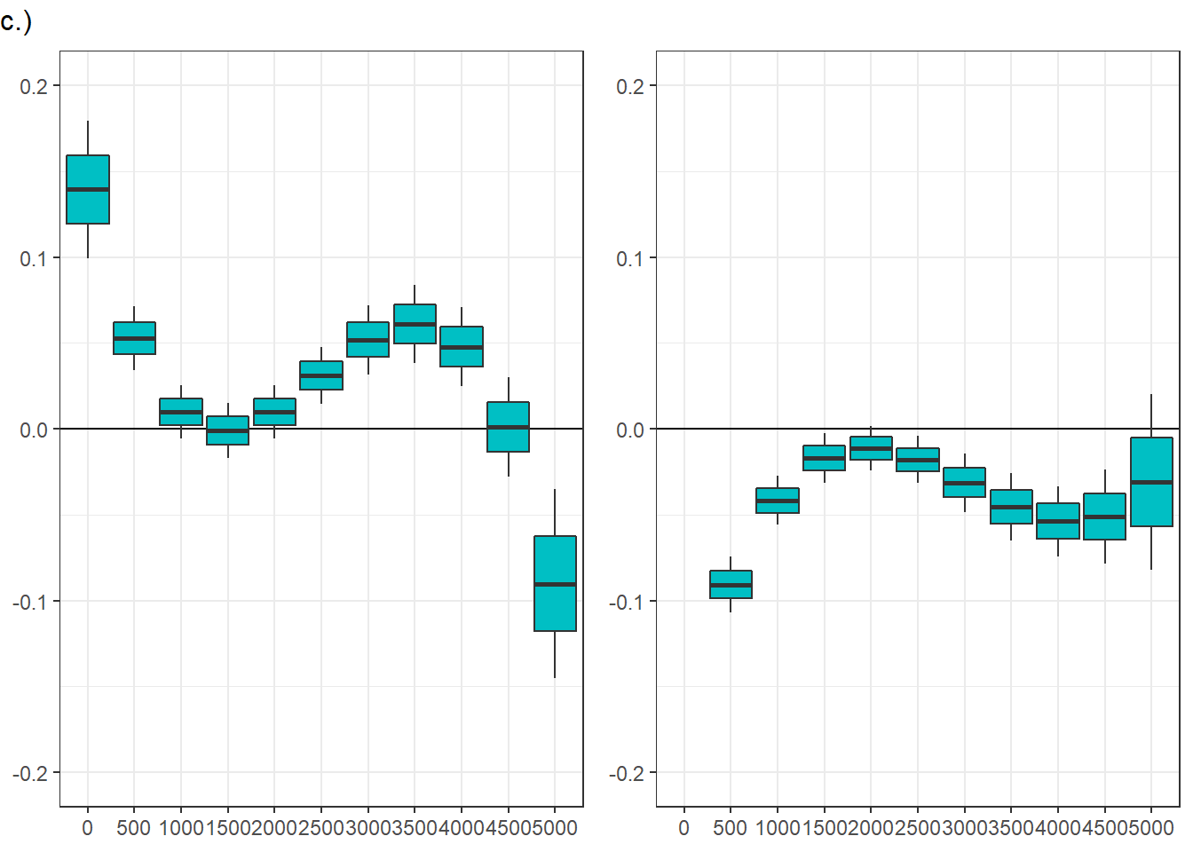
 vid_social ts.scene rpd_z.trend      SE  df asymp.LCL asymp.UCL
 FALSE          1000     -0.0398 0.00791 Inf  -0.05535 -2.43e-02
  TRUE          1000      0.0154 0.00957 Inf  -0.00338  3.41e-02
 FALSE          3000      0.0454 0.01021 Inf   0.02536  6.54e-02
  TRUE          3000     -0.0232 0.01183 Inf  -0.04637 -5.16e-06

Results are averaged over the levels of: t1_diagnosis, t1_sex 
Degrees-of-freedom method: asymptotic 
Confidence level used: 0.95

pupillary response

Linear mixed model: pupillary response
	Sum Sq	df1	df2	F	p	p_adj
group	0.106	1	302.500	0.151	0.697	1.000
video category (VC)	14.198	1	81.703	20.217	0.000	0.000
time^1	1.601	1	68037.834	2.279	0.131	0.393
time^2	1.551	1	68040.486	2.208	0.137	0.411
time^3	1.152	1	68038.926	1.640	0.200	0.600
sex	0.453	1	303.632	0.645	0.423	1.000
age	0.155	1	311.883	0.220	0.639	1.000
perceptual IQ	2.080	1	312.154	2.962	0.086	0.258
ADHD inattention	0.317	1	308.934	0.451	0.502	1.000
anxiety	2.943	1	296.463	4.190	0.042	0.126
depression	1.521	1	298.733	2.165	0.142	0.426
accuracy	0.060	1	311.669	0.085	0.771	1.000
precision	0.056	1	329.173	0.080	0.778	1.000
center deviation	309.587	1	68301.078	440.827	0.000	0.000
group x VC	179.322	1	68289.663	255.340	0.000	0.000
group x time^1	0.328	1	68016.915	0.467	0.495	1.000
group x time^2	0.379	1	68019.287	0.539	0.463	1.000
group x time^3	0.308	1	68019.658	0.438	0.508	1.000
VC x time^1	1.279	1	68036.983	1.821	0.177	0.531
VC x time^2	1.180	1	68039.325	1.680	0.195	0.585
VC x time^3	1.632	1	68038.962	2.324	0.127	0.381
group x VC x time^1	7.120	1	68021.133	10.138	0.001	0.003
group x VC x time^2	6.847	1	68025.566	9.749	0.002	0.006
group x VC x time^3	5.528	1	68025.587	7.871	0.005	0.015

                    2.5 % 97.5 %
vid_socialTRUE 0.38  0.17   0.59

vid_social = FALSE:
 contrast      estimate     SE  df asymp.LCL asymp.UCL
 ASD - Control   0.0773 0.0319 Inf    0.0149     0.140

vid_social =  TRUE:
 contrast      estimate     SE  df asymp.LCL asymp.UCL
 ASD - Control  -0.0904 0.0323 Inf   -0.1538    -0.027

Results are averaged over the levels of: t1_sex 
Degrees-of-freedom method: asymptotic 
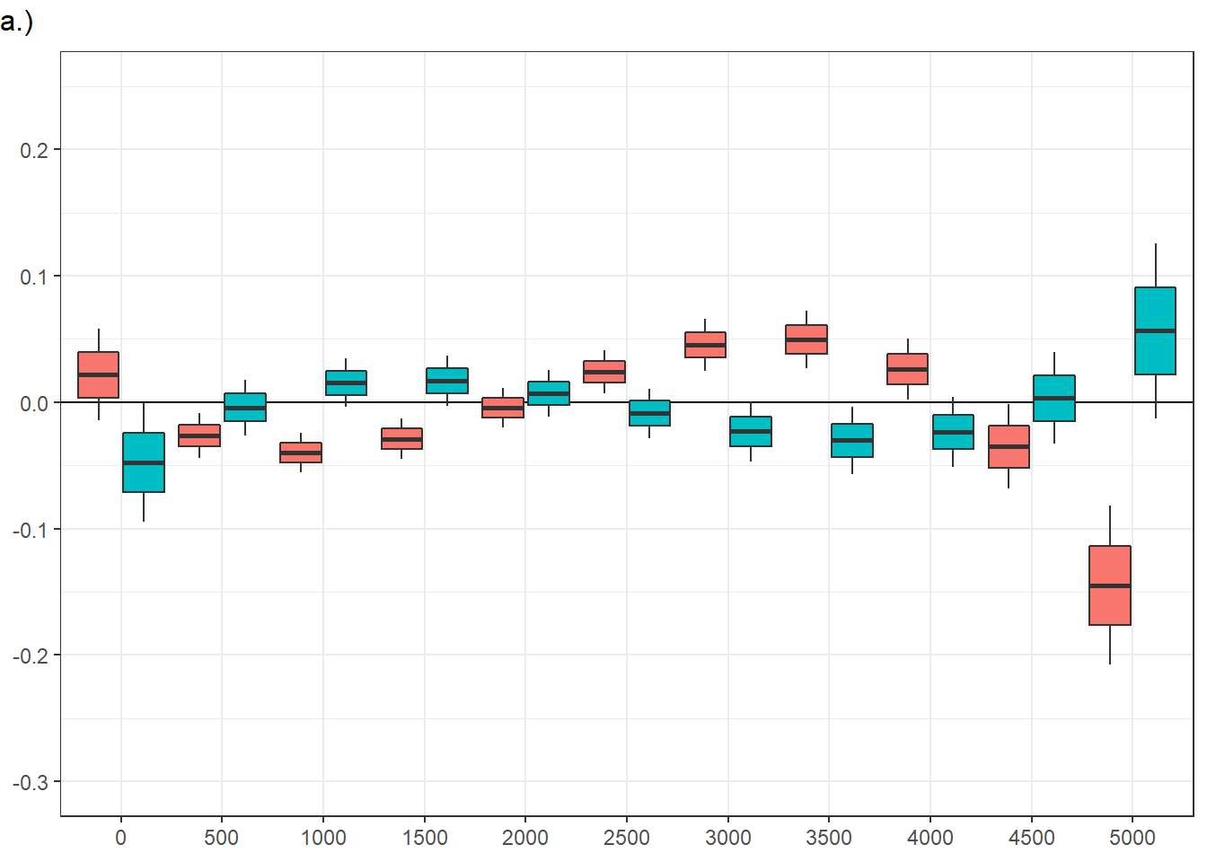
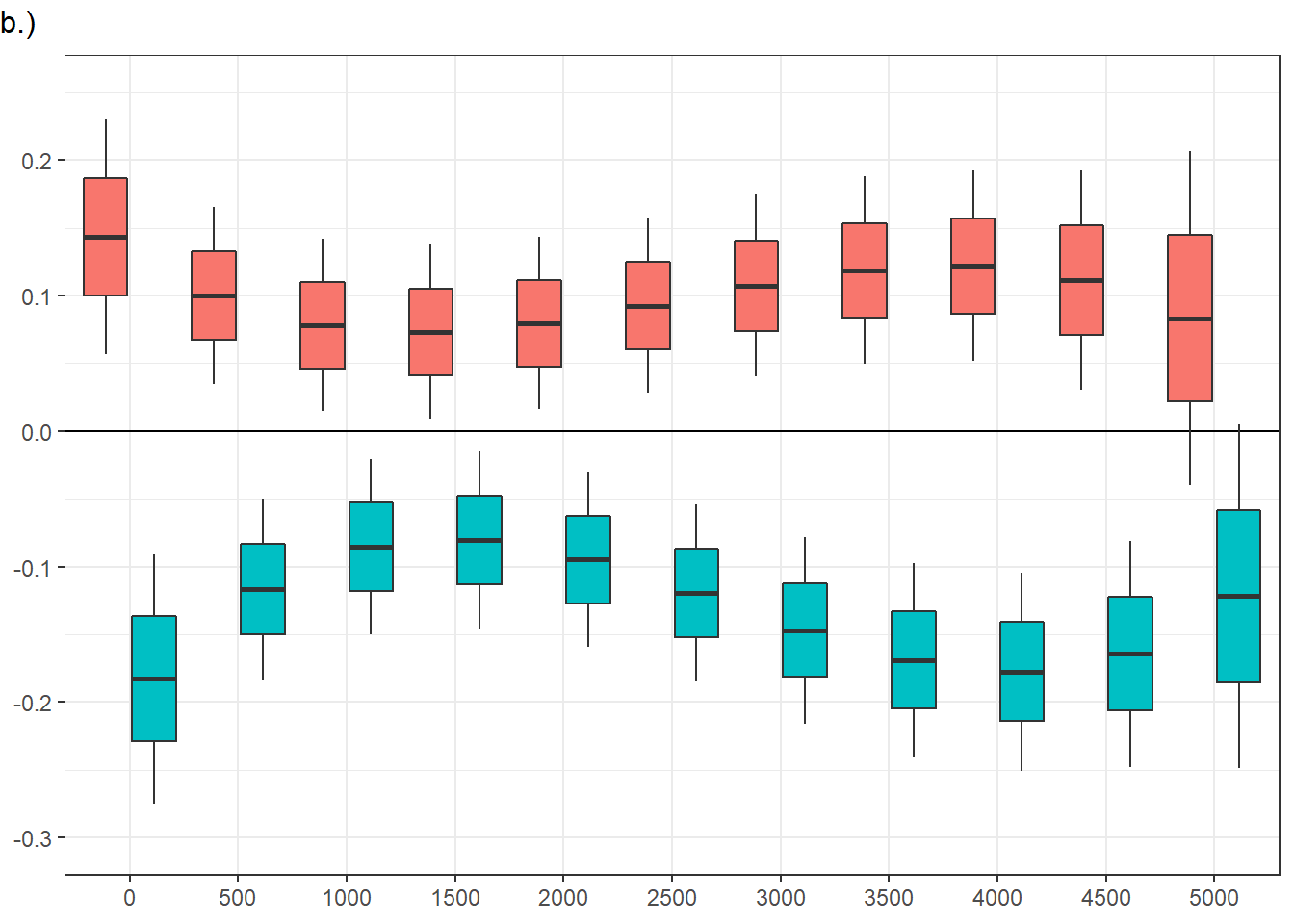
Confidence level used: 0.95

vid_social = FALSE, ts.scene =    0:
 contrast      estimate     SE  df asymp.LCL asymp.UCL
 ASD - Control   0.1435 0.0434 Inf    0.0584   0.22869

vid_social =  TRUE, ts.scene =    0:
 contrast      estimate     SE  df asymp.LCL asymp.UCL
 ASD - Control  -0.1829 0.0461 Inf   -0.2733  -0.09260

vid_social = FALSE, ts.scene = 1000:
 contrast      estimate     SE  df asymp.LCL asymp.UCL
 ASD - Control   0.0784 0.0319 Inf    0.0158   0.14095

vid_social =  TRUE, ts.scene = 1000:
 contrast      estimate     SE  df asymp.LCL asymp.UCL
 ASD - Control  -0.0853 0.0325 Inf   -0.1489  -0.02169

vid_social = FALSE, ts.scene = 2000:
 contrast      estimate     SE  df asymp.LCL asymp.UCL
 ASD - Control   0.0796 0.0318 Inf    0.0172   0.14191

vid_social =  TRUE, ts.scene = 2000:
 contrast      estimate     SE  df asymp.LCL asymp.UCL
 ASD - Control  -0.0948 0.0323 Inf   -0.1581  -0.03159

vid_social = FALSE, ts.scene = 3000:
 contrast      estimate     SE  df asymp.LCL asymp.UCL
 ASD - Control   0.1073 0.0336 Inf    0.0415   0.17317

vid_social =  TRUE, ts.scene = 3000:
 contrast      estimate     SE  df asymp.LCL asymp.UCL
 ASD - Control  -0.1470 0.0345 Inf   -0.2146  -0.07948

vid_social = FALSE, ts.scene = 4000:
 contrast      estimate     SE  df asymp.LCL asymp.UCL
 ASD - Control   0.1219 0.0352 Inf    0.0528   0.19090

vid_social =  TRUE, ts.scene = 4000:
 contrast      estimate     SE  df asymp.LCL asymp.UCL
 ASD - Control  -0.1775 0.0366 Inf   -0.2492  -0.10583

vid_social = FALSE, ts.scene = 5000:
 contrast      estimate     SE  df asymp.LCL asymp.UCL
 ASD - Control   0.0833 0.0615 Inf   -0.0372   0.20389

vid_social =  TRUE, ts.scene = 5000:
 contrast      estimate     SE  df asymp.LCL asymp.UCL
 ASD - Control  -0.1218 0.0636 Inf   -0.2465   0.00286

Results are averaged over the levels of: t1_sex 
Degrees-of-freedom method: asymptotic 
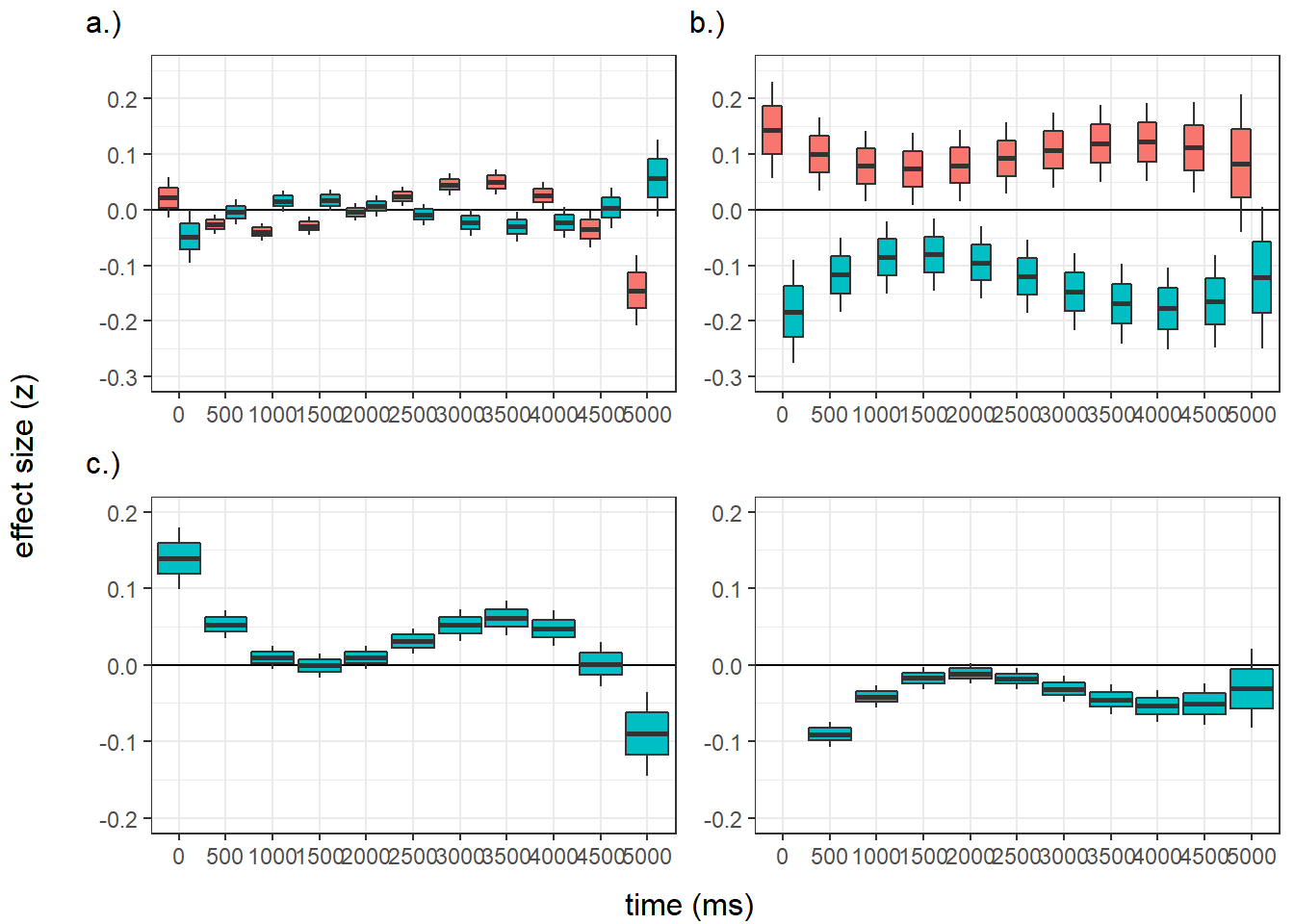
Confidence level used: 0.95

social attention

Linear mixed model: social attention without mediators
	Sum Sq	df1	df2	F	p	p_adj
group	3.353	1	290.061	5.948	0.015	0.045
time^1	493.544	1	30834.035	875.538	0.000	0.000
time^2	394.746	1	30838.669	700.271	0.000	0.000
time^3	336.955	1	30839.497	597.752	0.000	0.000
sex	2.085	1	288.649	3.699	0.055	0.165
age	13.937	1	294.063	24.724	0.000	0.000
perceptual IQ	6.424	1	297.287	11.396	0.001	0.003
ADHD inattention	1.152	1	293.236	2.044	0.154	0.462
anxiety	1.109	1	276.565	1.967	0.162	0.486
depression	1.928	1	282.287	3.420	0.065	0.195
accuracy	1.732	1	296.990	3.072	0.081	0.243
precision	1.029	1	322.288	1.825	0.178	0.534
center deviation	0.009	1	31080.415	0.016	0.898	1.000
group x time^1	0.001	1	30833.094	0.001	0.970	1.000
group x time^2	0.003	1	30838.662	0.006	0.938	1.000
group x time^3	0.007	1	30838.432	0.012	0.914	1.000

                         2.5 % 97.5 %
t1_diagnosisControl 0.08  0.02   0.15

Linear mixed model: social attention with motion salience and physical salience as mediators
	Sum Sq	df1	df2	F	p	p_adj
group	3.149	1	291.967	5.621	0.018	0.054
motion salience (MS)	54.143	1	30851.780	96.652	0.000	0.000
physical salience (PS)	16.781	1	30873.352	29.956	0.000	0.000
time^1	397.803	1	30825.838	710.130	0.000	0.000
time^2	317.004	1	30829.695	565.894	0.000	0.000
time^3	271.098	1	30829.610	483.944	0.000	0.000
sex	2.119	1	289.284	3.782	0.053	0.159
age	14.245	1	294.696	25.430	0.000	0.000
perceptual IQ	6.448	1	297.959	11.510	0.001	0.003
ADHD inattention	1.169	1	293.874	2.086	0.150	0.450
anxiety	1.139	1	277.212	2.033	0.155	0.465
depression	1.960	1	282.915	3.499	0.062	0.186
accuracy	1.733	1	297.622	3.094	0.080	0.240
precision	0.996	1	322.964	1.778	0.183	0.549
center deviation	0.048	1	31060.673	0.086	0.770	1.000
group x MS	1.106	1	30846.537	1.974	0.160	0.480
group x PS	0.001	1	30888.345	0.002	0.968	1.000
group x time^1	0.008	1	30824.269	0.014	0.904	1.000
group x time^2	0.020	1	30828.970	0.037	0.848	1.000
group x time^3	0.021	1	30827.765	0.037	0.847	1.000
MS x time^1	21.814	1	30845.550	38.940	0.000	0.000
MS x time^2	12.503	1	30846.586	22.320	0.000	0.000
MS x time^3	7.808	1	30846.059	13.938	0.000	0.000
PS x time^1	21.357	1	30836.977	38.124	0.000	0.000
PS x time^2	21.067	1	30830.198	37.608	0.000	0.000
PS x time^3	20.362	1	30826.496	36.350	0.000	0.000
group x MS x time^1	0.046	1	30863.106	0.083	0.773	1.000
group x MS x time^2	0.001	1	30865.920	0.002	0.965	1.000
group x MS x time^3	0.051	1	30864.065	0.091	0.764	1.000
group x PS x time^1	0.010	1	30835.669	0.019	0.892	1.000
group x PS x time^2	0.004	1	30829.768	0.007	0.936	1.000
group x PS x time^3	0.002	1	30826.237	0.004	0.950	1.000

      2.5 % 97.5 %

      2.5 % 97.5 %

Linear mixed model: social attention with pupillary response as mediator
	Sum Sq	df1	df2	F	p	p_adj
group	2.618	1	296.947	4.648	0.032	0.096
pupillary response (PR)	2.462	1	29775.259	4.371	0.037	0.111
time^1	483.326	1	30829.336	858.029	0.000	0.000
time^2	385.100	1	30836.443	683.653	0.000	0.000
time^3	327.715	1	30839.485	581.778	0.000	0.000
sex	2.060	1	289.223	3.657	0.057	0.171
age	13.823	1	294.674	24.539	0.000	0.000
perceptual IQ	6.631	1	297.972	11.771	0.001	0.003
ADHD inattention	1.203	1	293.747	2.136	0.145	0.435
anxiety	1.064	1	277.087	1.889	0.170	0.510
depression	1.842	1	282.756	3.271	0.072	0.216
accuracy	1.729	1	297.376	3.070	0.081	0.243
precision	1.057	1	322.695	1.877	0.172	0.516
center deviation	0.000	1	31074.634	0.001	0.981	1.000
group x PR	4.068	1	30115.935	7.221	0.007	0.021
group x time^1	0.137	1	30829.036	0.243	0.622	1.000
group x time^2	0.170	1	30836.819	0.302	0.583	1.000
group x time^3	0.185	1	30839.276	0.329	0.567	1.000
PR x time^1	7.388	1	30836.368	13.115	0.000	0.000
PR x time^2	6.289	1	30842.004	11.164	0.001	0.003
PR x time^3	5.550	1	30844.364	9.853	0.002	0.006
group x PR x time^1	0.322	1	30834.579	0.572	0.449	1.000
group x PR x time^2	0.221	1	30839.948	0.392	0.531	1.000
group x PR x time^3	0.222	1	30842.416	0.393	0.530	1.000

 t1_diagnosis rpd_z.trend      SE  df asymp.LCL asymp.UCL
 ASD              -0.0397 0.01203 Inf   -0.0632  -0.01607
 Control          -0.0142 0.00991 Inf   -0.0336   0.00524

Results are averaged over the levels of: t1_sex 
Degrees-of-freedom method: asymptotic 
Confidence level used: 0.95

Linear mixed model: social attention with pupillary components as mediator
	Sum Sq	df1	df2	F	p	p_adj
group	2.819	1	296.172	4.850	0.028	0.084
early pupillary comp. (PC1)	22.452	1	30931.252	38.635	0.000	0.000
late pupillary comp. (PC2)	10.639	1	31012.716	18.308	0.000	0.000
sex	2.175	1	288.391	3.743	0.054	0.162
age	13.875	1	293.999	23.876	0.000	0.000
perceptual IQ	6.746	1	297.265	11.608	0.001	0.003
ADHD inattention	1.369	1	293.051	2.355	0.126	0.378
anxiety	1.007	1	276.027	1.733	0.189	0.567
depression	1.917	1	281.833	3.299	0.070	0.210
accuracy	1.738	1	296.766	2.990	0.085	0.255
precision	1.137	1	322.412	1.957	0.163	0.489
center deviation	0.031	1	31087.730	0.053	0.819	1.000
group x PC1	0.907	1	30988.299	1.561	0.211	0.633
group x PC2	2.198	1	31007.773	3.782	0.052	0.156

                2.5 % 97.5 %
rpd_RC1_z -0.04 -0.05  -0.02

               2.5 % 97.5 %
rpd_RC2_z 0.01     0   0.03

panel figure - temporal effects

png 
  2

R version 3.6.1 (2019-07-05)
Platform: x86_64-w64-mingw32/x64 (64-bit)
Running under: Windows 10 x64 (build 19043)

Matrix products: default

locale:
[1] LC_COLLATE=German_Germany.1252  LC_CTYPE=German_Germany.1252   
[3] LC_MONETARY=German_Germany.1252 LC_NUMERIC=C                   
[5] LC_TIME=German_Germany.1252    

attached base packages:
[1] stats     graphics  grDevices utils     datasets  methods   base     

other attached packages:
 [1] simr_1.0.5       missMDA_1.18     psych_1.9.12.31  MuMIn_1.43.17   
 [5] emmeans_1.4.3.01 lmerTest_3.1-2   lme4_1.1-23      Matrix_1.2-18   
 [9] kableExtra_1.3.1 gridExtra_2.3    sjmisc_2.8.5     sjPlot_2.8.5    
[13] ggplot2_3.2.1    reshape2_1.4.3   R.matlab_3.6.2   MatchIt_3.0.2   
[17] Gmisc_1.11.0     htmlTable_2.1.0  Rcpp_1.0.3       mice_3.7.0      
[21] lattice_0.20-38  zoo_1.8-6        readxl_1.3.1    

loaded via a namespace (and not attached):
  [1] backports_1.1.5      Hmisc_4.3-0          workflowr_1.6.2     
  [4] plyr_1.8.5           lazyeval_0.2.2       splines_3.6.1       
  [7] RLRsim_3.1-3         digest_0.6.23        foreach_1.5.1       
 [10] htmltools_0.4.0      magrittr_1.5         checkmate_1.9.4     
 [13] cluster_2.1.0        doParallel_1.0.16    openxlsx_4.1.4      
 [16] modelr_0.1.5         R.utils_2.9.2        jpeg_0.1-8.1        
 [19] colorspace_1.4-1     rvest_0.3.5          ggrepel_0.8.1       
 [22] haven_2.2.0          pan_1.6              xfun_0.11           
 [25] dplyr_1.0.2          crayon_1.3.4         survival_3.1-8      
 [28] iterators_1.0.12     glue_1.4.2           gtable_0.3.0        
 [31] webshot_0.5.2        sjstats_0.18.0       car_3.0-6           
 [34] jomo_2.6-10          abind_1.4-5          scales_1.1.0        
 [37] mvtnorm_1.0-11       ggeffects_0.16.0     plotrix_3.7-7       
 [40] viridisLite_0.3.0    xtable_1.8-4         performance_0.5.0   
 [43] flashClust_1.01-2    foreign_0.8-74       Formula_1.2-3       
 [46] stats4_3.6.1         DT_0.11              htmlwidgets_1.5.1   
 [49] httr_1.4.1           RColorBrewer_1.1-2   acepack_1.4.1       
 [52] ellipsis_0.3.0       pkgconfig_2.0.3      XML_3.99-0.3        
 [55] R.methodsS3_1.7.1    binom_1.1-1          nnet_7.3-12         
 [58] tidyselect_1.1.0     rlang_0.4.8          later_1.0.0         
 [61] effectsize_0.0.1     munsell_0.5.0        cellranger_1.1.0    
 [64] tools_3.6.1          generics_0.0.2       sjlabelled_1.1.6    
 [67] broom_0.7.2          evaluate_0.14        stringr_1.4.0       
 [70] yaml_2.2.0           knitr_1.26           fs_1.3.1            
 [73] zip_2.0.4            forestplot_1.10      purrr_0.3.3         
 [76] mitml_0.3-7          nlme_3.1-143         R.oo_1.23.0         
 [79] leaps_3.1            xml2_1.2.2           pbkrtest_0.4-7      
 [82] compiler_3.6.1       rstudioapi_0.10      curl_4.3            
 [85] png_0.1-7            tibble_3.0.4         statmod_1.4.34      
 [88] stringi_1.4.5        highr_0.8            parameters_0.8.5    
 [91] forcats_0.4.0        nloptr_1.2.1         vctrs_0.3.4         
 [94] pillar_1.4.3         lifecycle_0.2.0      estimability_1.3    
 [97] data.table_1.12.8    insight_0.9.6        httpuv_1.5.2        
[100] R6_2.4.1             latticeExtra_0.6-29  promises_1.1.0      
[103] rio_0.5.16           codetools_0.2-16     boot_1.3-24         
[106] MASS_7.3-51.5        rprojroot_1.3-2      withr_2.1.2         
[109] mnormt_1.5-5         hms_0.5.3            mgcv_1.8-31         
[112] bayestestR_0.7.2     parallel_3.6.1       grid_3.6.1          
[115] rpart_4.1-15         tidyr_1.0.0          coda_0.19-4         
[118] minqa_1.2.4          rmarkdown_2.0        carData_3.0-3       
[121] git2r_0.26.1         numDeriv_2016.8-1.1  scatterplot3d_0.3-41
[124] lubridate_1.7.9      base64enc_0.1-3      FactoMineR_2.4

data_analysis_salience

Nico Bast

13 9 2021