Iterative Comparison
Last updated: 2023-04-10
Checks: 7 0
Knit directory: dgrp-starve/
This reproducible R Markdown analysis was created with workflowr (version 1.7.0). The Checks tab describes the reproducibility checks that were applied when the results were created. The Past versions tab lists the development history.
Great! Since the R Markdown file has been committed to the Git repository, you know the exact version of the code that produced these results.
Great job! The global environment was empty. Objects defined in the global environment can affect the analysis in your R Markdown file in unknown ways. For reproduciblity it’s best to always run the code in an empty environment.
The command set.seed(20221101) was run prior to running
the code in the R Markdown file. Setting a seed ensures that any results
that rely on randomness, e.g. subsampling or permutations, are
reproducible.
Great job! Recording the operating system, R version, and package versions is critical for reproducibility.
Nice! There were no cached chunks for this analysis, so you can be confident that you successfully produced the results during this run.
Great job! Using relative paths to the files within your workflowr project makes it easier to run your code on other machines.
Great! You are using Git for version control. Tracking code development and connecting the code version to the results is critical for reproducibility.
The results in this page were generated with repository version 1319ab9. See the Past versions tab to see a history of the changes made to the R Markdown and HTML files.
Note that you need to be careful to ensure that all relevant files for
the analysis have been committed to Git prior to generating the results
(you can use wflow_publish or
wflow_git_commit). workflowr only checks the R Markdown
file, but you know if there are other scripts or data files that it
depends on. Below is the status of the Git repository when the results
were generated:
Ignored files:
    Ignored:    code/snake/
    Ignored:    data/snake/

Untracked files:
    Untracked:  .snakemake/
    Untracked:  ETA_1_parBayesC.dat
    Untracked:  analysis/linearReg.Rmd
    Untracked:  bglr-f.R
    Untracked:  code/PCA/
    Untracked:  code/data-prep/
    Untracked:  code/fabio/
    Untracked:  code/gBayesC.R
    Untracked:  code/id_bank_creation.R
    Untracked:  code/intro-starve/
    Untracked:  code/methodComp/
    Untracked:  code/regress/
    Untracked:  data/bayesF.rds
    Untracked:  data/bayesM.rds
    Untracked:  data/bglr-f-130k.rds
    Untracked:  data/bglr-f.rds
    Untracked:  data/bglr-m-130k.rds
    Untracked:  data/bglr-m.rds
    Untracked:  data/corLoop-f-minus.rds
    Untracked:  data/corLoop-f.rds
    Untracked:  data/corLoop-m-Minus.rds
    Untracked:  data/corLoop-m-minus.rds
    Untracked:  data/corLoop-m.rds
    Untracked:  data/fRegress.txt
    Untracked:  data/fRegress_adj.txt
    Untracked:  data/fm.burglar
    Untracked:  data/gbayesC-f.Rds
    Untracked:  data/gbayesC-m.Rds
    Untracked:  data/gbayesC.Rds
    Untracked:  data/gbayes_100k-f.Rds
    Untracked:  data/gbayes_100k-m.Rds
    Untracked:  data/goGroups.txt
    Untracked:  data/id_bank
    Untracked:  data/id_bank.Rds
    Untracked:  data/mPart.txt
    Untracked:  data/mRegress.txt
    Untracked:  data/mRegress_adj.txt
    Untracked:  data/multiReg.rData
    Untracked:  data/pheno_f
    Untracked:  data/pheno_m
    Untracked:  data/starve-f.txt
    Untracked:  data/starve-m.txt
    Untracked:  data/xp-f.txt
    Untracked:  data/xp-m.txt
    Untracked:  data/xp_f
    Untracked:  data/xp_m
    Untracked:  data/y_save.txt
    Untracked:  figure/
    Untracked:  filesnake1
    Untracked:  filesnake4_3
    Untracked:  junk/
    Untracked:  m_starvation
    Untracked:  mu.dat
    Untracked:  notes/
    Untracked:  snake/
    Untracked:  varE.dat

Unstaged changes:
    Deleted:    analysis/gremlo.R
    Modified:   analysis/index.Rmd
    Deleted:    analysis/methodComp-f.Rmd
    Deleted:    analysis/methodComp-m.Rmd
    Deleted:    analysis/stepwise-f.Rmd
    Deleted:    analysis/stepwise-m.Rmd
    Deleted:    analysis/testing.R
    Deleted:    analysis/tips.Rmd
    Modified:   analysis/trace.Rmd
    Deleted:    code/baseScript-lineComp.R
    Deleted:    code/combineSNP.R
    Deleted:    code/four-comp.76979.err
    Deleted:    code/four-comp.76979.out
    Deleted:    code/four-comp.sbatch
    Deleted:    code/fourLinePrep.R
    Deleted:    code/line_avgMinus.R
    Deleted:    code/line_avgPlus.R
    Deleted:    code/line_difMinus.R
    Deleted:    code/line_difPlus.R
    Deleted:    code/snpGene.R
    Deleted:    code/starveDataPrep.R
Note that any generated files, e.g. HTML, png, CSS, etc., are not included in this status report because it is ok for generated content to have uncommitted changes.
These are the previous versions of the repository in which changes were
made to the R Markdown (analysis/methodComp.Rmd) and HTML
(docs/methodComp.html) files. If you’ve configured a remote
Git repository (see ?wflow_git_remote), click on the
hyperlinks in the table below to view the files as they were in that
past version.
| File | Version | Author | Date | Message |
|---|---|---|---|---|
| Rmd | 1319ab9 | nklimko | 2023-04-10 | wflow_publish("analysis/methodComp.Rmd") |
| html | a893dba | nklimko | 2023-04-02 | Build site. |
| html | f2074cb | nklimko | 2023-03-28 | Build site. |
| Rmd | aefe7e0 | nklimko | 2023-03-28 | wflow_publish("analysis/methodComp.Rmd") |
| html | 7671e99 | nklimko | 2023-03-27 | Build site. |
| Rmd | be6876c | nklimko | 2023-03-27 | wflow_publish("analysis/methodComp.Rmd") |
| html | 5b9c5a5 | nklimko | 2023-03-27 | Build site. |
| html | af523cd | nklimko | 2023-03-27 | Build site. |
| Rmd | 2afd953 | nklimko | 2023-03-27 | wflow_publish("analysis/methodComp.Rmd") |
| html | f55e150 | nklimko | 2023-03-21 | Build site. |
| Rmd | 39a0792 | nklimko | 2023-03-21 | wflow_publish("analysis/methodComp.Rmd") |
| html | 29ccf74 | nklimko | 2023-03-21 | Build site. |
| Rmd | 87d7e5c | nklimko | 2023-03-21 | wflow_publish("analysis/methodComp.Rmd") |
The overarching goal of this process is to predict the phenotype for starvation resistance, a continuous trait, by using gene expression data, another continuous trait. This is done using k-fold cross validation to create models based on a subset of the data and calculating the correlation of that model with the remaining partition. By repeating this process multiple times with different training and testing partitions, model bias can be significantly reduced and allows for calculation of average correlation coefficients for each model. The primary difference between the methods in question is the prior distribution used.
#loop count and data limit
iter <- 50

#ggplot holder list
gg <- vector(mode='list', length=6)

# result storage elements
fit_greml <- vector(mode='list', length=iter)
fit_gbayesC <- vector(mode='list', length=iter)
fit_varbvs <- vector(mode='list', length=iter)
fit_glmnet <- vector(mode='list', length=iter)
fit_bglr <- vector(mode='list', length=iter)
The first main set of data used for this analysis is a matrix of gene expression by DGRP line matched to raw starvation resistance. A second cluster of data sets provided by the Morgante Lab includes information on Wolbachia infection status and inversion status by line along with functions to adjust phenotypic values based on these two factors.
 #wolb infection and inversion status data with phenotype adjustment function
load("/data2/morgante_lab/data/dgrp/misc/adjustData.RData")

  #expression data matched to line and starvation phenotype
  xp_f <- fread("data/xp-f.txt")

 # xp_m <- fread("data/xp-m.txt")

  #setwd("C:/Users/noahk/OneDrive/Desktop/amogus")
  #getwd()

  #create matrix of only gene expression, trims line and starvation
  X <- as.matrix(xp_f[,3:11340])
  rownames(X) <- xp_f[,line]
  W <- scale(X)

  y_temp <- xp_f[,starvation]
  dat <- data.frame(id=xp_f[,line], y=y_temp)
  y <- adjustPheno(dat, "starvation")


#model to solve for, vector of ones
mu <- matrix(rep(1, length(y)), ncol=1)
#names(mu) <- paste0("line", 1:length(mu))
rownames(mu) <- xp_f[,line]
TRM <- tcrossprod(W)/ncol(W)

# k-fold parameters
n <- length(y)
fold <- 5
The matrix containing only gene expression by line data was then scaled to an absolute max of 1. along with this, a Translation Relationship Matrix was generated by taking the crossproduct of the scaled expression matrix and scaling it down by the number of genes.
5 was chosen for k-fold cross validation resulting in 39 lines per validation set and 159 lines per training set.
The following methods are currently implemented:
qgg::greml - Genomic Restricted Maximum Likelihood Estimation using Best Linear Unbiased Predictor. GREML uses a Gaussian prior distribution, performing the least shrinkage and no variable selection.
glmnet - glmnet uses LASSO, or least absolute shrinkage and selection operator. Bayesian LASSO uses a thick-tailed prior which performs greater shrinkage towards the mean than a Gaussian distribution.
qgg::gbayes - BayesC has been implemented using this command. BayesC uses a spike-slab prior which performs variable selection. This intentionally sets the effect of some genes expressed to zero which models the idea that some genes have no effect on the given trait.
varbvs - Bayesian variable selection performs variable selection using another spike-slab prior. This method avoids Markov Chain Monte Carlo methods by approximating the posterior distribution to reduce computational resources.
BGLR - Bayesian General Linear Regression has the capability to perform BayesC linear regression using a Gibbs Sampler.
ids <- readRDS("data/id_bank.Rds")

registerDoParallel(cores = 1)

iter <- 1

i <- 1

corLoop <- foreach(i=1:iter) %dopar% {

  #result holder
  corResult <- rep(0, 5)

  #setup train and test sets with trait vectors
  #test_IDs <- sample(1:n, as.integer(n / fold))

  test_IDs <- unlist(ids[i])

  W_train <- W[-test_IDs,]
  W_test <- W[test_IDs,]
  y_train <- y[-test_IDs]
  y_test <- y[test_IDs]

   ### BGLR
  fitBGLR <- BGLR::BGLR(y_train, response_type = "gaussian", a=NULL, b=NULL,ETA = list(list(X=W_train, model="BayesC")), nIter = 500, burnIn = 200)

  y_calc <- predict(fitBGLR, W_test)

  corResult[5] <- cor(y_test, y_calc)

  length(y_calc)
  length(y_test)

  #Overall result
  corResult

}


corLoop <- foreach(i=1:iter) %dopar% {

  #result holder
  corResult <- rep(0, 5)

  #setup train and test sets with trait vectors
  #test_IDs <- sample(1:n, as.integer(n / fold))

  test_IDs <- unlist(ids[i])

  W_train <- W[-test_IDs,]
  W_test <- W[test_IDs,]
  y_train <- y[-test_IDs]
  y_test <- y[test_IDs]


  ### QGG::GREML
  fitGreml <- qgg::greml(y=y, X=mu, GRM=list(A=TRM), validate = matrix(test_IDs,ncol=1), verbose=FALSE)

  corResult[1] <- fitGreml$accuracy$Corr

  ### QGG::GBAYES-C
  fitC <- qgg::gbayes(y=y_train, W=W_train, method="bayesC", scaleY=FALSE, nit=50000, nburn=20000)

  # \hat{y}_test = W_{test} * \hat{b} + \hat{mu}
  y_calc <- W_test %*% fitC$b + mean(y_train)
  corResult[2] <- cor(y_test, y_calc)

  ### VARBVS
  fitVarb <- varbvs::varbvs(X = W_train, NULL, y=y_train, family = "gaussian", logodds=seq(-3.5,-1,0.1), sa = 1, verbose=TRUE)

  y_calc <- predict(fitVarb, X=W_test)
  corResult[3] <- cor(y_test, y_calc)

  ### GLMNET::LASSO
  fitlm <- glmnet::cv.glmnet(x=W_train, y=y_train, alpha=1)

  y_calc <- predict(fitlm, W_test, s="lambda.min")
  corResult[4] <- cor(y_test, y_calc)

  ### BGLR
  fitBGLR <- BGLR::BGLR(y_train, response_type = "gaussian", a=NULL, b=NULL,ETA = list(list(X=W_train, model="BayesC")), nIter = 50000, burnIn = 20000)

  y_calc <- predict(fitBGLR, W_test)
  corResult[5] <- cor(y_test, y_calc)

  #Overall result
  corResult

}
iter <- 50
# results loaded from correlation loop structure
bayesF <- readRDS("data/bayesF.rds")
corLoop <- readRDS("data/corLoop-f-minus.rds")
bglrLoop <- readRDS("data/bglr-f-130k.rds")
for(i in 1:iter){
fit_greml[[i]] <- corLoop[[i]][1]
fit_gbayesC[[i]] <- bayesF[[i]][1]
fit_varbvs[[i]] <- corLoop[[i]][2]
fit_glmnet[[i]] <- corLoop[[i]][3]
fit_bglr[[i]] <- bglrLoop[[i]][5]
}
temp <- c(unlist(fit_greml), unlist(fit_gbayesC), unlist(fit_varbvs), unlist(fit_glmnet), unlist(fit_bglr))
label <- c(rep("greml", iter), rep("gBayesC", iter), rep("varbvs", iter), rep("glmnet", iter), rep("bglr", iter))
data <- data.table(cor=as.numeric(temp), method=label)
gg[[1]] <- ggplot(data, aes(x=method, y=cor, fill=method)) +
geom_boxplot() +
ggtitle("Female Correlations Boxplot") +
labs(x="Method", y="Correlation Coefficient") +
stat_summary(fun=mean, color="black", geom="point",
shape=18, size=3, show.legend=FALSE) # results loaded from correlation loop structure
bayesM <- readRDS("data/bayesM.rds")
corLoop <- readRDS("data/corLoop-m-Minus.rds")
bglrLoop <- readRDS("data/bglr-m-130k.rds")
for(i in 1:iter){
fit_greml[[i]] <- corLoop[[i]][1]
fit_gbayesC[[i]] <- bayesM[[i]][1]
fit_varbvs[[i]] <- corLoop[[i]][2]
fit_glmnet[[i]] <- corLoop[[i]][3]
fit_bglr[[i]] <- bglrLoop[[i]][5]
}
temp <- c(unlist(fit_greml), unlist(fit_gbayesC), unlist(fit_varbvs), unlist(fit_glmnet), unlist(fit_bglr))
label <- c(rep("greml", iter), rep("gBayesC", iter), rep("varbvs", iter), rep("glmnet", iter), rep("bglr", iter))
data <- data.table(cor=as.numeric(temp), method=label)
gg[[2]] <- ggplot(data, aes(x=method, y=cor, fill=method)) +
geom_boxplot() +
ggtitle("Male Correlations Boxplot") +
labs(x="Method", y="Correlation Coefficient") +
stat_summary(fun=mean, color="black", geom="point",
shape=18, size=3, show.legend=FALSE) ### FEMALE
bglr <- readRDS("snake/data/2_cor/bglr_f_starvation.Rds")
glmnetLasso <- readRDS("snake/data/2_cor/glmnetLasso_f_starvation.Rds")
varbvs <- readRDS("snake/data/2_cor/varbvs_f_starvation.Rds")
temp <- c(varbvs, glmnetLasso, bglr)
label <- c(rep("varbvs", iter), rep("glmnetLasso", iter), rep("bglr", iter))
data <- data.table(cor=as.numeric(temp), method=label)
gg[[3]] <- ggplot(data, aes(x=method, y=cor, fill=method)) +
geom_boxplot() +
ggtitle("Female Correlations Boxplot") +
labs(x="Method", y="Correlation Coefficient") +
stat_summary(fun=mean, color="black", geom="point",
shape=18, size=3, show.legend=FALSE)
### MALE
bglr <- readRDS("snake/data/2_cor/bglr_m_starvation.Rds")
glmnetLasso <- readRDS("snake/data/2_cor/glmnetLasso_m_starvation.Rds")
varbvs <- readRDS("snake/data/2_cor/varbvs_m_starvation.Rds")
temp <- c(varbvs, glmnetLasso, bglr)
label <- c(rep("varbvs", iter), rep("glmnetLasso", iter), rep("bglr", iter))
data <- data.table(cor=as.numeric(temp), method=label)
gg[[4]] <- ggplot(data, aes(x=method, y=cor, fill=method)) +
geom_boxplot() +
ggtitle("Male Correlations Boxplot") +
labs(x="Method", y="Correlation Coefficient") +
stat_summary(fun=mean, color="black", geom="point",
shape=18, size=3, show.legend=FALSE)Correlation Coefficient Boxplots
plot_grid(gg[[1]],gg[[2]], ncol=2)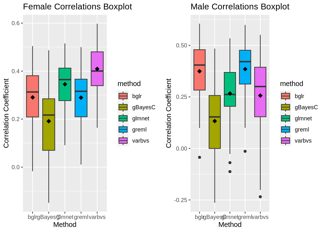
plot_grid(gg[[3]],gg[[4]], ncol=2)Warning: Removed 2 rows containing non-finite values (`stat_boxplot()`).Warning: Removed 2 rows containing non-finite values (`stat_summary()`).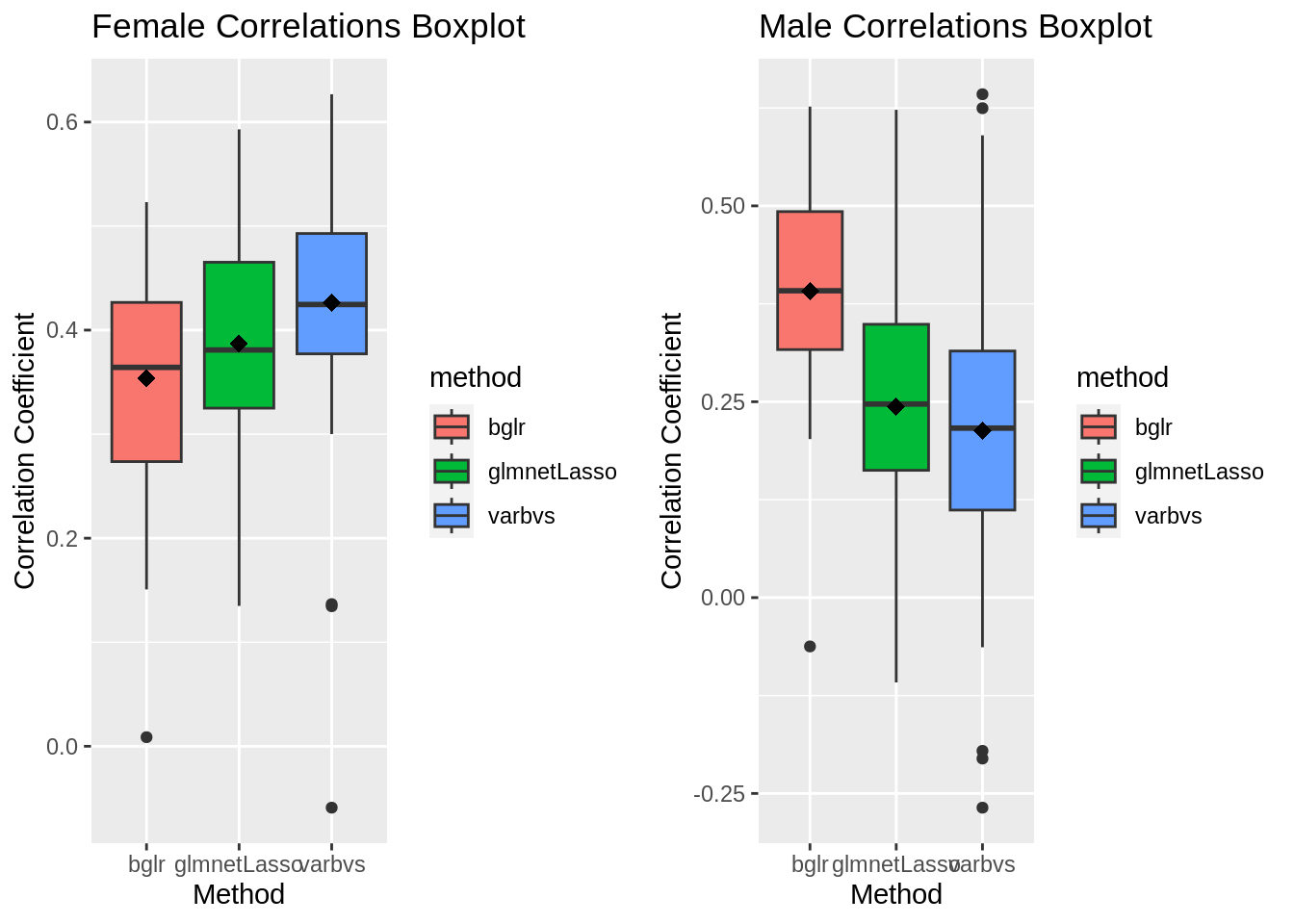
sessionInfo()R version 4.1.2 (2021-11-01)
Platform: x86_64-pc-linux-gnu (64-bit)
Running under: Rocky Linux 8.5 (Green Obsidian)
Matrix products: default
BLAS/LAPACK: /opt/ohpc/pub/libs/gnu9/openblas/0.3.7/lib/libopenblasp-r0.3.7.so
locale:
[1] LC_CTYPE=en_US.UTF-8 LC_NUMERIC=C
[3] LC_TIME=en_US.UTF-8 LC_COLLATE=en_US.UTF-8
[5] LC_MONETARY=en_US.UTF-8 LC_MESSAGES=en_US.UTF-8
[7] LC_PAPER=en_US.UTF-8 LC_NAME=C
[9] LC_ADDRESS=C LC_TELEPHONE=C
[11] LC_MEASUREMENT=en_US.UTF-8 LC_IDENTIFICATION=C
attached base packages:
[1] parallel stats graphics grDevices utils datasets methods
[8] base
other attached packages:
[1] BGLR_1.1.0 glmnet_4.1-6 Matrix_1.5-3 varbvs_2.5-16
[5] qgg_1.1.1 doParallel_1.0.17 iterators_1.0.14 foreach_1.5.2
[9] qqman_0.1.8 cowplot_1.1.1 ggplot2_3.4.1 data.table_1.14.8
[13] dplyr_1.1.0 workflowr_1.7.0
loaded via a namespace (and not attached):
[1] httr_1.4.5 sass_0.4.5 nor1mix_1.3-0
[4] jsonlite_1.8.4 splines_4.1.2 bslib_0.4.2
[7] getPass_0.2-2 statmod_1.5.0 highr_0.10
[10] latticeExtra_0.6-30 yaml_2.3.7 pillar_1.8.1
[13] lattice_0.20-45 quantreg_5.94 glue_1.6.2
[16] digest_0.6.31 RColorBrewer_1.1-3 promises_1.2.0.1
[19] colorspace_2.1-0 htmltools_0.5.4 httpuv_1.6.9
[22] pkgconfig_2.0.3 SparseM_1.81 calibrate_1.7.7
[25] scales_1.2.1 processx_3.8.0 whisker_0.4.1
[28] jpeg_0.1-10 later_1.3.0 MatrixModels_0.5-1
[31] git2r_0.31.0 tibble_3.2.0 farver_2.1.1
[34] generics_0.1.3 cachem_1.0.7 withr_2.5.0
[37] cli_3.6.0 survival_3.5-5 magrittr_2.0.3
[40] deldir_1.0-6 mcmc_0.9-7 evaluate_0.20
[43] ps_1.7.2 fs_1.6.1 fansi_1.0.4
[46] MASS_7.3-58.3 truncnorm_1.0-9 tools_4.1.2
[49] lifecycle_1.0.3 stringr_1.5.0 MCMCpack_1.6-3
[52] interp_1.1-3 munsell_0.5.0 callr_3.7.3
[55] compiler_4.1.2 jquerylib_0.1.4 rlang_1.1.0
[58] grid_4.1.2 rstudioapi_0.14 labeling_0.4.2
[61] rmarkdown_2.20 gtable_0.3.1 codetools_0.2-19
[64] R6_2.5.1 knitr_1.42 fastmap_1.1.1
[67] utf8_1.2.3 rprojroot_2.0.3 shape_1.4.6
[70] stringi_1.7.12 Rcpp_1.0.10 vctrs_0.5.2
[73] png_0.1-8 tidyselect_1.2.0 xfun_0.37
[76] coda_0.19-4