Monte Carlo Simulation
R. Noah Padgett
2020-10-22
Last updated: 2020-10-23
Checks: 6 1
Knit directory: laplace-local-fit/
This reproducible R Markdown analysis was created with workflowr (version 1.6.2). The Checks tab describes the reproducibility checks that were applied when the results were created. The Past versions tab lists the development history.
The R Markdown file has unstaged changes. To know which version of the R Markdown file created these results, you’ll want to first commit it to the Git repo. If you’re still working on the analysis, you can ignore this warning. When you’re finished, you can run wflow_publish to commit the R Markdown file and build the HTML.
Great job! The global environment was empty. Objects defined in the global environment can affect the analysis in your R Markdown file in unknown ways. For reproduciblity it’s best to always run the code in an empty environment.
The command set.seed(20200217) was run prior to running the code in the R Markdown file. Setting a seed ensures that any results that rely on randomness, e.g. subsampling or permutations, are reproducible.
Great job! Recording the operating system, R version, and package versions is critical for reproducibility.
Nice! There were no cached chunks for this analysis, so you can be confident that you successfully produced the results during this run.
Great job! Using relative paths to the files within your workflowr project makes it easier to run your code on other machines.
Great! You are using Git for version control. Tracking code development and connecting the code version to the results is critical for reproducibility.
The results in this page were generated with repository version 40d9a1e. See the Past versions tab to see a history of the changes made to the R Markdown and HTML files.
Note that you need to be careful to ensure that all relevant files for the analysis have been committed to Git prior to generating the results (you can use wflow_publish or wflow_git_commit). workflowr only checks the R Markdown file, but you know if there are other scripts or data files that it depends on. Below is the status of the Git repository when the results were generated:
Ignored files:
    Ignored:    .Rhistory
    Ignored:    .Rproj.user/
    Ignored:    manuscript2/fig/

Untracked files:
    Untracked:  manuscript/(PADGETT) laplace_local_fit_2020_10_15 (AQUINO review).docx
    Untracked:  manuscript/laplace_local_fit_2020_10_21.docx
    Untracked:  manuscript/laplace_local_fit_2020_10_22.docx

Unstaged changes:
    Modified:   analysis/index.Rmd
    Modified:   analysis/laplace_approx.Rmd
    Modified:   analysis/simulation_study.Rmd
    Modified:   code/laplace_functions.R
    Modified:   diagrams/sim_factor_structure_values.log
    Modified:   diagrams/sim_factor_structure_values.pdf
    Modified:   diagrams/sim_factor_structure_values.synctex.gz
    Modified:   diagrams/sim_factor_structure_values.tex
    Modified:   manuscript/fig/sim_factor_structure_values.pdf
    Modified:   manuscript/laplace_local_fit.blg
    Modified:   manuscript/laplace_local_fit.log
    Modified:   manuscript/laplace_local_fit.pdf
Note that any generated files, e.g. HTML, png, CSS, etc., are not included in this status report because it is ok for generated content to have uncommitted changes.
These are the previous versions of the repository in which changes were made to the R Markdown (analysis/simulation_study.Rmd) and HTML (docs/simulation_study.html) files. If you’ve configured a remote Git repository (see ?wflow_git_remote), click on the hyperlinks in the table below to view the files as they were in that past version.
| File | Version | Author | Date | Message |
|---|---|---|---|---|
| Rmd | 40d9a1e | noah-padgett | 2020-10-15 | updated publication figure |
Proposed Model with Analytic Expectations
lambda <- matrix(
  c(rep(0.8,4), rep(0,4), rep(0,4),
    rep(0,4), rep(0.8,4), rep(0,4),
    rep(0,4), rep(0,4), rep(0.8,4)),
  ncol=3
)
phi <- matrix(
  c(1, 0.3, 0.1,
    0.3, 1, 0.2,
    0.1, 0.2, 1),
  ncol=3
)
psi <- diag(1, ncol=12, nrow=12)
psi[2, 3] <- psi[3, 2] <- 0.25
psi[4, 7] <- psi[7, 4] <- 0.3

sigma <- lambda%*%phi%*%t(lambda) + psi

sigma
[,1] [,2] [,3] [,4] [,5] [,6] [,7] [,8] [,9] [,10] [,11] [,12]
[1,] 1.640 0.640 0.640 0.640 0.192 0.192 0.192 0.192 0.064 0.064 0.064 0.064
[2,] 0.640 1.640 0.890 0.640 0.192 0.192 0.192 0.192 0.064 0.064 0.064 0.064
[3,] 0.640 0.890 1.640 0.640 0.192 0.192 0.192 0.192 0.064 0.064 0.064 0.064
[4,] 0.640 0.640 0.640 1.640 0.192 0.192 0.492 0.192 0.064 0.064 0.064 0.064
[5,] 0.192 0.192 0.192 0.192 1.640 0.640 0.640 0.640 0.128 0.128 0.128 0.128
[6,] 0.192 0.192 0.192 0.192 0.640 1.640 0.640 0.640 0.128 0.128 0.128 0.128
[7,] 0.192 0.192 0.192 0.492 0.640 0.640 1.640 0.640 0.128 0.128 0.128 0.128
[8,] 0.192 0.192 0.192 0.192 0.640 0.640 0.640 1.640 0.128 0.128 0.128 0.128
[9,] 0.064 0.064 0.064 0.064 0.128 0.128 0.128 0.128 1.640 0.640 0.640 0.640
[10,] 0.064 0.064 0.064 0.064 0.128 0.128 0.128 0.128 0.640 1.640 0.640 0.640
[11,] 0.064 0.064 0.064 0.064 0.128 0.128 0.128 0.128 0.640 0.640 1.640 0.640
[12,] 0.064 0.064 0.064 0.064 0.128 0.128 0.128 0.128 0.640 0.640 0.640 1.640psi_m <- diag(1, ncol=12, nrow=12)
sigma_m <- lambda%*%phi%*%t(lambda) + psi_m
sigma_m - sigma [,1] [,2] [,3] [,4] [,5] [,6] [,7] [,8] [,9] [,10] [,11] [,12]
[1,] 0 0.00 0.00 0.0 0 0 0.0 0 0 0 0 0
[2,] 0 0.00 -0.25 0.0 0 0 0.0 0 0 0 0 0
[3,] 0 -0.25 0.00 0.0 0 0 0.0 0 0 0 0 0
[4,] 0 0.00 0.00 0.0 0 0 -0.3 0 0 0 0 0
[5,] 0 0.00 0.00 0.0 0 0 0.0 0 0 0 0 0
[6,] 0 0.00 0.00 0.0 0 0 0.0 0 0 0 0 0
[7,] 0 0.00 0.00 -0.3 0 0 0.0 0 0 0 0 0
[8,] 0 0.00 0.00 0.0 0 0 0.0 0 0 0 0 0
[9,] 0 0.00 0.00 0.0 0 0 0.0 0 0 0 0 0
[10,] 0 0.00 0.00 0.0 0 0 0.0 0 0 0 0 0
[11,] 0 0.00 0.00 0.0 0 0 0.0 0 0 0 0 0
[12,] 0 0.00 0.00 0.0 0 0 0.0 0 0 0 0 0Simulation Study
# specify population model
population.model <- '
  f1 =~ 0.8*y1 + 0.8*y2 + 0.8*y3 + 0.8*y4
  f2 =~ 0.8*y5 + 0.8*y6 + 0.8*y7 + 0.8*y8
  f3 =~ 0.8*y9 + 0.8*y10 + 0.8*y11 + 0.8*y12

  # Factor (co)variances
  f1 ~~ 1*f1 + 0.3*f2 + 0.1*f3
  f2 ~~ 1*f2 + 0.2*f3
  f3 ~~ 1*f3
  # residual covariances
  y2 ~~ 0.1*y3
  y4 ~~ 0.3*y7
'


# analysis model
analysis.model1 <- '
  f1 =~ NA*y1 + y2 + y3 + y4
  f2 =~ NA*y5 + y6 + y7 + y8
  f3 =~ NA*y9 + y10 + y11 + y12

  # Factor covariances
  f1 ~~ 1*f1 + f2 + f3
  f2 ~~ 1*f2 + f3
  f3 ~~ 1*f3

  # residual covariances
  y2 ~~ y3
  y4 ~~ y7
'


Output <- sim(nrep, model=analysis.model1,silent = T,
              n=300, generate=population.model,
              lavaanfun = "cfa")

sim.res[,1:2] <- Output@stdCoef[, c("y2~~y3", "y4~~y7")]


colnames(sim.res) <- c("y2~~y3", "y4~~y7")
plot_dat <- sim.res %>%
  pivot_longer(
    cols=everything(),
    names_to = "Parameter",
    values_to = "Estimate"
  ) %>%
  mutate(V = ifelse(Parameter %like% "=~", 0.32, 0.25))

p <- ggplot(plot_dat, aes(x=Estimate))+
  geom_density(adjust = 2)+
  geom_vline(aes(xintercept = V), linetype="dashed")+
  #geom_vline(aes(xintercept = -V), linetype="dashed")+
  facet_wrap(.~Parameter)+
  theme_bw()
p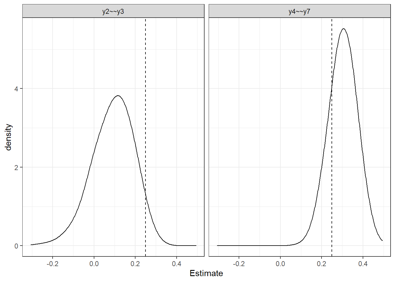
mean(sim.res[,1] > 0.25)[1] 0.027mean(sim.res[,2] > 0.25)[1] 0.791Laplace Approximation
wd <- getwd()
source(paste0(wd, "/code/utility_functions.R"))
  |
  |                                                                      |   0%
source(paste0(wd, "/code/laplace_functions.R"))
# specify population model
population.model <- '
f1 =~ 0.8*y1 + 0.8*y2 + 0.8*y3 + 0.8*y4
f2 =~ 0.8*y5 + 0.8*y6 + 0.8*y7 + 0.8*y8
f3 =~ 0.8*y9 + 0.8*y10 + 0.8*y11 + 0.8*y12
# Factor (co)variances
f1 ~~ 1*f1 + 0.3*f2 + 0.1*f3
f2 ~~ 1*f2 + 0.2*f3
f3 ~~ 1*f3
# residual covariances
y4 ~~ 0.3*y7
y2 ~~ 0.1*y3
'
# generate data
myData <- simulateData(population.model, sample.nobs=300L)
# fit model
myModel <- '
f1 =~ y1 + y2 + y3 + y4
f2 =~ y5 + y6 + y7 + y8
f3 =~ y9 + y10 + y11 + y12
# Factor covariances
f1 ~~ f2 + f3
f2 ~~ f3
'
fit <- cfa(myModel, data=myData)
summary(fit, standardized=T)lavaan 0.6-7 ended normally after 35 iterations
Estimator ML
Optimization method NLMINB
Number of free parameters 27
Number of observations 300
Model Test User Model:
Test statistic 64.649
Degrees of freedom 51
P-value (Chi-square) 0.095
Parameter Estimates:
Standard errors Standard
Information Expected
Information saturated (h1) model Structured
Latent Variables:
Estimate Std.Err z-value P(>|z|) Std.lv Std.all
f1 =~
y1 1.000 0.751 0.609
y2 1.181 0.154 7.647 0.000 0.887 0.660
y3 1.191 0.154 7.752 0.000 0.895 0.690
y4 0.897 0.131 6.851 0.000 0.674 0.544
f2 =~
y5 1.000 0.839 0.628
y6 0.952 0.122 7.825 0.000 0.798 0.655
y7 1.059 0.134 7.931 0.000 0.888 0.679
y8 0.858 0.119 7.195 0.000 0.720 0.567
f3 =~
y9 1.000 0.782 0.620
y10 1.043 0.138 7.546 0.000 0.816 0.635
y11 1.055 0.137 7.684 0.000 0.825 0.662
y12 0.999 0.135 7.412 0.000 0.782 0.613
Covariances:
Estimate Std.Err z-value P(>|z|) Std.lv Std.all
f1 ~~
f2 0.171 0.055 3.124 0.002 0.271 0.271
f3 0.085 0.048 1.770 0.077 0.144 0.144
f2 ~~
f3 0.114 0.054 2.110 0.035 0.173 0.173
Variances:
Estimate Std.Err z-value P(>|z|) Std.lv Std.all
.y1 0.959 0.101 9.509 0.000 0.959 0.630
.y2 1.019 0.118 8.613 0.000 1.019 0.564
.y3 0.882 0.111 7.985 0.000 0.882 0.524
.y4 1.080 0.105 10.316 0.000 1.080 0.704
.y5 1.081 0.116 9.276 0.000 1.081 0.606
.y6 0.846 0.096 8.794 0.000 0.846 0.570
.y7 0.922 0.111 8.324 0.000 0.922 0.539
.y8 1.094 0.108 10.111 0.000 1.094 0.678
.y9 0.982 0.105 9.312 0.000 0.982 0.616
.y10 0.989 0.109 9.064 0.000 0.989 0.597
.y11 0.872 0.102 8.550 0.000 0.872 0.561
.y12 1.016 0.108 9.415 0.000 1.016 0.624
f1 0.564 0.116 4.878 0.000 1.000 1.000
f2 0.704 0.139 5.075 0.000 1.000 1.000
f3 0.612 0.123 4.963 0.000 1.000 1.000lfit <- laplace_local_fit(
fit, data=myData, cut.load = 0.32, cut.cov = 0.25,
standardize = T, pb = F,
opt=list(scale.cov=1, no.samples=10000))library(kableExtra)
kable(lfit$Summary, format="html", digits=3) %>%
kable_styling(full_width = T) %>%
scroll_box(width="100%", height = "500px")| Parameter | Pr(|theta|>cutoff) | mean | sd | p0.025 | p0.25 | p0.5 | p0.75 | p0.975 |
|---|---|---|---|---|---|---|---|---|
| y7~~y4 | 0.823 | 0.307 | 0.062 | 0.185 | 0.266 | 0.308 | 0.350 | 0.429 |
| y11~~y8 | 0.071 | -0.150 | 0.068 | -0.282 | -0.196 | -0.151 | -0.105 | -0.016 |
| y7~~y3 | 0.046 | -0.123 | 0.075 | -0.268 | -0.174 | -0.123 | -0.071 | 0.022 |
| y11~~y1 | 0.043 | 0.131 | 0.069 | -0.001 | 0.084 | 0.130 | 0.179 | 0.267 |
| y5~~y4 | 0.024 | -0.117 | 0.067 | -0.248 | -0.162 | -0.117 | -0.071 | 0.012 |
| y4~~y3 | 0.022 | -0.104 | 0.073 | -0.246 | -0.155 | -0.104 | -0.055 | 0.040 |
| f2=~y4 | 0.021 | 0.157 | 0.079 | 0.004 | 0.103 | 0.157 | 0.211 | 0.314 |
| y5~~y1 | 0.019 | -0.109 | 0.068 | -0.243 | -0.154 | -0.109 | -0.062 | 0.024 |
| y12~~y1 | 0.019 | -0.113 | 0.068 | -0.244 | -0.159 | -0.113 | -0.068 | 0.021 |
| y10~~y8 | 0.018 | 0.111 | 0.067 | -0.020 | 0.066 | 0.111 | 0.156 | 0.242 |
| y8~~y4 | 0.015 | -0.115 | 0.064 | -0.239 | -0.158 | -0.115 | -0.072 | 0.009 |
| y5~~y2 | 0.015 | 0.101 | 0.069 | -0.036 | 0.054 | 0.101 | 0.148 | 0.237 |
| y2~~y1 | 0.012 | -0.088 | 0.073 | -0.230 | -0.138 | -0.088 | -0.039 | 0.056 |
| y7~~y2 | 0.011 | -0.078 | 0.074 | -0.223 | -0.127 | -0.078 | -0.029 | 0.068 |
| y10~~y7 | 0.010 | 0.082 | 0.072 | -0.058 | 0.033 | 0.082 | 0.131 | 0.223 |
| y7~~y6 | 0.010 | -0.074 | 0.076 | -0.222 | -0.126 | -0.075 | -0.023 | 0.076 |
| y12~~y3 | 0.009 | 0.084 | 0.072 | -0.060 | 0.036 | 0.085 | 0.132 | 0.224 |
| y10~~y5 | 0.008 | -0.089 | 0.069 | -0.225 | -0.136 | -0.089 | -0.042 | 0.045 |
| y6~~y1 | 0.008 | -0.078 | 0.070 | -0.216 | -0.124 | -0.078 | -0.030 | 0.059 |
| y8~~y1 | 0.007 | 0.092 | 0.066 | -0.033 | 0.047 | 0.092 | 0.138 | 0.221 |
| y10~~y3 | 0.007 | -0.073 | 0.072 | -0.212 | -0.121 | -0.073 | -0.024 | 0.071 |
| y12~~y6 | 0.006 | -0.077 | 0.069 | -0.217 | -0.123 | -0.077 | -0.030 | 0.056 |
| y12~~y4 | 0.006 | -0.082 | 0.066 | -0.210 | -0.126 | -0.082 | -0.037 | 0.047 |
| y11~~y6 | 0.006 | 0.071 | 0.072 | -0.069 | 0.023 | 0.071 | 0.121 | 0.213 |
| f1=~y7 | 0.004 | 0.082 | 0.087 | -0.085 | 0.024 | 0.082 | 0.140 | 0.255 |
| f3=~y7 | 0.004 | 0.087 | 0.085 | -0.083 | 0.031 | 0.087 | 0.143 | 0.254 |
| y9~~y3 | 0.004 | -0.056 | 0.072 | -0.197 | -0.105 | -0.056 | -0.006 | 0.087 |
| f2=~y10 | 0.003 | 0.098 | 0.080 | -0.060 | 0.045 | 0.098 | 0.153 | 0.257 |
| y11~~y2 | 0.003 | -0.050 | 0.072 | -0.193 | -0.100 | -0.051 | -0.002 | 0.092 |
| f2=~y3 | 0.003 | -0.096 | 0.081 | -0.255 | -0.151 | -0.095 | -0.041 | 0.060 |
| y10~~y4 | 0.003 | 0.064 | 0.067 | -0.071 | 0.019 | 0.065 | 0.109 | 0.195 |
| y10~~y9 | 0.003 | -0.052 | 0.071 | -0.190 | -0.100 | -0.052 | -0.004 | 0.088 |
| f1=~y11 | 0.002 | 0.083 | 0.084 | -0.084 | 0.027 | 0.084 | 0.139 | 0.247 |
| y5~~y3 | 0.002 | 0.041 | 0.072 | -0.100 | -0.007 | 0.041 | 0.090 | 0.181 |
| f2=~y12 | 0.002 | -0.091 | 0.080 | -0.247 | -0.145 | -0.092 | -0.037 | 0.064 |
| y3~~y2 | 0.002 | 0.060 | 0.067 | -0.073 | 0.015 | 0.060 | 0.106 | 0.189 |
| y9~~y2 | 0.002 | 0.050 | 0.071 | -0.091 | 0.002 | 0.049 | 0.097 | 0.191 |
| y12~~y2 | 0.002 | 0.043 | 0.070 | -0.095 | -0.005 | 0.042 | 0.090 | 0.181 |
| y8~~y5 | 0.002 | -0.053 | 0.069 | -0.188 | -0.099 | -0.052 | -0.007 | 0.083 |
| y4~~y1 | 0.002 | 0.068 | 0.063 | -0.057 | 0.026 | 0.068 | 0.110 | 0.190 |
| f3=~y5 | 0.002 | -0.071 | 0.086 | -0.239 | -0.130 | -0.071 | -0.013 | 0.095 |
| y12~~y11 | 0.002 | -0.042 | 0.072 | -0.183 | -0.090 | -0.042 | 0.007 | 0.096 |
| y9~~y5 | 0.002 | 0.053 | 0.068 | -0.081 | 0.006 | 0.053 | 0.099 | 0.186 |
| y6~~y4 | 0.001 | 0.055 | 0.067 | -0.078 | 0.010 | 0.055 | 0.099 | 0.187 |
| y11~~y5 | 0.001 | -0.036 | 0.070 | -0.173 | -0.083 | -0.036 | 0.012 | 0.099 |
| f2=~y1 | 0.001 | -0.080 | 0.077 | -0.233 | -0.132 | -0.080 | -0.028 | 0.072 |
| y11~~y3 | 0.001 | 0.002 | 0.075 | -0.147 | -0.048 | 0.001 | 0.053 | 0.148 |
| f1=~y5 | 0.001 | -0.057 | 0.086 | -0.228 | -0.114 | -0.055 | 0.001 | 0.109 |
| y11~~y4 | 0.001 | 0.025 | 0.067 | -0.109 | -0.021 | 0.025 | 0.070 | 0.157 |
| y6~~y5 | 0.001 | 0.046 | 0.066 | -0.084 | 0.001 | 0.046 | 0.092 | 0.174 |
| y11~~y7 | 0.001 | 0.030 | 0.073 | -0.112 | -0.019 | 0.030 | 0.080 | 0.169 |
| y12~~y10 | 0.001 | 0.046 | 0.066 | -0.081 | 0.002 | 0.046 | 0.090 | 0.177 |
| y3~~y1 | 0.001 | 0.046 | 0.068 | -0.087 | 0.000 | 0.047 | 0.090 | 0.177 |
| y8~~y3 | 0.001 | -0.020 | 0.070 | -0.157 | -0.067 | -0.020 | 0.028 | 0.117 |
| f1=~y12 | 0.001 | -0.067 | 0.084 | -0.232 | -0.123 | -0.067 | -0.011 | 0.099 |
| f3=~y3 | 0.001 | -0.054 | 0.085 | -0.219 | -0.112 | -0.054 | 0.003 | 0.112 |
| f3=~y2 | 0.001 | 0.039 | 0.087 | -0.128 | -0.019 | 0.040 | 0.097 | 0.210 |
| f3=~y8 | 0.001 | -0.044 | 0.084 | -0.208 | -0.099 | -0.043 | 0.013 | 0.117 |
| y9~~y1 | 0.001 | -0.019 | 0.069 | -0.156 | -0.065 | -0.018 | 0.029 | 0.114 |
| y10~~y1 | 0.001 | -0.033 | 0.069 | -0.166 | -0.081 | -0.033 | 0.013 | 0.104 |
| y10~~y2 | 0.001 | -0.005 | 0.072 | -0.146 | -0.053 | -0.005 | 0.042 | 0.135 |
| y12~~y7 | 0.001 | -0.023 | 0.072 | -0.165 | -0.072 | -0.023 | 0.025 | 0.116 |
| y8~~y6 | 0.001 | 0.037 | 0.064 | -0.091 | -0.007 | 0.037 | 0.081 | 0.165 |
| y10~~y6 | 0.001 | 0.016 | 0.071 | -0.121 | -0.032 | 0.015 | 0.065 | 0.156 |
| f3=~y4 | 0.000 | 0.067 | 0.083 | -0.094 | 0.010 | 0.066 | 0.123 | 0.231 |
| y7~~y1 | 0.000 | 0.018 | 0.071 | -0.124 | -0.029 | 0.018 | 0.066 | 0.159 |
| y9~~y4 | 0.000 | 0.029 | 0.067 | -0.103 | -0.015 | 0.029 | 0.074 | 0.161 |
| f1=~y10 | 0.000 | -0.032 | 0.086 | -0.200 | -0.090 | -0.033 | 0.026 | 0.136 |
| y6~~y2 | 0.000 | 0.010 | 0.071 | -0.127 | -0.039 | 0.010 | 0.059 | 0.154 |
| y8~~y2 | 0.000 | 0.013 | 0.069 | -0.121 | -0.033 | 0.014 | 0.059 | 0.148 |
| y6~~y3 | 0.000 | -0.002 | 0.073 | -0.146 | -0.051 | -0.002 | 0.048 | 0.140 |
| y9~~y7 | 0.000 | -0.008 | 0.071 | -0.148 | -0.055 | -0.008 | 0.040 | 0.133 |
| y11~~y9 | 0.000 | 0.036 | 0.067 | -0.094 | -0.010 | 0.035 | 0.080 | 0.170 |
| y12~~y9 | 0.000 | 0.007 | 0.067 | -0.125 | -0.038 | 0.007 | 0.053 | 0.139 |
| y11~~y10 | 0.000 | -0.008 | 0.070 | -0.142 | -0.054 | -0.007 | 0.039 | 0.130 |
| f2=~y2 | 0.000 | 0.044 | 0.082 | -0.117 | -0.013 | 0.043 | 0.100 | 0.206 |
| f3=~y1 | 0.000 | -0.035 | 0.083 | -0.196 | -0.090 | -0.035 | 0.022 | 0.127 |
| y7~~y5 | 0.000 | 0.018 | 0.068 | -0.115 | -0.029 | 0.017 | 0.063 | 0.151 |
| y8~~y7 | 0.000 | 0.023 | 0.067 | -0.109 | -0.022 | 0.024 | 0.068 | 0.155 |
| y9~~y8 | 0.000 | -0.014 | 0.068 | -0.144 | -0.061 | -0.015 | 0.032 | 0.121 |
| f1=~y6 | 0.000 | -0.018 | 0.083 | -0.177 | -0.073 | -0.018 | 0.038 | 0.146 |
| y9~~y6 | 0.000 | -0.008 | 0.071 | -0.147 | -0.056 | -0.008 | 0.040 | 0.132 |
| y4~~y2 | 0.000 | -0.011 | 0.067 | -0.145 | -0.057 | -0.011 | 0.035 | 0.120 |
| y12~~y8 | 0.000 | 0.014 | 0.066 | -0.117 | -0.031 | 0.014 | 0.058 | 0.142 |
| f1=~y8 | 0.000 | -0.017 | 0.086 | -0.184 | -0.075 | -0.017 | 0.040 | 0.150 |
| f1=~y9 | 0.000 | 0.006 | 0.085 | -0.165 | -0.050 | 0.007 | 0.063 | 0.171 |
| f2=~y11 | 0.000 | -0.039 | 0.079 | -0.193 | -0.093 | -0.038 | 0.016 | 0.115 |
| f3=~y6 | 0.000 | 0.005 | 0.081 | -0.154 | -0.050 | 0.004 | 0.060 | 0.164 |
| y12~~y5 | 0.000 | 0.008 | 0.069 | -0.128 | -0.037 | 0.008 | 0.055 | 0.143 |
| f2=~y9 | 0.000 | 0.023 | 0.078 | -0.132 | -0.030 | 0.023 | 0.075 | 0.176 |
Sampling Distributions
# transform
plot_dat_laplace <- lfit$`All Results` %>%
  pivot_longer(
    cols=everything(),
    names_to = "Parameter",
    values_to = "Estimate"
  )

plot_dat_laplace <- filter(plot_dat_laplace,
                           Parameter %in% c("y3~~y2", "y7~~y4")) %>%
  mutate(V = ifelse(Parameter %like% "=~", 0.32, 0.25),
         Parameter = ifelse(Parameter == "y3~~y2",
                            "cov(y[2], y[3])", "cov(y[4], y[7])"))


plot_dat_emp <- sim.res %>%
  pivot_longer(
    cols=everything(),
    names_to = "Parameter",
    values_to = "Estimate"
  ) %>%
  mutate(V = ifelse(Parameter %like% "=~", 0.32, 0.25),
         Parameter = ifelse(Parameter == "y2~~y3",
                            "cov(y[2], y[3])", "cov(y[4], y[7])"))

lty <- c("True" = 1, "Laplace" = 2)

p <- ggplot()+
  geom_density(data=plot_dat_emp, adjust = 2,
               aes(x=Estimate, linetype="True"))+
  geom_density(data=plot_dat_laplace, adjust = 2,
               aes(x=Estimate, linetype="Laplace"))+
  #geom_vline(xintercept = 0.25, linetype="dotted")+
  scale_linetype_manual(values = lty, name=NULL)+
  facet_wrap(.~Parameter, labeller = label_parsed)+
  theme_bw() +
  theme(panel.grid = element_blank(),
        strip.background = element_blank(),
        legend.position = "bottom",
        text=element_text(size=13))
p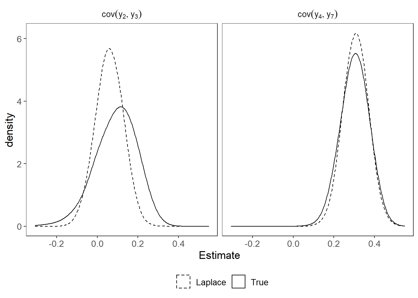
ggsave("manuscript/fig/sampling_dist.pdf", p, units="in", width=7, height=3.5)
sessionInfo()R version 4.0.2 (2020-06-22)
Platform: x86_64-w64-mingw32/x64 (64-bit)
Running under: Windows 10 x64 (build 18362)
Matrix products: default
Random number generation:
RNG: L'Ecuyer-CMRG
Normal: Inversion
Sample: Rejection
locale:
[1] LC_COLLATE=English_United States.1252
[2] LC_CTYPE=English_United States.1252
[3] LC_MONETARY=English_United States.1252
[4] LC_NUMERIC=C
[5] LC_TIME=English_United States.1252
attached base packages:
[1] tcltk stats graphics grDevices utils datasets methods
[8] base
other attached packages:
[1] kableExtra_1.1.0 data.table_1.13.0 mvtnorm_1.1-1 coda_0.19-3
[5] simsem_0.5-15 lavaan_0.6-7 ggplot2_3.3.2 dplyr_1.0.1
[9] tidyr_1.1.1 xtable_1.8-4 workflowr_1.6.2
loaded via a namespace (and not attached):
[1] tidyselect_1.1.0 xfun_0.16 purrr_0.3.4 lattice_0.20-41
[5] colorspace_1.4-1 vctrs_0.3.2 generics_0.0.2 viridisLite_0.3.0
[9] htmltools_0.5.0 stats4_4.0.2 yaml_2.2.1 rlang_0.4.7
[13] later_1.1.0.1 pillar_1.4.6 glue_1.4.1 withr_2.2.0
[17] lifecycle_0.2.0 stringr_1.4.0 munsell_0.5.0 gtable_0.3.0
[21] rvest_0.3.6 evaluate_0.14 labeling_0.3 knitr_1.29
[25] httpuv_1.5.4 parallel_4.0.2 highr_0.8 Rcpp_1.0.5
[29] readr_1.3.1 promises_1.1.1 backports_1.1.7 scales_1.1.1
[33] webshot_0.5.2 tmvnsim_1.0-2 farver_2.0.3 fs_1.5.0
[37] mnormt_2.0.1 hms_0.5.3 digest_0.6.25 stringi_1.4.6
[41] grid_4.0.2 rprojroot_1.3-2 tools_4.0.2 magrittr_1.5
[45] tibble_3.0.3 crayon_1.3.4 whisker_0.4 pbivnorm_0.6.0
[49] pkgconfig_2.0.3 ellipsis_0.3.1 MASS_7.3-51.6 xml2_1.3.2
[53] httr_1.4.2 rmarkdown_2.3 rstudioapi_0.11 R6_2.4.1
[57] git2r_0.27.1 compiler_4.0.2