

Refer to the readme file for a quick start with examples and use cases.
A few illustrations of the basic built-in plotting functions


Construct a prospect in a decision-making problem.
trials - an integer defining the number of rounds in the choice problem.
fun - a functions that returns numeric outcomes (or an outcome, if oneOutcomePerRun is True).
oneOutcomePerRun - Boolean, if True - when generating the outcomes, the function runs trials number of times. If False, the function should return an array of outcomes in the size of trials.
*args, **kwargs - Arguments to be passed to fun.
Example:
Use NumPy's random.choice to generate 100 outcomes: each outcome is 3 with
probability 0.45 and zero otherwise.
A=Prospect(100,np.random.choice,False,[3,0],100,True,[0.45,0.55])
Generate new outcomes (stored internally).
Calculate the expected value, based on EVsims simulations.
Plot the outcomes based on nsim simulations.
If blocks is None - plot all trials; Else, aggregate over blocks
blocks.
Returns: fig, ax
A>B - the proportion of times the outcomes of A are greater than the outcomes of B, based on 1000 simulations (works with '<' as well).
A==B - the proportion of times the outcomes of A equal the outcomes of B, based on 1000 simulations.
Construct a model object which includes the environment (the decision-making problem formulated in prospects, the behavior of the agents and their parameters), the number of simulations required for making predictions, and whether the decision-task provides full or partial feedback.
parameters - a dictionary (preferred) or a list of parameters' values. For instance {'Lambda': 0.1}. The value could be None (if no predictions are needed) or numeric.
prospects - a list of pre-defined Prospect objects. For example [StatusQuo, RiskyOption, Neutral].
nsim - an integer representing the number of simulations needed in every run of Predict.
FullFeedback - Boolean. Sets the decision-problem feedback scope (False == feedback for the chosen prospect only; True == feedback for all prospects). Note that not all models support partial feedback, hence the default True value.
Specific types of models may add additional arguments prior to parameters, refer to the documentation of the specific model you are using.
Store the observed choices internally (mandatory for plotting model's fit or estimating the model's parameters).
oc - an array with a shape of trials x prospects (i.e., each prospect is a column). Values should range from 0 to 1, inclusive.
Returns the currently stored predictions. Could be None if no predictions were made (i.e., Model.Predict() was not run, and the model was not fitted to data).
Returns an array with a shape of trials x prospects.
Save currently stored predictions into a csv file.
fname - file name to save the data to (note: will override the file).
Returns the value of the loss function using the stored parameters, predictions, and observations.
loss - the loss function. Either MSE (a.k.a MSD) or LL (minus log-likelihood).
scope - the scope of the loss calculation. If prospectwise (or
pw), will use the aggregated choices (i.e., mean choice rates over
trials).
If bitwise (or bw) will use the trial level data.
Returns a float.
Plots the stored predicted values in trials or blocks. Returns matplotlib objects (fig, axes) for further processing of the figure.
blocks - if None (default), will plot the predictions over trials. If an integer, will split the data into blocks of size trials/blocks.
**args - pass keyword arguments into pyplot.plot.
Returns: Fig, Axes.
Plots the stored observed values in trials or blocks. Returns matplotlib objects (fig, axes) for further processing of the figure.
blocks - if None (default), will plot the observations over trials. If an integer, will split the data into blocks of size trials/blocks.
**args - pass keyword arguments into pyplot.plot.
Returns: Fig, Axes.
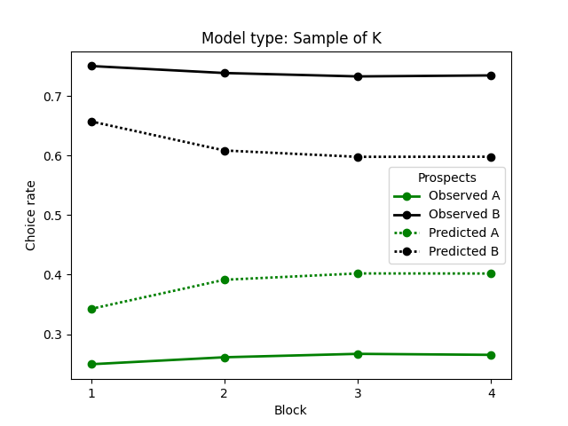
Plots both observed and predicted values in trials or blocks. Returns matplotlib objects (fig, axes) for further processing of the figure.
blocks - if None (default), will plot the values over trials. If an integer, will split the data into blocks of size trials/blocks.
**args - pass keyword arguments into pyplot.plot.
Returns: Fig, Axes.
Similar to Model.loss, only that parameters are passed and
Model.Predict() is run before returning the loss.
Useful for using external optimization algorithms that pass parameters as
arguments and expect a loss value in return.
parameters - a dictionary or a list of parameters' values. For
instance {'Lambda': 0.1}. The value could be None (if no predictions are
needed) or numeric.
The list should be ordered similarly to the order once the model was
initiated.
*args- arguments to be passed to the loss function.
If two arguments are passed, they represent the loss and scope
parameters (see Model.loss).
If three arguments are passed, the first represents the reGenerate
argument (boolean) in Model.Predict, and the other two the loss and
scope parameters (see Model.loss).
**kwargs - keyword arguments to be passed to the loss function.
Example: Model.CalcLoss({'Alpha':2.3}, 'MSE', 'pw').
Returns a float representing the loss function at the particular point in parameters.
An exhaustive grid search (defined by the user). Returns the best set of
parameters that were searched.
Slow, but works with all types of models. Note that multiprocessing is
supported for reducing run time.
pars_dicts - a list of dictionaries, where each dictionary contains values for all parameters in the model. For example:
[{'Alpha':0.1, 'Lambda':0.1}, {'Alpha':0.1, 'Lambda':0.2}, {'Alpha':0.1, 'Lambda':0.3}, {'Alpha':0.2, 'Lambda':0.1},....]
pb - show a progress bar (True/False).
*args - arguments to be passed to CalcLoss.
**kwargs - keyword arguments to be passed to CalcLoss.
Returns a dictionary of results, with the following keys:
bestp - a dictionary with the best set of parameters found.
losses - an array of the loss value for each set of parameters.
minloss - the value of the min loss.
parameters_checked - equals pars_dict
Tip: use makeGrid to create pars_dicts.
Example:
pspace=makeGrid({'Alpha':range(0,101), 'Lambda':np.arange(0,1,0.001})
results=myModel.OptimizeBF(pspace, True, 'MSE', 'pw')
This function is the core behavioral model that generates predictions according to the given prospects.
It accepts reGenerate as an input, which determines if the outcomes of each prospect are re-generated in each simulation.
Returns an array of predictions with a shape of trials x prospects.These predictions are also internally stored for further usage (e.g., plotting or fitting).
Configure multiprocessing. Multiprocessing allows faster code execution by utilizing more than one CPU at the time.
Example:
Model.mp=6 #use six CPUs.
Model.mp=1 #Disable multiprocessing. Any number smaller than 2 will have the same effect of disabling multiprocessing.
Note (1): If the number of chosen CPUs is smaller than the number of available CPUs, all CPUs will be used.
Note (2): Currently multiprocessing affects OptimizeBF method only.
This object allows fitting over multiple models and observations, for examples when agents complete more than one decision-making problem.
models - a list of models. All models should be of the same type because the same set of parameters is passed to every model in the list.
obs_choices - a list of matrices where each matrix is in the shape of trials x prospects, containing the observed choices.
See Model.CalcLoss for the description of arguments.
Fit over all models. For a detailed description of the arguments and returned values, see Model.OptimizeBF.
Make a grid for grid search (OptimizeBF).
pars_dict - a dictionary of parameters with iterables.
Returns: a list of dictionaries with a combination of all parameters' values sets.
Example 1:
grid=makeGrid({'Alpha':range(1,11)})
print(grid)
Example 2:
grid=makeGrid({'Alpha':[1,2,3],'Lambda':[0.1,0.5,0.9]})
print(grid)
Example 3:
grid=makeGrid({'Alpha':np.arange(1,20,6),'Lambda':np.arange(0,1,0.3)})
print(grid)
Save estimation results to a csv file.
res - a results dictionary generated by OptimizeBF.
fname - the name of the file to be saved (note: overrides an existing file).
**kwargs - optional keyword arguments to be passed to Pandas.to_csv
Plot the results of a results dictionary (generated by OptimizeBF)
In case of a one-parameter model, will plot a 2D figure.
In case of a two-parameter model, will plot a 3D figure.
In other cases, the X axis will show the iteration number (less useful).
Returns: fig, ax (one or two parameters) or fig, ax, surf (3 parameters).
The following is a template that one could use:
class yourModeName(Model):
def __init__(self,*args):
Model.__init__(self,*args)
self.name="Give your model a
name"
def Predict(self, reGenerate=True):
if type(self.parameters)==dict:
self._x=self.parameters['X'] # Read parameters (dict style)
self._y=self.parameters['Y']
# change the
naming of the parameters add more if needed
elif
type(self.parameters)==list:
self._x=self.parameters[0] # Read parameters (list style)
self._y=self.parameters[1]
# add more if
needed
else:
raise
Exception("Parameters should be a list or a
dictionary")
grand_choices=np.zeros((self.nsim,self._trials_,self._Num_of_prospects_))
#this would be an array of predicted choices
for s in range(self.nsim):
if
reGenerate:
for p in self.prospects:
p.Generate()
data=np.vstack([x.outcomes for x in self.prospects]).transpose() #This is
an array containing the outcomes from all prospects (shaped trials x
prospects)
for i in range(self._trials_): # In this template we iterate over trials
if i==0: # Assume random choice in the first trial
choice=np.random.choice(self._Num_of_prospects_)
grand_choices[s,i,choice]=1
else:
# This is the main "brain" of your model
# Stating what happens in every trial
# (after the first random choice)
# i is the trial index (starting
from 0)
# s is the simulation index.
# grand_choices is the matrix where
you store choices
# You should set the chosen choice
to 1 in each trial (or a value between 0 to 1 if your model is built this
way).
# For instance, if s=5, i=10, and
c=2,
# grand_choices[s,i,c]=1 means that
in the 6th
# simulation (indexing in Python
start from 0),
# on the 11th trial, the 3rd choice
is chosen.
# Row 11 in the 6th simulation will
look like that:
# 0 0 1 (assuming there are three
prospects).
self._pred_choices_=np.mean(grand_choices,axis=0) # Average accross
simulations,
#Store internally in
self._pred_choices_
return self._pred_choices_ #
Return the predicted choices
```
Thus, the minimal steps for creating your own model involve
setting up a name, the parameters, and writing the main algorithm (the
"brain" of your model).
Use all available historical feedback in each trial.
A K sized sample is drawn with replacement in each trial (after a first
random choice), and a prospect is chosen according to the best average of
the sample.
In each simulation a new K is drawn from a uniform distribution between 1
to Kappa.
Additionally, if kappa_or_less==True, in each trial the sample size is
drawn from 1 to K (thus, the sample size changes from trial to trial).
Arguments: kappa_or_less (Boolean), see explanation above.
Parameters: Kappa (integer, 1 to the number of trials).
Sample of K is essentially the Naive Sampler, with kappa_or_less set to False.
Parameters: Kappa (integer, 1 to the number of trials).
Two-stage Naive Sampler. In the first stage, decide between the risky
choices. In the second stage, decide between
the chosen risky choice and the rest of the choices.
Special methods: Optimize_Simplex