Travel time to major cities
Om Prakash Bhandari (Author), Johannes Schielein (Review)
6/4/2021
Last updated: 2021-09-15
Checks: 7 0
Knit directory: mapme.protectedareas/
This reproducible R Markdown analysis was created with workflowr (version 1.6.2). The Checks tab describes the reproducibility checks that were applied when the results were created. The Past versions tab lists the development history.
Great! Since the R Markdown file has been committed to the Git repository, you know the exact version of the code that produced these results.
Great job! The global environment was empty. Objects defined in the global environment can affect the analysis in your R Markdown file in unknown ways. For reproduciblity it’s best to always run the code in an empty environment.
The command set.seed(20210305) was run prior to running the code in the R Markdown file. Setting a seed ensures that any results that rely on randomness, e.g. subsampling or permutations, are reproducible.
Great job! Recording the operating system, R version, and package versions is critical for reproducibility.
Nice! There were no cached chunks for this analysis, so you can be confident that you successfully produced the results during this run.
Great job! Using relative paths to the files within your workflowr project makes it easier to run your code on other machines.
Great! You are using Git for version control. Tracking code development and connecting the code version to the results is critical for reproducibility.
The results in this page were generated with repository version 2fc3683. See the Past versions tab to see a history of the changes made to the R Markdown and HTML files.
Note that you need to be careful to ensure that all relevant files for the analysis have been committed to Git prior to generating the results (you can use wflow_publish or wflow_git_commit). workflowr only checks the R Markdown file, but you know if there are other scripts or data files that it depends on. Below is the status of the Git repository when the results were generated:
Ignored files:
    Ignored:    .RData
    Ignored:    .Rhistory
    Ignored:    .Rproj.user/
    Ignored:    data-raw/addons/docs/rest/
    Ignored:    data-raw/addons/etc/
    Ignored:    data-raw/addons/scripts/

Untracked files:
    Untracked:  .tmp/
Note that any generated files, e.g. HTML, png, CSS, etc., are not included in this status report because it is ok for generated content to have uncommitted changes.
These are the previous versions of the repository in which changes were made to the R Markdown (analysis/accessibility.rmd) and HTML (docs/accessibility.html) files. If you’ve configured a remote Git repository (see ?wflow_git_remote), click on the hyperlinks in the table below to view the files as they were in that past version.
| File | Version | Author | Date | Message |
|---|---|---|---|---|
| html | d1cfe2d | Johannes Schielein | 2021-09-15 | initial comit with sampling code |
| Rmd | b589068 | Ohm-Np | 2021-07-03 | update author names, urls & source code description |
| html | 1468f42 | Ohm-Np | 2021-07-03 | update html files |
| html | fa42f34 | Johannes Schielein | 2021-07-01 | Host with GitHub. |
| html | 8bd1321 | Johannes Schielein | 2021-06-30 | Host with GitLab. |
| html | 3a39ee3 | Johannes Schielein | 2021-06-30 | Host with GitHub. |
| html | ae67dca | Johannes Schielein | 2021-06-30 | Host with GitLab. |
| Rmd | a4ff10a | Om Bandhari | 2021-06-30 | update rmd analysis |
| html | 1a16e9c | Om Bandhari | 2021-06-30 | update html |
| html | e2e3cf5 | Om Bandhari | 2021-06-11 | updates accessibility files |
| Rmd | 9665e49 | Om Bandhari | 2021-06-11 | create accessibility rmarkdown |
# load required libraries
library("sf")
library("terra")
library("wdpar")
library("tidyverse")

starttime<-Sys.time() # mark the start time of this routine to calculate processing time at the end
Introduction
The term “accessibility” refers to the ability to reach promptly or to be able to attain something easily. Thus, accessibility is the ease with which larger cities can be reached from a certain location, in our case, from the protected areas. Accessibility is one of the most important factors to influence the likelihood of an area being exploited or converted for commercial purposes. Higher the accessibility to protected areas, higher the chances of anthropogenic disturbances to the ecosystem. So, it is of utmost importance to find out how much travel time could it take to reach the vicinity of a particular protected area.
For this analysis, we’ll look at a few protected areas and determine the minimum travel time to nearby cities, thus accessibility to the cities.
Datasource and Metadata Information
- Dataset: Travel Time to Cities and Ports 2015 (Weiß et al. (2018))
- Geographical Coverage: Global
- Spatial resolution: 1 kilometer
- Temporal Coverage: 2015
- Unit: minutes
- Data downloaded: 8th June, 2021
- Metadata Link
- Download Link
Processing Workflow
The purpose of this analysis is to compute minimum travel time from the protected area of interest to the nearby cities. For this, following processing routine is followed:
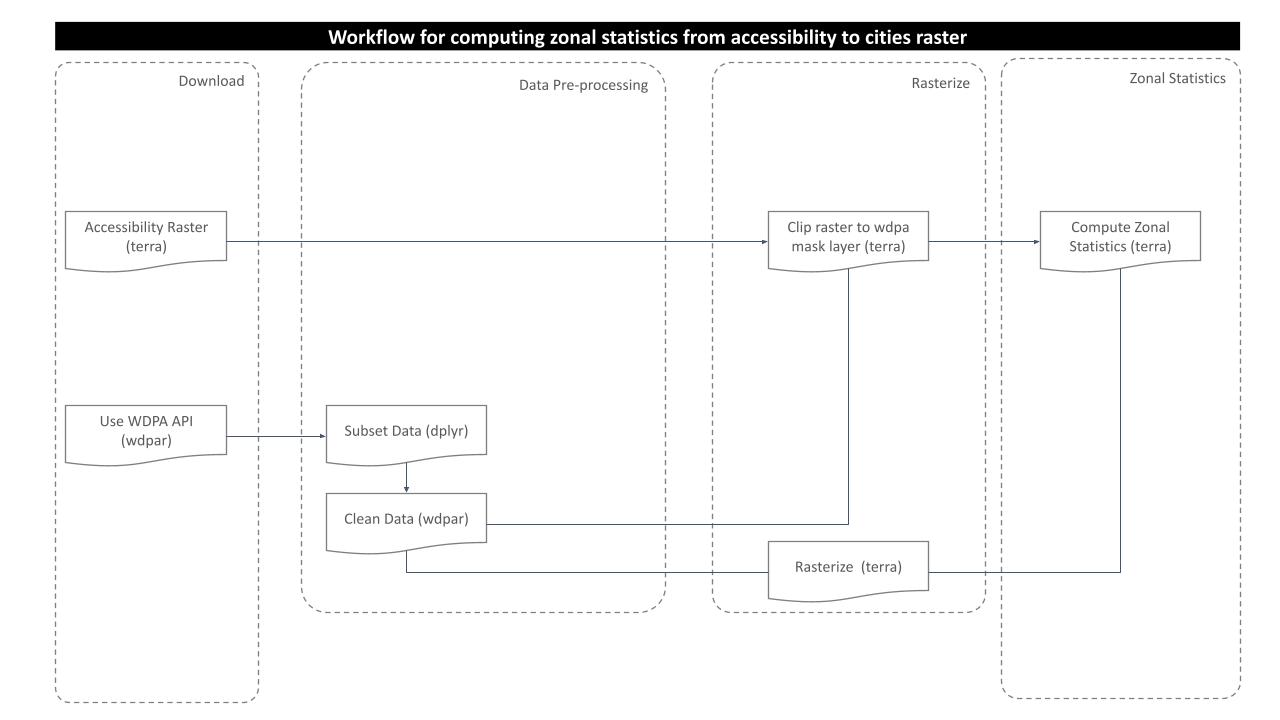
Download and Prepare WDPA Polygons
For this analysis, we would try to get the country level polygon data from wdpar package. wdpar is a library to interface to the World Database on Protected Areas (WDPA). The library is used to monitor the performance of existing PAs and determine priority areas for the establishment of new PAs. We will use Brazil - for other countries of your choice, simply provide the country name or the ISO name e.g. Gy for Guyana, COL for Colombia.
# fetch the raw data from wdpar of country
br_wdpa_raw <-
  wdpa_fetch("Brazil")
Since there are more than 3000 enlisted protected areas in Brazil, we want to compute zonal statistics only for the polygon data of: - Reserva Biologica Do Rio Trombetas - wdpaid 43, - Reserva Extrativista Rio Cajari - wdpaid 31776, and - Estacao Ecologica Do Jari - wdpaid 4891
For this, we have to subset the country level polygon data to the pa level.
# subset three wdpa polygons by their wdpa ids
br_wdpa_subset <-
  br_wdpa_raw%>%
  filter(WDPAID %in% c(43,4891,31776))
The next immediate step would be to clean the fetched raw data with the functionality provided with routines from the wdpar package. Cleaning is done by the package following this steps:
- exclude protected areas that are not yet implemented
- exclude protected areas with limited conservation value
- replace missing data codes (e.g. “0”) with missing data values (i.e. NA)
- replace protected areas represented as points with circular protected areas that correspond to their reported extent
- repair any topological issues with the geometries
# clean the data
br_wdpa_subset <- wdpa_clean(
  br_wdpa_subset,
  erase_overlaps = F
  )
# reproject to the WGS84
br_wdpa_subset <- st_transform(br_wdpa_subset,
                               "+proj=longlat +datum=WGS84 +no_defs")
# spatvector for terra compatibility
br_wdpa_subset_v <-
  vect(br_wdpa_subset)
# we can plot the data to see the three selected polygons
plot(br_wdpa_subset_v)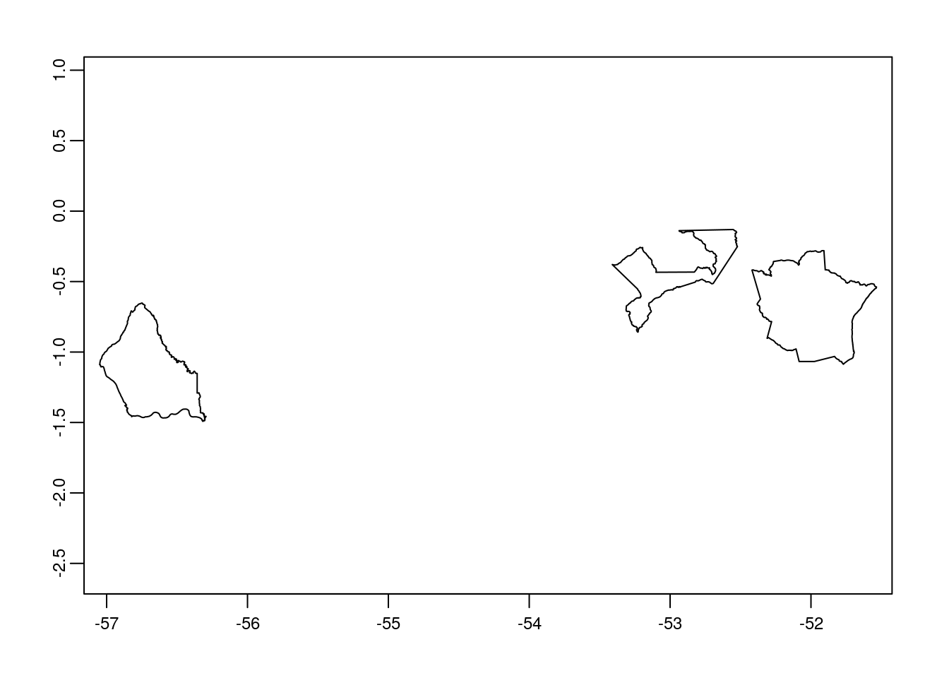
Prepare accessibility raster data
The raster datasets are available to download for 12 different layers for the year 2015, based on the different sets of urban areas defined by their population. Here, we are going to load the raster layer for the population range 50k to 100k using package terra.
# load accessibility raster
acc_rast <-
  rast("../../datalake/mapme.protectedareas/input/accessibility_to_cities/2015/acc_50k_100k.tif")
# view raster details
acc_rast
class : SpatRaster
dimensions : 17400, 43200, 1 (nrow, ncol, nlyr)
resolution : 0.008333333, 0.008333333 (x, y)
extent : -180, 180, -60, 85 (xmin, xmax, ymin, ymax)
coord. ref. : +proj=longlat +datum=WGS84 +no_defs
source : acc_50k_100k.tif
name : acc_50k_100k Crop the accessibility raster
As we completed raster and vector data preparation, the next step would be to clip the raster layer by the selected protected areas polygon both by its extent and mask layer. If we clip by extent, it does clipping the raster by its bounding box. However, using mask function returns the raster to defined vector polygon layer, which is a must for zonal statistics computation.
# crop raster by polygon
acc_rast_crop <-
        terra::crop(acc_rast,
                    br_wdpa_subset_v)
# plot the cropped raster layer
plot(acc_rast_crop)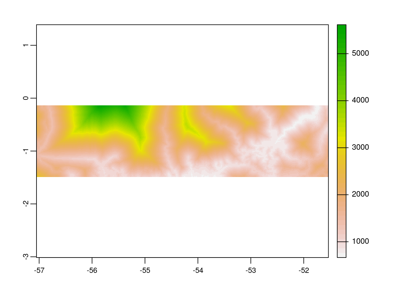
# mask the raster by polygon
acc_rast_mask <-
        terra::mask(acc_rast_crop,
                    br_wdpa_subset_v)
# plot the masked raster layer
plot(acc_rast_mask)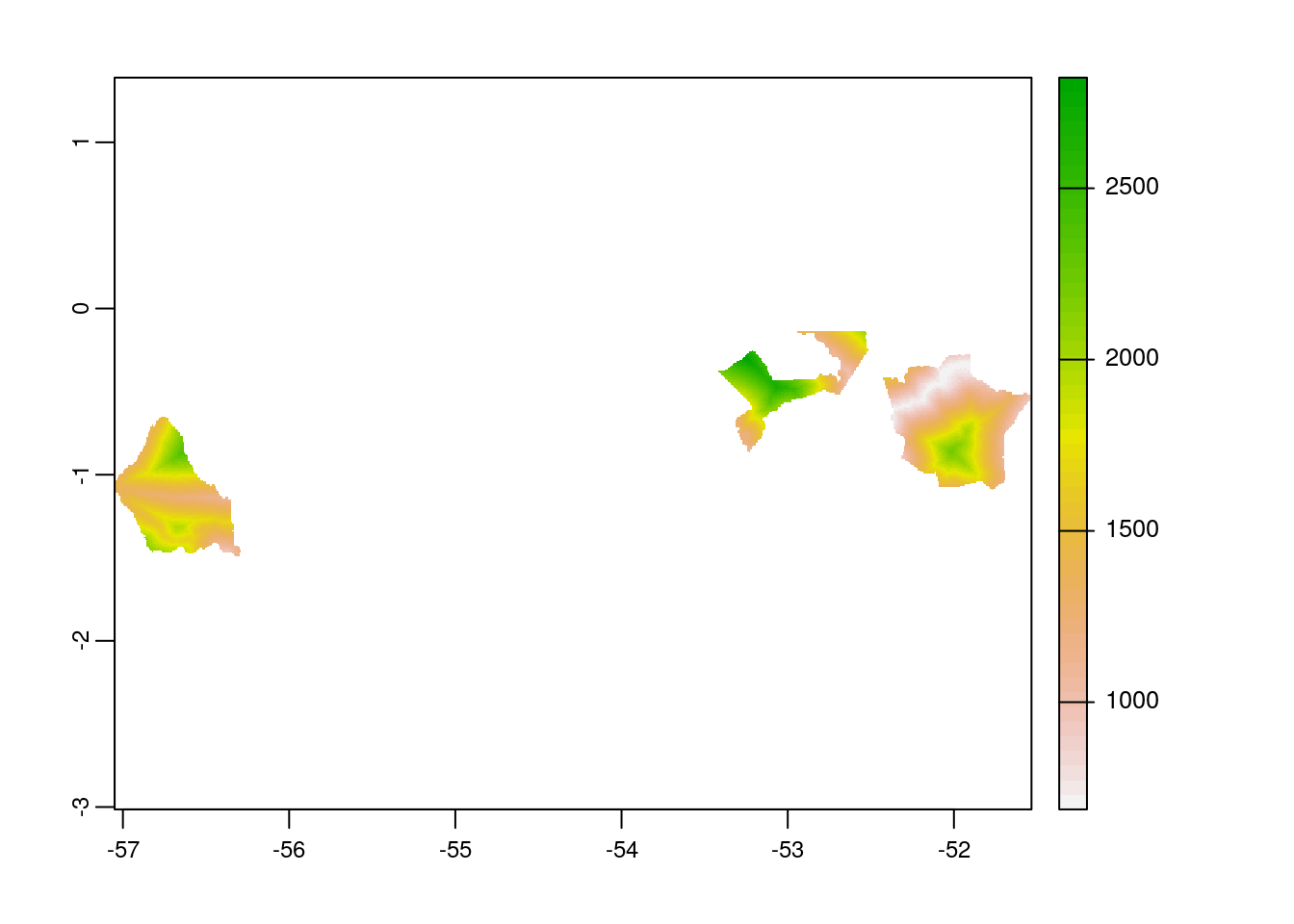
Rasterize the polygon layer
To compute the zonal statistics, it is necessary to rasterize the polygon layer. Doing so, values are transferred from the spatial objects to raster cells. We need to pass the extent layer and the mask layer to the rasterize function.
# rasterize the polygon
br_subset_rast <-terra::rasterize(br_wdpa_subset_v,
                                  acc_rast_mask,
                                  br_wdpa_subset_v$WDPAID)
# plot the rasterized polygon
plot(br_subset_rast)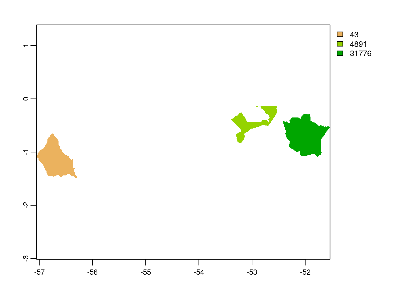
Compute Zonal Statistics - travel time to nearby cities
A zonal statistics operation is one that calculates statistics on cell values of a raster (a value raster) within the zones defined by another dataset [ArcGIS definition]. Here, we are interested on only to compute the minimum travel time to the cities, so, we would use function min for zonal operation.
# zonal stats
zstats <- terra::zonal(acc_rast_mask,
                       br_subset_rast,
                       fun='min',
                       na.rm=T)
# create dataframe to receive the result
df.zstats <- data.frame(WDPAID=NA,
                        travel_time_to_nearby_cities_min=NA)
# rename column to match with dataframe
colnames(zstats) <- colnames(df.zstats)
# view the data
rbind(df.zstats,zstats)[-1,]
WDPAID travel_time_to_nearby_cities_min
2 43 981
3 4891 979
4 31776 687From the zonal statistics result, we can see that to travel to the nearby cities from these regions, it takes more than 10 hours. Hence, we can say that these protected areas are not easily accessible.
In the end we are going to have a look how long the rendering of this file took to get an idea about the processing speed of this routine.
stoptime<-Sys.time()
print(starttime-stoptime)
Time difference of -4.251817 secsReferences
[1] Weiss, D. J., Nelson, A., Gibson, H. S., Temperley, W., Peedell, S., Lieber, A., … & Gething, P. W. (2018). A global map of travel time to cities to assess inequalities in accessibility in 2015. Nature, 553(7688), 333-336.
sessionInfo()R version 3.6.3 (2020-02-29)
Platform: x86_64-pc-linux-gnu (64-bit)
Running under: Ubuntu 18.04.5 LTS
Matrix products: default
BLAS: /usr/lib/x86_64-linux-gnu/blas/libblas.so.3.7.1
LAPACK: /usr/lib/x86_64-linux-gnu/lapack/liblapack.so.3.7.1
locale:
[1] LC_CTYPE=C.UTF-8 LC_NUMERIC=C LC_TIME=C.UTF-8
[4] LC_COLLATE=C.UTF-8 LC_MONETARY=C.UTF-8 LC_MESSAGES=C.UTF-8
[7] LC_PAPER=C.UTF-8 LC_NAME=C LC_ADDRESS=C
[10] LC_TELEPHONE=C LC_MEASUREMENT=C.UTF-8 LC_IDENTIFICATION=C
attached base packages:
[1] stats graphics grDevices utils datasets methods base
other attached packages:
[1] forcats_0.5.1 stringr_1.4.0 dplyr_1.0.6 purrr_0.3.4
[5] readr_1.4.0 tidyr_1.1.3 tibble_3.1.1 ggplot2_3.3.4
[9] tidyverse_1.3.1 wdpar_1.0.6 terra_1.2-15 sf_0.9-8
loaded via a namespace (and not attached):
[1] httr_1.4.2 jsonlite_1.7.2 modelr_0.1.8 assertthat_0.2.1
[5] countrycode_1.2.0 sp_1.4-5 cellranger_1.1.0 yaml_2.2.1
[9] pillar_1.6.0 backports_1.2.1 lattice_0.20-44 glue_1.4.2
[13] digest_0.6.27 promises_1.2.0.1 rvest_1.0.0 colorspace_2.0-1
[17] htmltools_0.5.1.1 httpuv_1.6.1 pkgconfig_2.0.3 broom_0.7.6
[21] raster_3.4-13 haven_2.3.1 scales_1.1.1 whisker_0.4
[25] later_1.2.0 git2r_0.28.0 proxy_0.4-26 generics_0.1.0
[29] ellipsis_0.3.2 withr_2.4.2 cli_2.5.0 magrittr_2.0.1
[33] crayon_1.4.1 readxl_1.3.1 evaluate_0.14 fs_1.5.0
[37] fansi_0.5.0 xml2_1.3.2 lwgeom_0.2-6 class_7.3-19
[41] tools_3.6.3 hms_1.0.0 lifecycle_1.0.0 munsell_0.5.0
[45] reprex_2.0.0 compiler_3.6.3 e1071_1.7-7 rlang_0.4.11
[49] classInt_0.4-3 units_0.7-1 grid_3.6.3 rstudioapi_0.13
[53] rappdirs_0.3.3 rmarkdown_2.6 gtable_0.3.0 codetools_0.2-18
[57] DBI_1.1.1 curl_4.3.2 R6_2.5.0 lubridate_1.7.10
[61] knitr_1.30 utf8_1.2.1 workflowr_1.6.2 rprojroot_2.0.2
[65] KernSmooth_2.23-20 stringi_1.6.2 Rcpp_1.0.7 vctrs_0.3.8
[69] dbplyr_2.1.1 tidyselect_1.1.1 xfun_0.24