Climatic variables - Precipitation and temperature
Om Prakash Bhandari (Author), Johannes Schielein (Review)
11/23/2021
Last updated: 2021-12-14
Checks: 6 1
Knit directory: mapme.protectedareas/
This reproducible R Markdown analysis was created with workflowr (version 1.6.2). The Checks tab describes the reproducibility checks that were applied when the results were created. The Past versions tab lists the development history.
The R Markdown is untracked by Git. To know which version of the R Markdown file created these results, you’ll want to first commit it to the Git repo. If you’re still working on the analysis, you can ignore this warning. When you’re finished, you can run wflow_publish to commit the R Markdown file and build the HTML.
Great job! The global environment was empty. Objects defined in the global environment can affect the analysis in your R Markdown file in unknown ways. For reproduciblity it’s best to always run the code in an empty environment.
The command set.seed(20210305) was run prior to running the code in the R Markdown file. Setting a seed ensures that any results that rely on randomness, e.g. subsampling or permutations, are reproducible.
Great job! Recording the operating system, R version, and package versions is critical for reproducibility.
Nice! There were no cached chunks for this analysis, so you can be confident that you successfully produced the results during this run.
Great job! Using relative paths to the files within your workflowr project makes it easier to run your code on other machines.
Great! You are using Git for version control. Tracking code development and connecting the code version to the results is critical for reproducibility.
The results in this page were generated with repository version 13c3cce. See the Past versions tab to see a history of the changes made to the R Markdown and HTML files.
Note that you need to be careful to ensure that all relevant files for the analysis have been committed to Git prior to generating the results (you can use wflow_publish or wflow_git_commit). workflowr only checks the R Markdown file, but you know if there are other scripts or data files that it depends on. Below is the status of the Git repository when the results were generated:
Ignored files:
    Ignored:    .Rproj.user/

Untracked files:
    Untracked:  analysis/climatic-variables.rmd

Unstaged changes:
    Modified:   analysis/index.Rmd
    Modified:   code/big_data_processing.R
    Modified:   code/development/download-scripts.R
Note that any generated files, e.g. HTML, png, CSS, etc., are not included in this status report because it is ok for generated content to have uncommitted changes.
There are no past versions. Publish this analysis with wflow_publish() to start tracking its development.
# load required libraries
library("sf")
library("terra")
library("wdpar")
library("tidyverse")

starttime <- Sys.time() # mark the start time of this routine to calculate processing time at the end
Introduction
Climate change is one of the hottest issues around the globe in the present context. Existence of flora and fauna has been affected thoroughly with the rise in temperature and infrequent rainfall happening throughout different forests ecosystem. In context of protected areas, it is even more important to see the pattern of temperature and rainfall not only to assess the change issues but also to get the idea on how diverse is the protected area in terms of weather and climate. So, here in this analysis, we are going to demonstrate how to process precipitation and temperature data and get the average temperature and precipitation values in our protected area polygons of interest.
Datasource and Metadata Information
- Dataset: Historical climate data (WorldClim) [1]
- Geographical Coverage: Global
- Spatial resolution: ~ 1 km
- Temporal Coverage: 1970-2000
- Unit: precipitation (mm) & temperature (°C)
- Data downloaded: 18th November, 2021
- Metadata Link
- Download Link - average temperature
- Download Link - precipitation
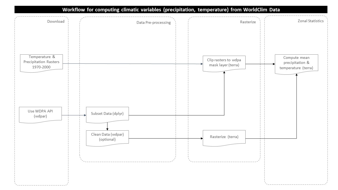
Processing Workflow
The purpose of this analysis is to compute average temperature and average precipitation for the desired polygons. We need to perform zonal statistics operation. A zonal statistics operation is one that calculates statistics on cell values of a raster (a value raster) within the zones defined by another dataset [ArcGIS definition].
To calculate zonal statistics for climatic variables, following processing routine is followed in this analysis:
Download and Prepare WDPA Polygons
For this analysis, we would try to get the country level polygon data from wdpar package. wdpar is a library to interface to the World Database on Protected Areas (WDPA). The library is used to monitor the performance of existing PAs and determine priority areas for the establishment of new PAs. We will use Brazil - for other countries of your choice, simply provide the country name or the ISO name e.g. VEN for Venezuela, Gy for Guyana, COL for Colombia.
# fetch the raw data from wdpar of country
br_wdpa_raw <-
  wdpar::wdpa_fetch("BRA")
Since there are 3202 enlisted protected areas in Brazil (as of time of writing), we want to compute zonal statistics only for the polygon data of: - Reserva Biologica Do Rio Trombetas - wdpaid 43, - Reserva Extrativista Rio Cajari - wdpaid 31776, and - Estacao Ecologica Do Jari - wdpaid 4891
For this, we have to subset the country level polygon data to the pa level.
# subset three wdpa polygons by their wdpa ids
br_wdpa_subset <-
  br_wdpa_raw%>%
  filter(WDPAID %in% c(43,31776,4891))
Now, we will reproject the polygon data to the WGS84 and then apply vect function from terra package to further use it for terra functionalities.
# reproject to the WGS84
br_wdpa_subset <- st_transform(br_wdpa_subset,
                               "+proj=longlat +datum=WGS84 +no_defs")
# spatvector for terra compatibility
br_wdpa_subset_v <-
  vect(br_wdpa_subset)
# we can plot the data to see the three selected polygons
plot(br_wdpa_subset[1])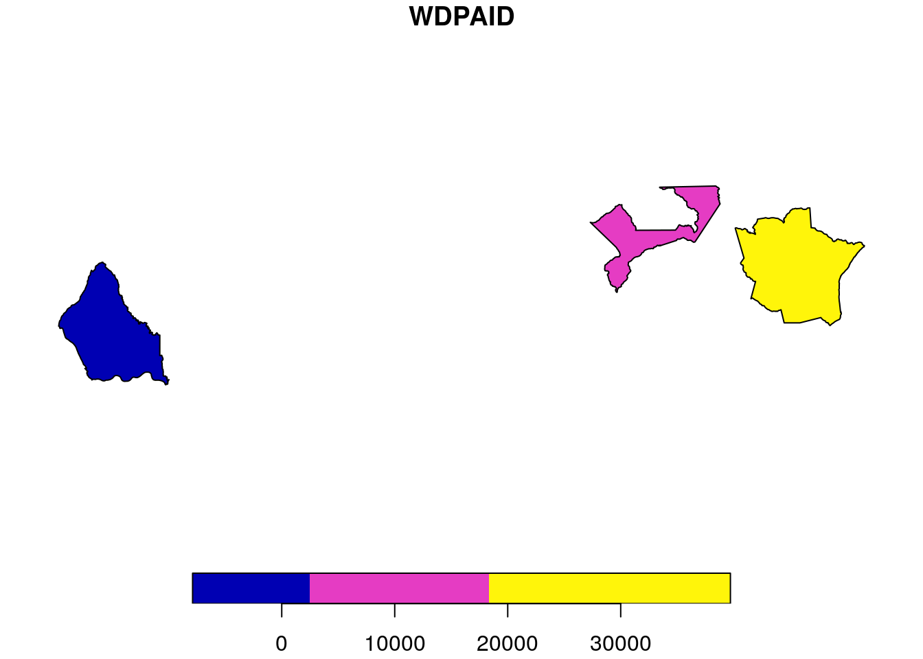
Prepare precipitation and temperature raster data
The global rasters (precipitation, average temperature) aggregated monthly for years 1970-2000 were downloaded in our directory in datalake. Here, we are going to load the tavg and prec raster layers for the month of January using package terra.
# load precipitation raster
prec_rast <-
  terra::rast("../../datalake/mapme.protectedareas/input/precipitation/wc2.1_30s_prec_01.tif")
# view raster details
prec_rast
class : SpatRaster
dimensions : 21600, 43200, 1 (nrow, ncol, nlyr)
resolution : 0.008333333, 0.008333333 (x, y)
extent : -180, 180, -90, 90 (xmin, xmax, ymin, ymax)
coord. ref. : lon/lat WGS 84 (EPSG:4326)
source : wc2.1_30s_prec_01.tif
name : wc2.1_30s_prec_01
min value : 0
max value : 973 # load temperature raster
tavg_rast <-
terra::rast("../../datalake/mapme.protectedareas/input/temperature/wc2.1_30s_tavg_01.tif")
# view raster details
tavg_rastclass : SpatRaster
dimensions : 21600, 43200, 1 (nrow, ncol, nlyr)
resolution : 0.008333333, 0.008333333 (x, y)
extent : -180, 180, -90, 90 (xmin, xmax, ymin, ymax)
coord. ref. : lon/lat WGS 84 (EPSG:4326)
source : wc2.1_30s_tavg_01.tif
name : wc2.1_30s_tavg_01
min value : -46.1
max value : 34.1 Crop the rasters
As we completed raster and polygon data preparation, the next step would be to crop the raster layer by the selected protected areas polygon both by its extent and mask layer. If we apply function crop, it gives us the raster layer by extent. However, using mask function returns the raster to defined vector polygon layer, which is required for zonal statistics computation.
# crop raster by polygon (tavg)
tavg_rast_crop <-
        terra::crop(tavg_rast,
                    br_wdpa_subset_v)
# plot the cropped raster layer (tavg)
plot(tavg_rast_crop)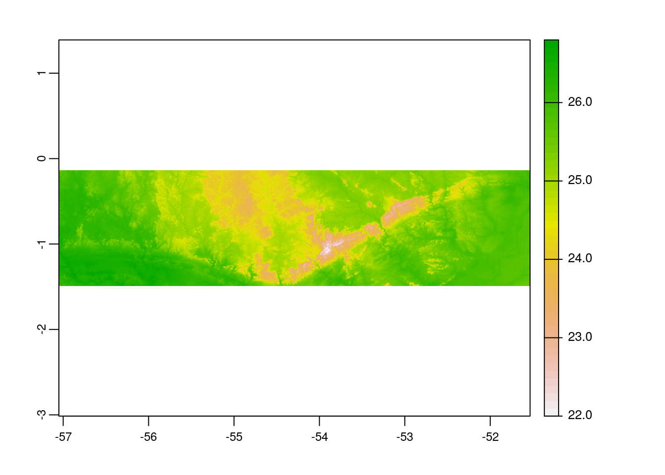
# mask the raster by polygon (tavg)
tavg_rast_mask <-
        terra::mask(tavg_rast_crop,
                    br_wdpa_subset_v)
# plot the masked raster layer (tavg)
plot(tavg_rast_mask)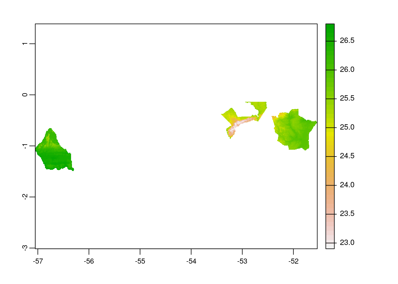
Note: With these above two plots, you can see the difference between the use of functions crop & mask. Thus, always use mask to compute zonal statistics.
Similarly, we will repeat the crop & mask operation for rainfall rasters too.
# crop raster by polygon (prec)
prec_rast_crop <-
        terra::crop(prec_rast,
                    br_wdpa_subset_v)
# mask the raster by polygon (prec)
prec_rast_mask <-
        terra::mask(prec_rast_crop,
                    br_wdpa_subset_v)
Rasterize the polygon layer
To compute the zonal statistics, it is necessary to rasterize the polygon layer. Doing so, values are transferred from the spatial objects to raster cells. We need to pass the extent layer and the mask layer to the rasterize function.
# rasterize the polygon
br_subset_rast <-terra::rasterize(br_wdpa_subset_v,
                                  tavg_rast_mask,
                                  br_wdpa_subset_v$WDPAID)
# plot the rasterized polygon
plot(br_subset_rast)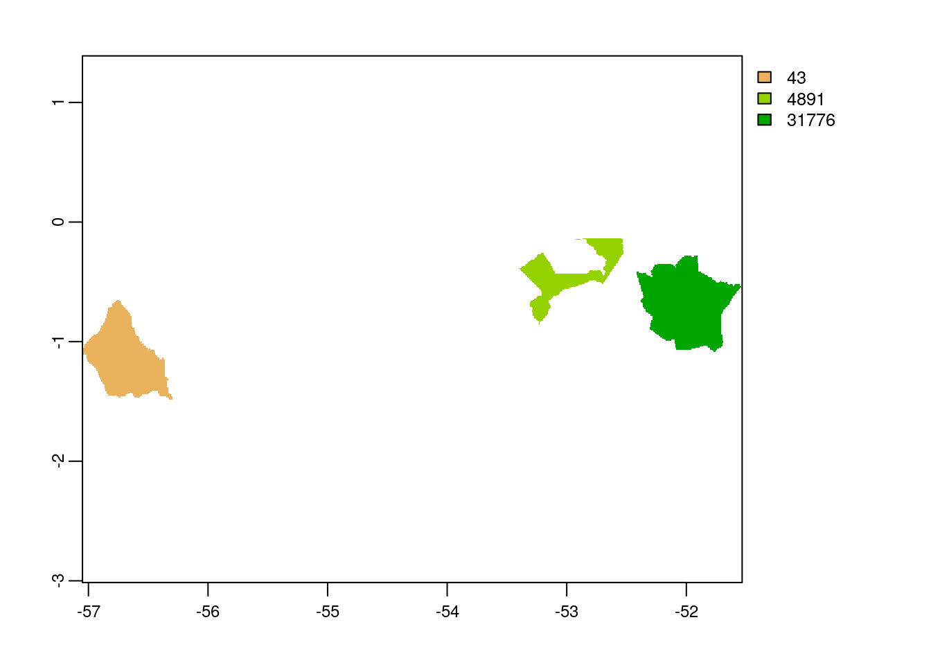
Note: We can use either of the two rasters for rasterize operation since it uses only the resolution and extent from the raster file. So, we don’t need to repeat this step.
Compute Zonal Statistics
A zonal statistics operation is one that calculates statistics on cell values of a raster (a value raster) within the zones defined by another dataset [ArcGIS definition]. Here, we are interested only on computation of the average temperature and average precipitation values, so, we would use function mean for zonal operation.
# zonal stats (mean temperature)
zstats_tavg <- terra::zonal(tavg_rast_mask,
                            br_subset_rast,
                            fun='mean',
                            na.rm=T)
# zonal stats (mean precipitation)
zstats_prec <- terra::zonal(prec_rast_mask,
                            br_subset_rast,
                            fun='mean',
                            na.rm=T)
Now that we computed zonal statistics for both mean precipitation and mean temperature, lets tidy up the dataframe a bit and view the results in more readble form.
# create new dataframe with the values from zonal statistics
df.zstats <- data.frame(WDPAID=br_wdpa_subset$WDPAID,
                        mean_temperature_January=zstats_tavg[ ,2],
                        mean_precipitation_January=zstats_prec[ ,2])
# view the data
df.zstats
WDPAID mean_temperature_January mean_precipitation_January
1 43 26.34158 257.1003
2 4891 24.66911 243.2081
3 31776 25.63760 262.2386From the zonal statistics result, we can see that the polygon with wdpaid 43 has highest temperature among these three whereas polygon with wdpaid 31776 has more rainfall. In this way, we can compute mean temperature and mean precipitation values for our defined region of interest.
In the end we are going to have a look how long the rendering of this file took to get an idea about the processing speed of this routine.
stoptime <-
  Sys.time()
print(stoptime - starttime)
Time difference of 15.28279 secsReferences
[1] Fick, S.E. and R.J. Hijmans, 2017. WorldClim 2: new 1km spatial resolution climate surfaces for global land areas. International Journal of Climatology 37 (12): 4302-4315.
sessionInfo()R version 3.6.3 (2020-02-29)
Platform: x86_64-pc-linux-gnu (64-bit)
Running under: Ubuntu 18.04.6 LTS
Matrix products: default
BLAS: /usr/lib/x86_64-linux-gnu/blas/libblas.so.3.7.1
LAPACK: /usr/lib/x86_64-linux-gnu/lapack/liblapack.so.3.7.1
locale:
[1] LC_CTYPE=C.UTF-8 LC_NUMERIC=C LC_TIME=C.UTF-8
[4] LC_COLLATE=C.UTF-8 LC_MONETARY=C.UTF-8 LC_MESSAGES=C.UTF-8
[7] LC_PAPER=C.UTF-8 LC_NAME=C LC_ADDRESS=C
[10] LC_TELEPHONE=C LC_MEASUREMENT=C.UTF-8 LC_IDENTIFICATION=C
attached base packages:
[1] stats graphics grDevices utils datasets methods base
other attached packages:
[1] forcats_0.5.1 stringr_1.4.0 dplyr_1.0.7 purrr_0.3.4
[5] readr_1.4.0 tidyr_1.1.4 tibble_3.1.6 ggplot2_3.3.4
[9] tidyverse_1.3.1 wdpar_1.3.2 terra_1.5-2 sf_1.0-4
loaded via a namespace (and not attached):
[1] bitops_1.0-6 fs_1.5.0 lubridate_1.7.10 httr_1.4.2
[5] rprojroot_2.0.2 tools_3.6.3 backports_1.2.1 bslib_0.2.5.1
[9] utf8_1.2.2 R6_2.5.1 KernSmooth_2.23-20 DBI_1.1.1
[13] colorspace_2.0-1 withr_2.4.2 tidyselect_1.1.1 processx_3.5.2
[17] curl_4.3.2 compiler_3.6.3 git2r_0.28.0 cli_3.1.0
[21] rvest_1.0.0 xml2_1.3.2 sass_0.4.0 caTools_1.18.1
[25] scales_1.1.1 classInt_0.4-3 proxy_0.4-26 askpass_1.1
[29] rappdirs_0.3.3 digest_0.6.27 rmarkdown_2.11 wdman_0.2.5
[33] pkgconfig_2.0.3 htmltools_0.5.1.1 dbplyr_2.1.1 highr_0.8
[37] rlang_0.4.12 readxl_1.3.1 rstudioapi_0.13 jquerylib_0.1.4
[41] generics_0.1.1 jsonlite_1.7.2 magrittr_2.0.1 Rcpp_1.0.7
[45] munsell_0.5.0 fansi_0.5.0 lifecycle_1.0.1 stringi_1.7.6
[49] yaml_2.2.1 grid_3.6.3 promises_1.2.0.1 crayon_1.4.2
[53] semver_0.2.0 haven_2.3.1 hms_1.1.1 knitr_1.34
[57] ps_1.5.0 pillar_1.6.4 codetools_0.2-18 reprex_2.0.0
[61] XML_3.99-0.3 glue_1.5.1 evaluate_0.14 modelr_0.1.8
[65] vctrs_0.3.8 httpuv_1.6.1 cellranger_1.1.0 gtable_0.3.0
[69] openssl_1.4.5 assertthat_0.2.1 xfun_0.24 binman_0.1.2
[73] broom_0.7.6 countrycode_1.2.0 e1071_1.7-9 later_1.2.0
[77] class_7.3-19 RSelenium_1.7.7 workflowr_1.6.2 units_0.7-2
[81] ellipsis_0.3.2