Population Count
Om Prakash Bhandari (Author), Johannes Schielein (Review)
5/13/2021
Last updated: 2021-09-15
Checks: 7 0
Knit directory: mapme.protectedareas/
This reproducible R Markdown analysis was created with workflowr (version 1.6.2). The Checks tab describes the reproducibility checks that were applied when the results were created. The Past versions tab lists the development history.
Great! Since the R Markdown file has been committed to the Git repository, you know the exact version of the code that produced these results.
Great job! The global environment was empty. Objects defined in the global environment can affect the analysis in your R Markdown file in unknown ways. For reproduciblity it’s best to always run the code in an empty environment.
The command set.seed(20210305) was run prior to running the code in the R Markdown file. Setting a seed ensures that any results that rely on randomness, e.g. subsampling or permutations, are reproducible.
Great job! Recording the operating system, R version, and package versions is critical for reproducibility.
Nice! There were no cached chunks for this analysis, so you can be confident that you successfully produced the results during this run.
Great job! Using relative paths to the files within your workflowr project makes it easier to run your code on other machines.
Great! You are using Git for version control. Tracking code development and connecting the code version to the results is critical for reproducibility.
The results in this page were generated with repository version 2fc3683. See the Past versions tab to see a history of the changes made to the R Markdown and HTML files.
Note that you need to be careful to ensure that all relevant files for the analysis have been committed to Git prior to generating the results (you can use wflow_publish or wflow_git_commit). workflowr only checks the R Markdown file, but you know if there are other scripts or data files that it depends on. Below is the status of the Git repository when the results were generated:
Ignored files:
    Ignored:    .RData
    Ignored:    .Rhistory
    Ignored:    .Rproj.user/
    Ignored:    data-raw/addons/docs/rest/
    Ignored:    data-raw/addons/etc/
    Ignored:    data-raw/addons/scripts/

Untracked files:
    Untracked:  .tmp/
Note that any generated files, e.g. HTML, png, CSS, etc., are not included in this status report because it is ok for generated content to have uncommitted changes.
These are the previous versions of the repository in which changes were made to the R Markdown (analysis/worldpop-population-count.rmd) and HTML (docs/worldpop-population-count.html) files. If you’ve configured a remote Git repository (see ?wflow_git_remote), click on the hyperlinks in the table below to view the files as they were in that past version.
| File | Version | Author | Date | Message |
|---|---|---|---|---|
| html | d1cfe2d | Johannes Schielein | 2021-09-15 | initial comit with sampling code |
| Rmd | b589068 | Ohm-Np | 2021-07-03 | update author names, urls & source code description |
| html | 1468f42 | Ohm-Np | 2021-07-03 | update html files |
| html | fa42f34 | Johannes Schielein | 2021-07-01 | Host with GitHub. |
| html | 8bd1321 | Johannes Schielein | 2021-06-30 | Host with GitLab. |
| html | 3a39ee3 | Johannes Schielein | 2021-06-30 | Host with GitHub. |
| html | ae67dca | Johannes Schielein | 2021-06-30 | Host with GitLab. |
| html | a884b03 | Om Bandhari | 2021-06-30 | update html for index rmd |
| Rmd | 84b8824 | Om Bandhari | 2021-06-30 | update rmd analysis |
| html | 1501982 | Ohm-Np | 2021-05-14 | minor updates index/docs |
| Rmd | ab80285 | Ohm-Np | 2021-05-14 | create worldpop population count rmd |
# load required libraries
library("sf")
library("terra")
library("wdpar")
library("tidyverse")

starttime<-Sys.time() # mark the start time of this routine to calculate processing time at the end
Introduction
Anthropogenic disturbance to the protected areas is a well-known issue to all environmentalists and those working on the conservation of protected areas. To analyze the effect of human population pressure towards the protected areas, it is of utmost importance to get the idea of the number of the human population residing within the protected areas and in the vicinity of those areas. A figure demonstrating the human population and the change on those figures throughout the years assist in making an empirical analysis of the human population pressure to the protected areas. For this, it is necessary to get the most reliable and high-quality datasets. WorldPop, which was initiated in 2013, offers easy access to spatial demographic datasets, claiming to use peer-reviewed and fully transparent methods to create global mosaics for the years 2000 to 2020, which we will use here in this analysis.
Datasource and Metadata Information
- Dataset: - WorldPop Unconstrained Global Mosaics
- Geographical Coverage: Global
- Spatial resolution: 1Km
- Temporal Coverage: 2000-2020
- Temporal resolution: Annual Updates
- Unit: number of people per grid cell
- Data downloaded: 5th May, 2021
- Metadata Link
- Download Link
Processing Workflow
The purpose of this analysis is to compute the number of people residing in a particular protected area’s polygon of interest. In order to obtain the result, we need to go through several steps of processing as shown in the routine workflow:
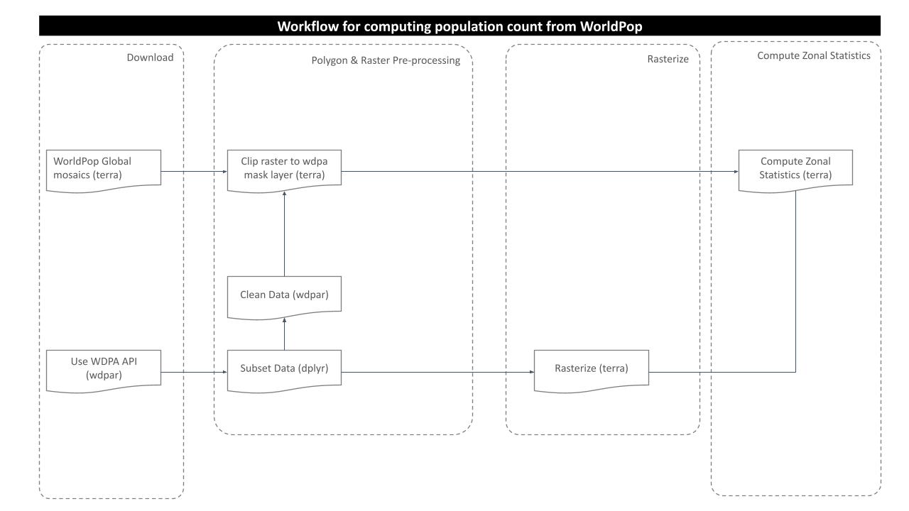
Prepare population count raster
Among all the available global rasters for years 2000 to 2020 were downloaded, for this routine, we would only use for a particular year i.e. 2000.
# load global mosaic - population count raster
pop <-
  rast("../../datalake/mapme.protectedareas/input/world_pop/global_mosaic2000.tif")
# plot raster
plot(pop)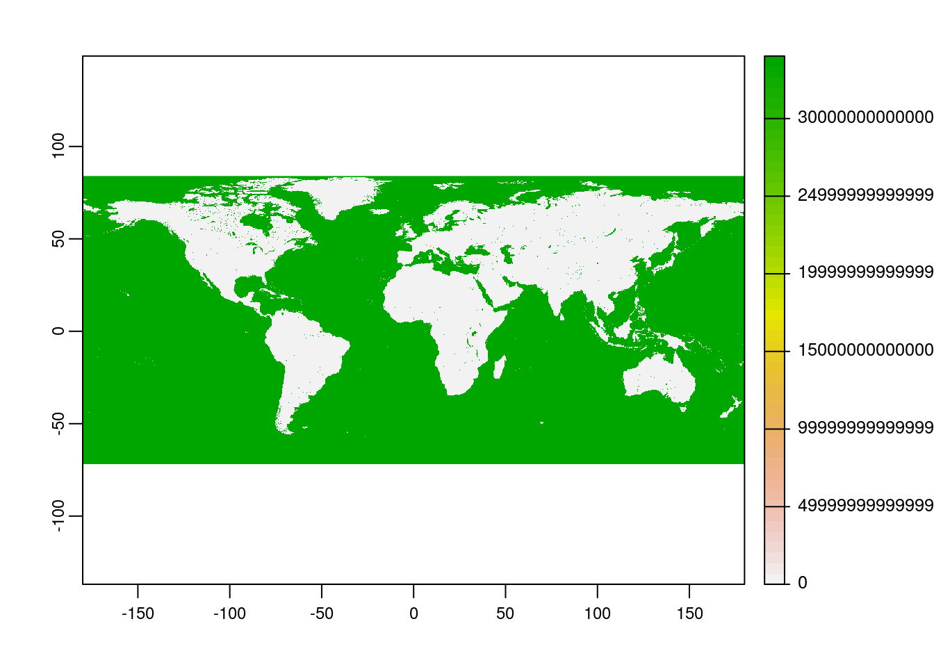
Prepare WDPA Polygon
Since we already prepared raster data for our analysis. Now, we will try to get the country level polygon data from wdpar package. wdpar is a library to interface to the World Database on Protected Areas (WDPA). The library is used to monitor the performance of existing PAs and determine priority areas for the establishment of new PAs. We will use Brazil - for other countries of your choice, simply provide the country name or the ISO name e.g. Gy for Guyana, COL for Colombia.
# fetch the raw data from wdpar of country
br_raw_pa_data <-
  wdpa_fetch("BRA")
Since there are multiple enlisted protected areas in Brazil, we want to compute zonal statistics only for the polygon data of: - Reserva Extrativista Rio Cajari - wdpaid 31776 and - Estacao Ecologica Do Jari - wdpaid 4891
For this, we have to subset the country level polygon data to the PA level.
# subset the wdpa polygons by their wdpa ids
brazil <-
  br_raw_pa_data%>%
  filter(WDPAID %in% c(31776, 4891))
# plot the sample polygon
plot(brazil[1])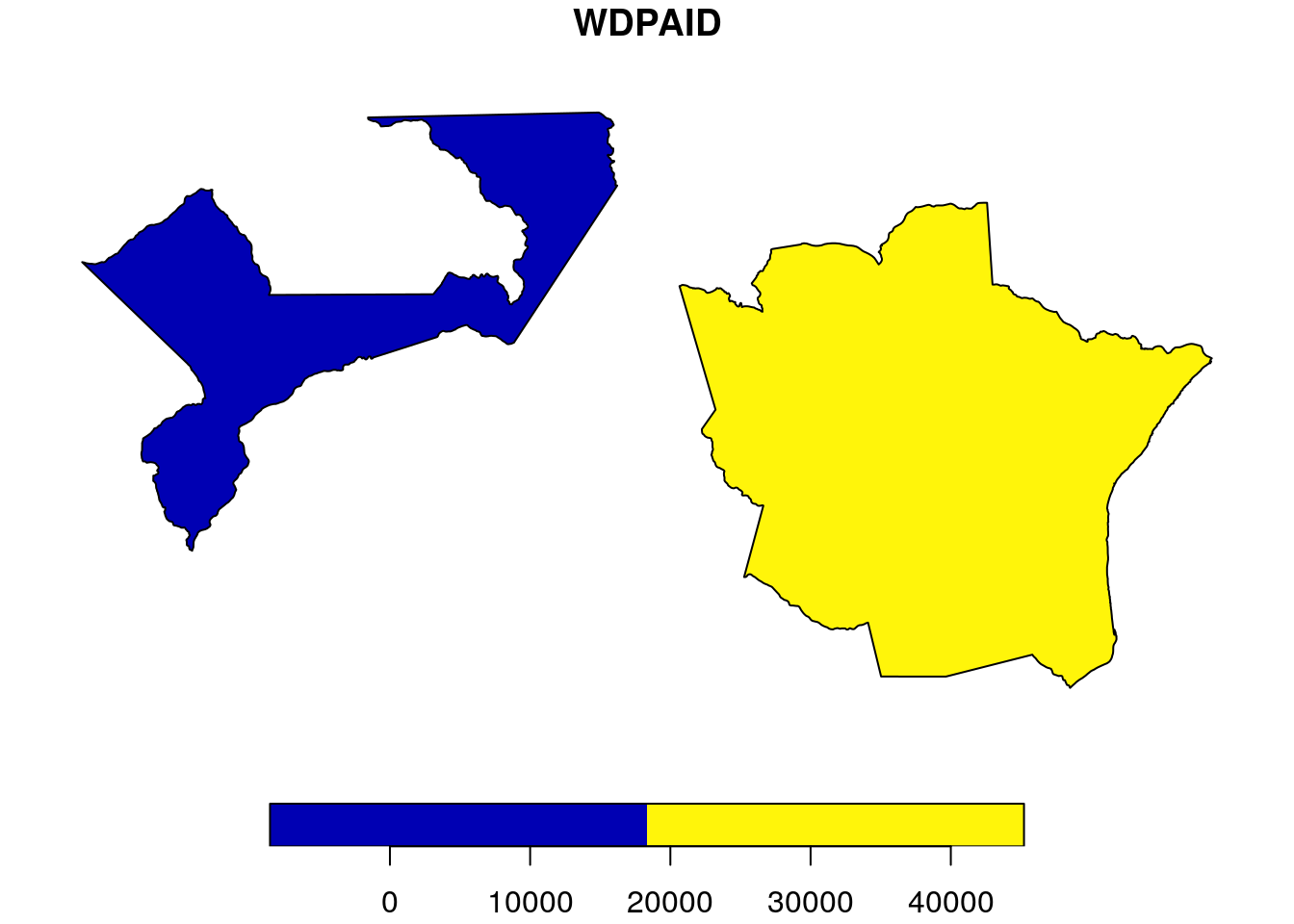
Crop the population count raster
As we completed raster and vector data preparation, the next step would be to clip the raster layer by the selected PA polygon both by its extent and mask layer.
# convert object brazil to spatVector object
bra_v <- as(brazil, "Spatial")%>%
  vect()
# crop raster using polygon extent
myCrop <- terra::crop(pop,
                      bra_v)
# plot the data - shows the raster after getting cropped by the extent of polygon
plot(myCrop)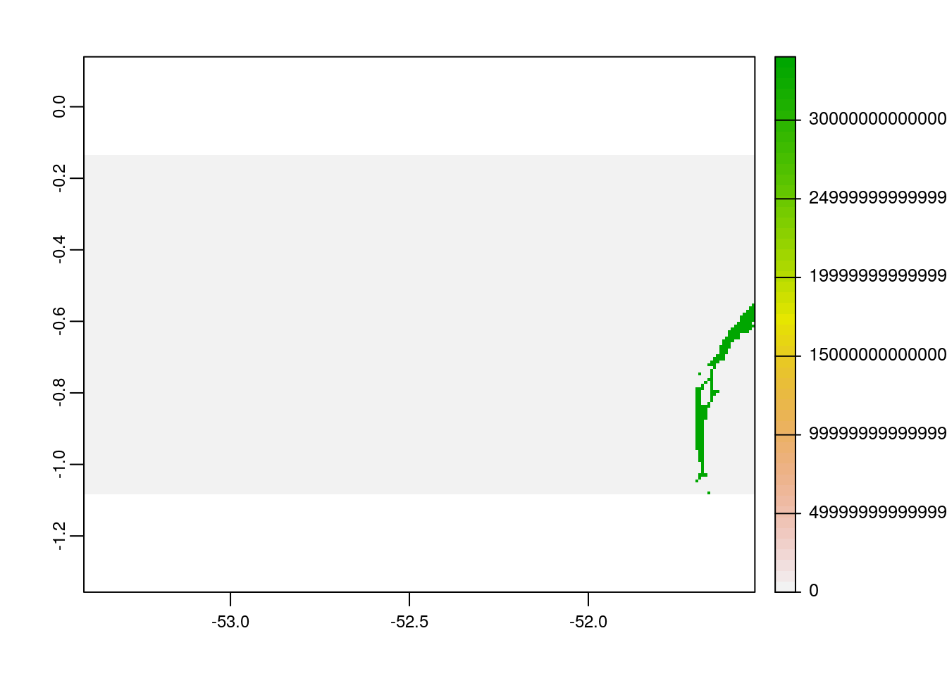
# crop raster using polygon mask
myMask <- mask(myCrop,
               bra_v)
# plot the data - shows the raster after getting cropped by the polygon mask
plot(myMask)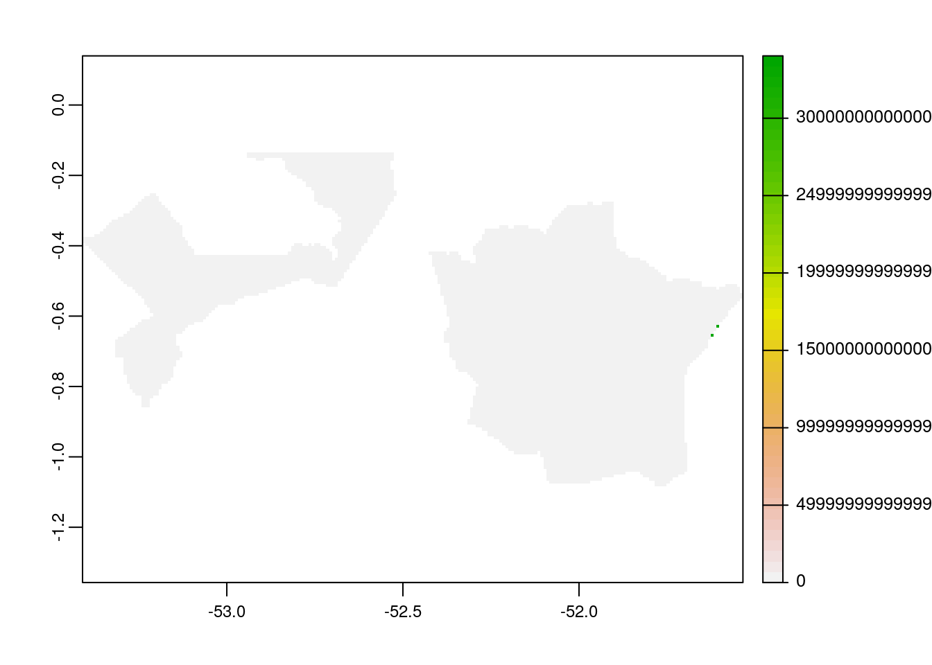
Rasterize the polygon layer
To compute the zonal statistics, it is necessary to rasterize the polygon layer. Doing so, values are transferred from the spatial objects to raster cells. We need to pass the extent layer and the mask layer to the rasterize function.
# rasterize
r <- rasterize(bra_v,
               myMask,
               bra_v$WDPAID)
# view the rasterized polygon
plot(r)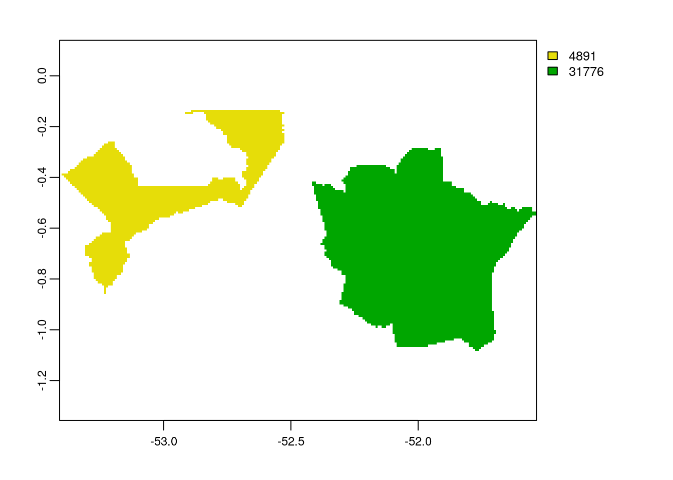
Compute zonal statistics
A zonal statistics operation is one that calculates statistics on cell values of a raster (a value raster) within the zones defined by another dataset [ArcGIS definition].
# zonal stats
zstats <- zonal(myMask, r, fun='sum', na.rm=T)
# view the results
zstats
global_mosaic2000
1 4891 12.0065
2 31776 2908.8636From the result of zonal statistics, we can see the number of people residing in the protected areas with WDPAIDs 4891 and 31776. In a similar way, we can also compute the number of people in a particular region of interest for the desired year and analyze whether the population is following increasing or decreasing trend which helps scientific community to understand the demographic effects towards the protected regions.
In the end we are going to have a look how long the rendering of this file took so that people get an idea about the processing speed of this routine.
stoptime<-Sys.time()
print(starttime-stoptime)
Time difference of -5.409796 secsReferences
[1] Worldpop.org. 2021. WorldPop. [online] Available at: https://www.worldpop.org/ [Accessed 14 May 2021].
sessionInfo()R version 3.6.3 (2020-02-29)
Platform: x86_64-pc-linux-gnu (64-bit)
Running under: Ubuntu 18.04.5 LTS
Matrix products: default
BLAS: /usr/lib/x86_64-linux-gnu/blas/libblas.so.3.7.1
LAPACK: /usr/lib/x86_64-linux-gnu/lapack/liblapack.so.3.7.1
locale:
[1] LC_CTYPE=C.UTF-8 LC_NUMERIC=C LC_TIME=C.UTF-8
[4] LC_COLLATE=C.UTF-8 LC_MONETARY=C.UTF-8 LC_MESSAGES=C.UTF-8
[7] LC_PAPER=C.UTF-8 LC_NAME=C LC_ADDRESS=C
[10] LC_TELEPHONE=C LC_MEASUREMENT=C.UTF-8 LC_IDENTIFICATION=C
attached base packages:
[1] stats graphics grDevices utils datasets methods base
other attached packages:
[1] forcats_0.5.1 stringr_1.4.0 dplyr_1.0.6 purrr_0.3.4
[5] readr_1.4.0 tidyr_1.1.3 tibble_3.1.1 ggplot2_3.3.4
[9] tidyverse_1.3.1 wdpar_1.0.6 terra_1.2-15 sf_0.9-8
loaded via a namespace (and not attached):
[1] httr_1.4.2 jsonlite_1.7.2 modelr_0.1.8 assertthat_0.2.1
[5] countrycode_1.2.0 sp_1.4-5 cellranger_1.1.0 yaml_2.2.1
[9] pillar_1.6.0 backports_1.2.1 lattice_0.20-44 glue_1.4.2
[13] digest_0.6.27 promises_1.2.0.1 rvest_1.0.0 colorspace_2.0-1
[17] htmltools_0.5.1.1 httpuv_1.6.1 pkgconfig_2.0.3 broom_0.7.6
[21] raster_3.4-13 haven_2.3.1 scales_1.1.1 whisker_0.4
[25] later_1.2.0 git2r_0.28.0 proxy_0.4-26 generics_0.1.0
[29] ellipsis_0.3.2 withr_2.4.2 cli_2.5.0 magrittr_2.0.1
[33] crayon_1.4.1 readxl_1.3.1 evaluate_0.14 fs_1.5.0
[37] fansi_0.5.0 xml2_1.3.2 class_7.3-19 tools_3.6.3
[41] hms_1.0.0 lifecycle_1.0.0 munsell_0.5.0 reprex_2.0.0
[45] compiler_3.6.3 e1071_1.7-7 rlang_0.4.11 classInt_0.4-3
[49] units_0.7-1 grid_3.6.3 rstudioapi_0.13 rappdirs_0.3.3
[53] rmarkdown_2.6 gtable_0.3.0 codetools_0.2-18 DBI_1.1.1
[57] curl_4.3.2 R6_2.5.0 lubridate_1.7.10 knitr_1.30
[61] rgdal_1.5-23 utf8_1.2.1 workflowr_1.6.2 rprojroot_2.0.2
[65] KernSmooth_2.23-20 stringi_1.6.2 Rcpp_1.0.7 vctrs_0.3.8
[69] dbplyr_2.1.1 tidyselect_1.1.1 xfun_0.24