Last updated: 2021-05-14

Checks: 6 1

Knit directory: mapme.protectedareas/

This reproducible R Markdown analysis was created with workflowr (version 1.6.2). The Checks tab describes the reproducibility checks that were applied when the results were created. The Past versions tab lists the development history.

R Markdown file: uncommitted changes

The R Markdown is untracked by Git. To know which version of the R Markdown file created these results, you’ll want to first commit it to the Git repo. If you’re still working on the analysis, you can ignore this warning. When you’re finished, you can run wflow_publish to commit the R Markdown file and build the HTML.

Environment: empty

Great job! The global environment was empty. Objects defined in the global environment can affect the analysis in your R Markdown file in unknown ways. For reproduciblity it’s best to always run the code in an empty environment.

Seed: set.seed(20210305)

The command set.seed(20210305) was run prior to running the code in the R Markdown file. Setting a seed ensures that any results that rely on randomness, e.g. subsampling or permutations, are reproducible.

Session information: recorded

Great job! Recording the operating system, R version, and package versions is critical for reproducibility.

Cache: none

Nice! There were no cached chunks for this analysis, so you can be confident that you successfully produced the results during this run.

File paths: relative

Great job! Using relative paths to the files within your workflowr project makes it easier to run your code on other machines.

Repository version: 137440f

Great! You are using Git for version control. Tracking code development and connecting the code version to the results is critical for reproducibility.

The results in this page were generated with repository version 137440f. See the Past versions tab to see a history of the changes made to the R Markdown and HTML files.

Note that you need to be careful to ensure that all relevant files for the analysis have been committed to Git prior to generating the results (you can use wflow_publish or wflow_git_commit). workflowr only checks the R Markdown file, but you know if there are other scripts or data files that it depends on. Below is the status of the Git repository when the results were generated:


Ignored files:
    Ignored:    .Rproj.user/
    Ignored:    mapme.protectedareas.Rproj
    Ignored:    renv/library/
    Ignored:    renv/staging/

Untracked files:
    Untracked:  ..grd
    Untracked:  ..gri
    Untracked:  analysis/copernicus-land-cover.rmd
    Untracked:  code/big_data_processing.R

Unstaged changes:
    Modified:   code/copernicus-land-cover.R

Note that any generated files, e.g. HTML, png, CSS, etc., are not included in this status report because it is ok for generated content to have uncommitted changes.

There are no past versions. Publish this analysis with wflow_publish() to start tracking its development.

# load required libraries
library("terra")
library("sf")
library("wdpar")
library("dplyr")
library("rmarkdown") # only used for rendering tables  for this website

starttime<-Sys.time() # mark the start time of this routine to calculate processing time at the end

At first you might want to load the source functions for this routine.

source("code/copernicus-land-cover.R")

Introduction

The actual surface cover of ground is known as Land Cover. The land cover data shows us how much of the region is covered by forests, rivers, wetlands, barren land, or urban infrastructure thus allowing the observation of land cover dynamics over a period of time. There are many products available for the analysis of global land cover classes, however, the European Union’s Earth Observation programme called as Copernicus provides high quality, readily available land cover products from year 2015 to 2019 free of cost for the public use.

Here, in this analysis we are going to compute the area of land cover classes within the region of interest from the rasters downloaded from Copernicus Land Cover Viewer.

Datasource and Metadata Information

Dataset: Copernicus Global Land Cover - (Buchhorn et al. (2020))
Geographical Coverage: Global
Spatial resolution: 100 meter
Temporal Coverage: 2015-2019
Temporal resolution: Annual Updates
Unit: Map codes as values
Data downloaded: 23rd April, 2021
Metadata Link
Download Link

Processing Workflow

The purpose of this analysis is to compute area of different land cover classes present in the polygon of interest. In order to get the results, we need to go through several steps of processing as shown in the routine workflow:

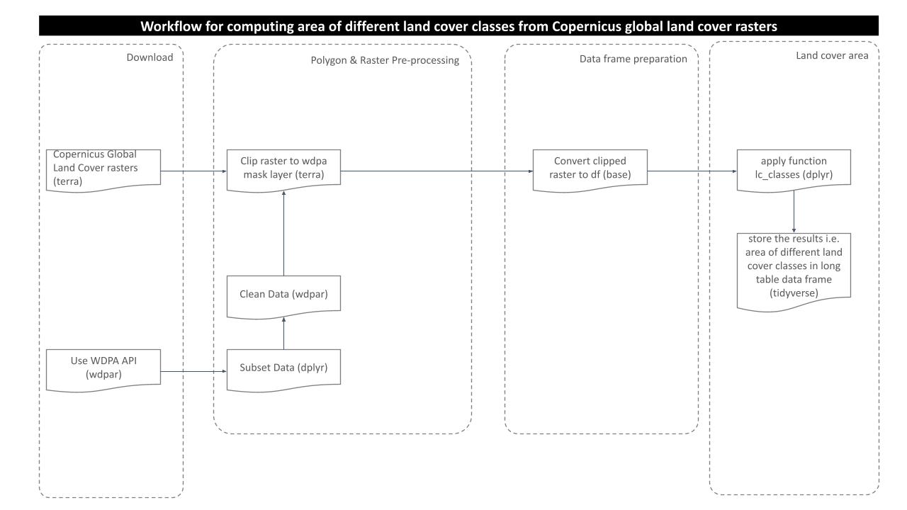
Prepare land cover raster data

The 20X20 gridded rasters were downloaded to cover the extent of Latin America for years 2015 to 2019. Later, for individual years, all the rasters were merged to get the single big raster for particular years. Here, we will load the big raster for the year 2015.

# load raster land cover
lc <- rast("../../datalake/mapme.protectedareas/input/copernicus_global_land_cover/2015/Latin_America_LC_2015.tif")
# view raster details
lc

class       : SpatRaster 
dimensions  : 100800, 100800, 1  (nrow, ncol, nlyr)
resolution  : 0.0009920635, 0.0009920635  (x, y)
extent      : -120, -20, -60, 40  (xmin, xmax, ymin, ymax)
coord. ref. : +proj=longlat +datum=WGS84 +no_defs  
source      : Latin_America_LC_2015.tif 
name        : W040N00 
min value   :       0 
max value   :     200

Download and Prepare WDPA Polygons

For this analysis, we would choose one WDPA polygon from the country Venezuela. We can download the WDPA polygons from the package wdpar and then filter out the desired polygon using WDPAID with package dplyr.

We will then reproject the downloaded polygon sample to WGS84 to match with the raster data. Since, we are using package terra for raster processing, so it is necessary to load the sample polygon as spatVector.

# load sample WDPA polygon from country: Venezuela
ven <- wdpa_fetch("VEN")%>%
  filter(WDPAID %in% 555705224)
# reproject to the WGS84
ven <- st_transform(ven, "+proj=longlat +datum=WGS84 +no_defs")
# load as spatVector for terra compatiility
ven_v <- vect(ven)
# plot the PA polygon
plot(ven[1])

Crop the land cover raster

Since we already loaded raster and polygon successfully to our workspace, we can now perform further processing that would be to clip the raster layer by the selected shapefile polygon both by its extent and mask layer. Crop returns the raster to its bounding box whereas mask returns the raster to defined vector polygon layer.

# crop raster by polygon
ven_crop <- terra::crop(lc, ven_v)
# plot the cropped raster layer
plot(ven_crop)

# mask the raster by polygon 
ven_mask <- terra::mask(ven_crop, ven_v)
# plot the masked raster layer
plot(ven_mask)

Prepare data frame

The next step would be to prepare the data frame. First, we would load the raster values from masked raster layer to the data frame named df.ven. Then, replace the column name containing raster values to value with the use of new data frame called df.new.

# raster values as dataframe
df.ven <- as.data.frame(ven_mask)
# new dataframe with value column
df.new <- data.frame(value=NA)
# rename column to match with new df
colnames(df.ven) <- colnames(df.new)
# check the columns with values of the prepared dataframe
head(df.ven)

Similarly, we will prepare new data frame with only WDPAID to receive the final results.

# empty data frame to receive results
df.final <- data.frame(WDPAID=555705224)

Compute area of land cover classes

To carry out the final and main step of this analysis i.e. to compute the area of land cover classes, area function from the package terra would be used. We first compute the area of the masked raster layer ven_mask in square kilometer (sqkm). Then, we calculate the area in sqkm for single row of the data frame df.ven.

# area of masked raster
area_sqm <- terra::area(ven_mask)
# in sqkm
area_sqkm <- area_sqm/1000000
# area per row of dataframe
area_sqkm_per_cell <- area_sqkm/nrow(df.ven)

Finally, we call the function lc_clases from the sourced script copernicus-land-cover.R which takes the data frame df.ven as argument and returns another data frame data.final in long table format with the area of individual land cover classes.

# call the function lc_classes and receive the result
df.final_long <- lc_classes(df.ven)
# view the resulting data
df.final_long

# A tibble: 23 x 3
      WDPAID name                                                          value
       <dbl> <chr>                                                         <dbl>
 1 555705224 copernicus_lc_empty_area_sqkm_2015                          9.67e-1
 2 555705224 copernicus_lc_closed_forest_evergreen_needle_leaf_area_sqk… 0      
 3 555705224 copernicus_lc_closed_forest_deciduous_needle_leaf_area_sqk… 0      
 4 555705224 copernicus_lc_closed_forest_evergreen_broad_leaf_area_sqkm… 9.82e+3
 5 555705224 copernicus_lc_closed_forest_deciduous_broad_leaf_area_sqkm… 1.14e+2
 6 555705224 copernicus_lc_closed_forest_mixed_area_sqkm_2015            0      
 7 555705224 copernicus_lc_closed_forest_unknown_area_sqkm_2015          1.93e+3
 8 555705224 copernicus_lc_open_forest_evergreen_needle_leaf_area_sqkm_… 0      
 9 555705224 copernicus_lc_open_forest_deciduous_needle_leaf_area_sqkm_… 0      
10 555705224 copernicus_lc_open_forest_evergreen_broad_leaf_area_sqkm_2… 1.18e+3
# … with 13 more rows

So, for a single polygon for the year 2015, we computed the area of each land cover classes present in the polygon. We can see that among 23 discrete classes, the polygon we used consists of eight different classes with open forest comprising the largest area of the polygon.

In order to carry out land cover change analysis, we can load raster layer for another year of which we want to see the changes in the area of land cover classes and then finally subtract the area from the respective years.

In the end we are going to have a look how long the rendering of this file took so that people get an idea about the processing speed of this routine.

stoptime<-Sys.time()
print(starttime-stoptime)

Time difference of -12.8952 secs

References

[1] Buchhorn, M. ; Smets, B. ; Bertels, L. ; De Roo, B. ; Lesiv, M. ; Tsendbazar, N. - E. ; Herold, M. ; Fritz, S. Copernicus Global Land Service: Land Cover 100m: collection 3: epoch 2019: Globe 2020. DOI 10.5281/zenodo.3939050

[2] Buchhorn, M. ; Smets, B. ; Bertels, L. ; De Roo, B. ; Lesiv, M. ; Tsendbazar, N. - E. ; Herold, M. ; Fritz, S. Copernicus Global Land Service: Land Cover 100m: collection 3: epoch 2018: Globe 2020. DOI 10.5281/zenodo.3518038

[3] Buchhorn, M. ; Smets, B. ; Bertels, L. ; De Roo, B. ; Lesiv, M. ; Tsendbazar, N. - E. ; Herold, M. ; Fritz, S. Copernicus Global Land Service: Land Cover 100m: collection 3: epoch 2017: Globe 2020. DOI 10.5281/zenodo.3518036

[4]Buchhorn, M. ; Smets, B. ; Bertels, L. ; De Roo, B. ; Lesiv, M. ; Tsendbazar, N. - E. ; Herold, M. ; Fritz, S. Copernicus Global Land Service: Land Cover 100m: collection 3: epoch 2016: Globe 2020. DOI 10.5281/zenodo.3518026

[5] Buchhorn, M. ; Smets, B. ; Bertels, L. ; De Roo, B. ; Lesiv, M. ; Tsendbazar, N. - E. ; Herold, M. ; Fritz, S. Copernicus Global Land Service: Land Cover 100m: collection 3: epoch 2015: Globe 2020. DOI 10.5281/zenodo.3939038

sessionInfo()

R version 4.0.0 (2020-04-24)
Platform: x86_64-pc-linux-gnu (64-bit)
Running under: Ubuntu 18.04.5 LTS

Matrix products: default
BLAS/LAPACK: /usr/lib/x86_64-linux-gnu/libopenblasp-r0.2.20.so

locale:
 [1] LC_CTYPE=en_US.UTF-8       LC_NUMERIC=C              
 [3] LC_TIME=en_US.UTF-8        LC_COLLATE=en_US.UTF-8    
 [5] LC_MONETARY=en_US.UTF-8    LC_MESSAGES=C             
 [7] LC_PAPER=en_US.UTF-8       LC_NAME=C                 
 [9] LC_ADDRESS=C               LC_TELEPHONE=C            
[11] LC_MEASUREMENT=en_US.UTF-8 LC_IDENTIFICATION=C       

attached base packages:
[1] stats     graphics  grDevices datasets  utils     methods   base     

other attached packages:
 [1] forcats_0.5.1   stringr_1.4.0   purrr_0.3.4     readr_1.4.0    
 [5] tidyr_1.1.3     tibble_3.1.1    ggplot2_3.3.3   tidyverse_1.3.1
 [9] rmarkdown_2.7   dplyr_1.0.5     wdpar_1.0.6     sf_0.9-8       
[13] terra_1.2-5     workflowr_1.6.2

loaded via a namespace (and not attached):
 [1] httr_1.4.2         jsonlite_1.7.2     modelr_0.1.8       assertthat_0.2.1  
 [5] countrycode_1.2.0  sp_1.4-5           highr_0.9          renv_0.13.0       
 [9] cellranger_1.1.0   yaml_2.2.1         pillar_1.6.0       backports_1.2.1   
[13] lattice_0.20-41    glue_1.4.2         digest_0.6.27      promises_1.2.0.1  
[17] rvest_1.0.0        colorspace_2.0-1   htmltools_0.5.1.1  httpuv_1.6.0      
[21] pkgconfig_2.0.3    broom_0.7.6        raster_3.4-10      haven_2.4.1       
[25] scales_1.1.1       later_1.2.0        git2r_0.28.0       proxy_0.4-25      
[29] generics_0.1.0     ellipsis_0.3.2     withr_2.4.2        cli_2.5.0         
[33] magrittr_2.0.1     crayon_1.4.1       readxl_1.3.1       evaluate_0.14     
[37] fs_1.5.0           fansi_0.4.2        xml2_1.3.2         class_7.3-16      
[41] tools_4.0.0        hms_1.0.0          lifecycle_1.0.0    munsell_0.5.0     
[45] reprex_2.0.0       compiler_4.0.0     e1071_1.7-6        rlang_0.4.11      
[49] classInt_0.4-3     units_0.7-1        grid_4.0.0         rstudioapi_0.13   
[53] rappdirs_0.3.3     gtable_0.3.0       codetools_0.2-16   DBI_1.1.1         
[57] curl_4.3.1         R6_2.5.0           lubridate_1.7.10   knitr_1.33        
[61] utf8_1.2.1         rprojroot_2.0.2    KernSmooth_2.23-16 stringi_1.5.3     
[65] Rcpp_1.0.6         vctrs_0.3.8        dbplyr_2.1.1       tidyselect_1.1.1  
[69] xfun_0.22

Copernicus Global Land Cover

Johannes Schielein, Om Prakash Bhandari

5/4/2021