Processing Terrestrial Ecoregions of the World(TEOW)
Johannes Schielein, Om Prakash Bhandari
3/12/2021
Last updated: 2021-03-15
Checks: 5 2
Knit directory: mapme.protectedareas/
This reproducible R Markdown analysis was created with workflowr (version 1.6.2). The Checks tab describes the reproducibility checks that were applied when the results were created. The Past versions tab lists the development history.
The R Markdown is untracked by Git. To know which version of the R Markdown file created these results, you’ll want to first commit it to the Git repo. If you’re still working on the analysis, you can ignore this warning. When you’re finished, you can run wflow_publish to commit the R Markdown file and build the HTML.
Great job! The global environment was empty. Objects defined in the global environment can affect the analysis in your R Markdown file in unknown ways. For reproduciblity it’s best to always run the code in an empty environment.
The command set.seed(20210305) was run prior to running the code in the R Markdown file. Setting a seed ensures that any results that rely on randomness, e.g. subsampling or permutations, are reproducible.
Great job! Recording the operating system, R version, and package versions is critical for reproducibility.
Nice! There were no cached chunks for this analysis, so you can be confident that you successfully produced the results during this run.
Using absolute paths to the files within your workflowr project makes it difficult for you and others to run your code on a different machine. Change the absolute path(s) below to the suggested relative path(s) to make your code more reproducible.
| absolute | relative |
|---|---|
| /home/ombhandari/shared/Om/mapme.protectedareas/ | . |
Great! You are using Git for version control. Tracking code development and connecting the code version to the results is critical for reproducibility.
The results in this page were generated with repository version 1712d4d. See the Past versions tab to see a history of the changes made to the R Markdown and HTML files.
Note that you need to be careful to ensure that all relevant files for the analysis have been committed to Git prior to generating the results (you can use wflow_publish or wflow_git_commit). workflowr only checks the R Markdown file, but you know if there are other scripts or data files that it depends on. Below is the status of the Git repository when the results were generated:
Ignored files:
    Ignored:    .Rproj.user/
    Ignored:    mapme.protectedareas.Rproj
    Ignored:    mytempdir/
    Ignored:    renv/library/
    Ignored:    renv/staging/

Untracked files:
    Untracked:  analysis/figure/
    Untracked:  analysis/wwf_teow.rmd
    Untracked:  code/area_proj.R
    Untracked:  data/Terrestrial_Ecoregions_World.cpg
    Untracked:  data/Terrestrial_Ecoregions_World.dbf
    Untracked:  data/Terrestrial_Ecoregions_World.prj
    Untracked:  data/Terrestrial_Ecoregions_World.shp
    Untracked:  data/Terrestrial_Ecoregions_World.shx
Note that any generated files, e.g. HTML, png, CSS, etc., are not included in this status report because it is ok for generated content to have uncommitted changes.
There are no past versions. Publish this analysis with wflow_publish() to start tracking its development.
knitr::opts_knit$set(root.dir = "/home/ombhandari/shared/Om/mapme.protectedareas/")
# load required libraries
library("sp")
library("sf")
library("wdpar")
library("dplyr")
library("rmapshaper")
library("rmarkdown")
Introduction
Terrestrial Ecoregions of the World (TEOW) is a biogeographic regionalization of the Earth’s terrestrial biodiversity. Our biogeographic units are ecoregions, which are defined as relatively large units of land or inland water containing a distinct assemblage of natural communities sharing a large majority of species, dynamics, and environmental conditions. There are 867 terrestrial ecoregions, classified into 14 different biomes such as forests, grasslands, or deserts. Ecoregions represent the original distribution of distinct assemblages of species and communities.Visit Link for more information on TEOW from WWF.
Here we are going to carry out an analysis to see the level of intersection of different WDPA polygon layers with the Ecoregions; to answer how much area of wdpa polygon is within a particular type of ecoregion.
To carry out this analysis, we will follow this processing routine:
- fetch country level WDPA polygon from
wdpar - select desired wdpa polygon from
wdparand clean the data - load archived global TEOW polygon
- simplify the TEOW polygon
- generate projstring using
area_projfunction & transfrom the projection system of polygons - intersect TEOW and polygon layer
- extract areas of the intersection
- for each wdpaid, get name of the PA, ecoregion IDs, ecoregion names and area of intersected polygons
WDPA polygon data preparation
First of all, we will try to get the country level polygon data from wdpar package. wdpar is a library to interface to the World Database on Protected Areas (WDPA). The library is used to monitor the performance of existing PAs and determine priority areas for the establishment of new PAs. We will use Brazil - for other countries of your choice, simply provide the country name or the ISO3 name e.g. Gy for Guyana, COL for Colombia
# fetch the raw data from wdpar of country
br_raw_pa_data <- wdpa_fetch("Brazil")
Since there are more than 3000 enlisted protected areas in Brazil, we are interested in only three wdpa polygons: - Reserva Biologica Do Rio Trombetas - wdpaid 43, - Reserva Extrativista Rio Cajari - wdpaid 31776, and - Estacao Ecologica Do Jari - wdpaid 4891
For this, we have to subset the country level polygon data to the pa level.
# subset three wdpa polygons by their wdpa ids
bra<-
  br_raw_pa_data%>%
  filter(WDPAID %in% c(43,4891,31776))
The next immediate step would be to clean the fetched raw data. Cleaning is done so as to:
- exclude protected areas that are not yet implemented
- exclude protected areas with limited conservation value
- replace missing data codes (e.g. “0”) with missing data values (i.e. NA)
- replace protected areas represented as points with circular protected areas that correspond to their reported extent
- repair any topological issues with the geometries
- erase overlapping areas
# clean the data
brac <- wdpa_clean(bra)
# spatial
brac_sp <- as(brac, "Spatial")
In order to generate area statistics, it is important to reproject the polygons from geographic coordinate system to the projected coordinate system. Since we want to preserve the area for this analysis, we will be using Lambert Azimuthal Equal Area Projection. To check the projstring for the desired area of the selection, we call the function area_proj which generates projstring for the supplied feature extent.
At first you should link to the source functions to go through this particular step.
source("code/area_proj.R")Now, call the function to get the required projstring parameters. The function area_proj however only accept sf object.
# # SpatialPolygonsDataFrame for sf compatibility
brac_sf <- st_as_sf(brac_sp)
# apply function
area_proj(brac_sf)
[1] "+proj=laea +lat_0=-103494 +lon_0=-5238465 +x_0=59069094000 +y_0=19274928000 +a=6371007.181 +b=6371007.181 +units=m +no_defs"Now, we will use the above obtained projstring parameters to project our polygon.
# set desired projection to myCrs
myCrs <- "+proj=laea +lat_0=-103494 +lon_0=-5238465 +x_0=59069094000 +y_0=19274928000 +a=6371007.181 +b=6371007.181 +units=m +no_defs"
# transforn the wdpa polygon to the desired projection system
#bra_sft <- st_transform(brac_sf, st_crs(myCrs))
TEOW polygon data preparation
Since, we prepared WDPA polygon data for our analysis, we now load the TEOW global shapefile layer from archived file or if you want to download the teow global shapefile, you can download the file calling the function get_wwf_teow.
# load TEOW global polygons
teow <- read_sf("data/Terrestrial_Ecoregions_World.shp")
# simplify geometry
teow_simp <- ms_simplify(teow)
# SpatialPolygonsDataFrame for sp compatibility
teow_sp <- as(teow_simp, "Spatial")
Intersect TEOW and WDPA Polygon layer
To analyse how much of wdpa area is within which part of the ecoregion, intersection function is applied. st_intersection allows us to see that result. To be able to apply st_intersection, the polygon layers should be saved as sf object. To carry out intersection function, coordinate reference system of both the polygons should be same. For this, we use st_transform to achieve this.
# SpatialPolygonsDataFrame for sf compatibility
teow_sf <- st_as_sf(teow_sp)
# project wdpa polygon to teow
brac_ex <- st_transform(brac_sf, st_crs(teow_sf))
# intersection
teow_pol <- st_intersection(teow_sf, brac_ex)
although coordinates are longitude/latitude, st_intersection assumes that they are planar# plot intersection layer
plot(teow_pol)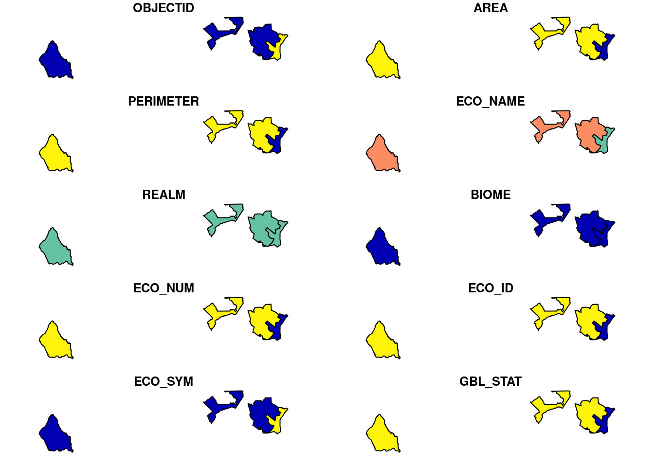
Extract areas and required columns from the intersection layer
Since, we already achieved the intersection, now we want to extract the actual area of interaction between wdpa polygons and teow polygons.
# ectract areas (Sqkm) and save it as new column
teow_pol$Area_Sqm <- st_area(teow_pol)
# tibble - turns existing object to tibble dataframe from library `dplyr`
myData <- as_tibble(teow_pol)
# select only necessary columns from the intersected polygon
myData_f <- myData %>%
  select(WDPAID, NAME, ECO_ID, ECO_NAME, Area_Sqm)
# view the data
myData_f
# A tibble: 4 x 5
WDPAID NAME ECO_ID ECO_NAME Area_Sqm
<dbl> <chr> <int> <chr> [m^2]
1 43 Reserva Biológica Do Rio Tr… 60173 Uatuma-Trombetas moist f… 40773333…
2 4891 Estação Ecológica Do Jari 60173 Uatuma-Trombetas moist f… 23118626…
3 31776 Reserva Extrativista Rio Ca… 60173 Uatuma-Trombetas moist f… 40219160…
4 31776 Reserva Extrativista Rio Ca… 60138 Marajó varzeá 13008450…# with results looking like this in paged table format
paged_table(myData_f)
sessionInfo()R version 4.0.3 (2020-10-10)
Platform: x86_64-pc-linux-gnu (64-bit)
Running under: Ubuntu 20.04 LTS
Matrix products: default
BLAS/LAPACK: /usr/lib/x86_64-linux-gnu/openblas-pthread/libopenblasp-r0.3.8.so
locale:
[1] LC_CTYPE=en_US.UTF-8 LC_NUMERIC=C
[3] LC_TIME=en_US.UTF-8 LC_COLLATE=en_US.UTF-8
[5] LC_MONETARY=en_US.UTF-8 LC_MESSAGES=C
[7] LC_PAPER=en_US.UTF-8 LC_NAME=C
[9] LC_ADDRESS=C LC_TELEPHONE=C
[11] LC_MEASUREMENT=en_US.UTF-8 LC_IDENTIFICATION=C
attached base packages:
[1] stats graphics grDevices utils datasets methods base
other attached packages:
[1] rmarkdown_2.7 rmapshaper_0.4.4 dplyr_1.0.2 wdpar_1.0.6
[5] sf_0.9-7 sp_1.4-5
loaded via a namespace (and not attached):
[1] Rcpp_1.0.6 countrycode_1.2.0 lattice_0.20-41 class_7.3-17
[5] assertthat_0.2.1 rprojroot_2.0.2 digest_0.6.27 utf8_1.1.4
[9] V8_3.4.0 R6_2.5.0 evaluate_0.14 e1071_1.7-4
[13] httr_1.4.2 geojson_0.3.4 highr_0.8 pillar_1.5.0
[17] rlang_0.4.10 lazyeval_0.2.2 curl_4.3 geojsonlint_0.4.0
[21] rstudioapi_0.13 jquerylib_0.1.3 geojsonio_0.9.4 rgdal_1.5-23
[25] foreign_0.8-80 jqr_1.2.0 stringr_1.4.0 compiler_4.0.3
[29] httpuv_1.5.5 xfun_0.21 pkgconfig_2.0.3 rgeos_0.5-5
[33] htmltools_0.5.1.1 tidyselect_1.1.0 tibble_3.1.0 httpcode_0.3.0
[37] workflowr_1.6.2 jsonvalidate_1.1.0 fansi_0.4.2 crayon_1.4.1
[41] later_1.1.0.1 rappdirs_0.3.3 crul_1.1.0 grid_4.0.3
[45] jsonlite_1.7.2 lwgeom_0.2-5 lifecycle_1.0.0 DBI_1.1.1
[49] git2r_0.28.0 magrittr_2.0.1 units_0.7-0 KernSmooth_2.23-17
[53] cli_2.3.1 stringi_1.5.3 fs_1.5.0 promises_1.2.0.1
[57] bslib_0.2.4 ellipsis_0.3.1 generics_0.1.0 vctrs_0.3.6
[61] geojsonsf_2.0.1 tools_4.0.3 glue_1.4.2 purrr_0.3.4
[65] yaml_2.2.1 maptools_1.0-2 classInt_0.4-3 knitr_1.31
[69] sass_0.3.1