Sliced NYC Airbnb

workflowr

• Summary
• Checks
• Past versions

Last updated: 2021-10-11

Checks: 7 0

Knit directory: myTidyTuesday/

This reproducible R Markdown analysis was created with workflowr (version 1.6.2). The Checks tab describes the reproducibility checks that were applied when the results were created. The Past versions tab lists the development history.

---

R Markdown file: up-to-date

Great! Since the R Markdown file has been committed to the Git repository, you know the exact version of the code that produced these results.

Environment: empty

Great job! The global environment was empty. Objects defined in the global environment can affect the analysis in your R Markdown file in unknown ways. For reproduciblity it’s best to always run the code in an empty environment.

Seed: set.seed(20210907)

The command set.seed(20210907) was run prior to running the code in the R Markdown file. Setting a seed ensures that any results that rely on randomness, e.g. subsampling or permutations, are reproducible.

Session information: recorded

Great job! Recording the operating system, R version, and package versions is critical for reproducibility.

Cache: none

Nice! There were no cached chunks for this analysis, so you can be confident that you successfully produced the results during this run.

File paths: relative

Great job! Using relative paths to the files within your workflowr project makes it easier to run your code on other machines.

Repository version: a034f06

Great! You are using Git for version control. Tracking code development and connecting the code version to the results is critical for reproducibility.

The results in this page were generated with repository version a034f06. See the Past versions tab to see a history of the changes made to the R Markdown and HTML files.

Note that you need to be careful to ensure that all relevant files for the analysis have been committed to Git prior to generating the results (you can use wflow_publish or wflow_git_commit). workflowr only checks the R Markdown file, but you know if there are other scripts or data files that it depends on. Below is the status of the Git repository when the results were generated:

Ignored files:
    Ignored:    .Rhistory
    Ignored:    .Rproj.user/
    Ignored:    catboost_info/
    Ignored:    data/2021-09-08/
    Ignored:    data/2021-10-10/
    Ignored:    data/2021-10-11/
    Ignored:    data/CNHI_Excel_Chart.xlsx
    Ignored:    data/CommunityTreemap.jpeg
    Ignored:    data/Community_Roles.jpeg
    Ignored:    data/YammerDigitalDataScienceMembership.xlsx
    Ignored:    data/acs_poverty.rds
    Ignored:    data/airbnbcatboost.rds
    Ignored:    data/australiaweather.rds
    Ignored:    data/fmhpi.rds
    Ignored:    data/grainstocks.rds
    Ignored:    data/hike_data.rds
    Ignored:    data/nber_rs.rmd
    Ignored:    data/netflixTitles.rmd
    Ignored:    data/netflixTitles2.rds
    Ignored:    data/us_states.rds
    Ignored:    data/us_states_hexgrid.geojson
    Ignored:    data/weatherstats_toronto_daily.csv

Untracked files:
    Untracked:  analysis/CHN_1_sp.rds
    Untracked:  analysis/sample data for r test.xlsx
    Untracked:  code/YammerReach.R
    Untracked:  code/work list batch targets.R

Note that any generated files, e.g. HTML, png, CSS, etc., are not included in this status report because it is ok for generated content to have uncommitted changes.

---

These are the previous versions of the repository in which changes were made to the R Markdown (analysis/2021_06_29_sliced.Rmd) and HTML (docs/2021_06_29_sliced.html) files. If you’ve configured a remote Git repository (see ?wflow_git_remote), click on the hyperlinks in the table below to view the files as they were in that past version.

File	Version	Author	Date	Message
Rmd	a034f06	opus1993	2021-10-11	adopt common ggplot theming

---

SLICED is like the TV Show Chopped but for data science. Competitors get a never-before-seen dataset and two-hours to code a solution to a prediction challenge. Contestants get points for the best model plus bonus points for data visualization, votes from the audience, and more.

Season 1 Episode 5 featured a challenge to predict AirBnb pricing for properties in New York City. The evaluation metric in this competition is residual mean log squared error.

To make the best use of the resources that we have, we will explore the data set features to select those with the most predictive power, build a random forest to confirm the recipe, and then use the rest of the time to build one or more catboost ensemble models. Let’s load up some packages:

suppressPackageStartupMessages({
library(tidyverse)
library(hrbrthemes)
library(lubridate)
library(tidytext)

library(tidymodels)
library(textrecipes)
library(treesnip)
library(finetune)
library(stacks)
library(themis)
library(baguette)
  
library(catboost)

})

source(here::here("code","_common.R"),
       verbose = FALSE,
       local = knitr::knit_global())

ggplot2::theme_set(theme_jim(base_size = 12))

#create a data directory
data_dir <- here::here("data",Sys.Date())
if (!file.exists(data_dir)) dir.create(data_dir)

# set a competition metric
mset <- metric_set(mn_log_loss)

# set the competition name from the web address
competition_name <- "sliced-s01e05-WXx7h8"

zipfile <- paste0(data_dir,"/", competition_name, ".zip")

path_export <- here::here("data",Sys.Date(),paste0(competition_name,".csv"))

A quick reminder before downloading the dataset: Go to the web site and accept the competition terms!!!

Import and EDA

I was out on holiday this past week and missed the live competition. This file is a compilation of some of the best parts of what the contestants demonstrated (live coding from scratch) and Julia Silge’s custom metric blog post.

Direct Import and Skim

We have basic shell commands available to interact with Kaggle here:

# from the Kaggle api https://github.com/Kaggle/kaggle-api

# the leaderboard
shell(glue::glue("kaggle competitions leaderboard { competition_name } -s"))

# the files to download
shell(glue::glue("kaggle competitions files -c { competition_name }"))

# the command to download files
shell(glue::glue("kaggle competitions download -c { competition_name } -p { data_dir }"))

# unzip the files received
shell(glue::glue("unzip { zipfile } -d { data_dir }"))

Reading in the contents of the datafiles here:

train_df <-
  read_csv(file = glue::glue(
    {
      data_dir
    },
    "/train.csv"
  )) %>%
  mutate(across(c(id, host_id), as.character)) %>%
  mutate(across(
    c(host_name, neighbourhood_group, neighbourhood, room_type),
    as.factor
  )) %>%
  mutate(price = log10(price + 1))

test_df <-
  read_csv(file = glue::glue(
    {
      data_dir
    },
    "/test.csv"
  )) %>%
  mutate(across(c(id, host_id), as.character)) %>%
  mutate_if(is.character, as.factor)

Some questions to answer here: What features have missing data, and imputations may be required? What does the outcome variable look like, in terms of imbalance?

skimr::skim(train_df)

Outcome variable log10(price) has a mean of 2.06 and a range between 0 and 4. Numerical feature reviews_per_month and date last_review are missing about 20% of the time in training data. Categorical variable neighbourhood has 217 levels.

Categorical Feature Plots

summarize_prices <- function(tbl) {
  tbl %>%
    summarize(
      median_price = 10^median(price) - 1,
      n = n(),
      mean_price = 10^mean(price) - 1
    ) %>%
    arrange(desc(n))
}

train_df %>%
  group_by(neighbourhood_group = withfreq(neighbourhood_group)) %>%
  ggplot(aes(10^price,
    neighbourhood_group,
    color = neighbourhood_group
  )) +
  ggdist::stat_dots(
    aes(fill = neighbourhood_group),
    side = "top",
    alpha = 0.2,
    justification = -0.1,
    binwidth = 0.03,
    dotsize = .5,
    stackratio = .1,
    normalize = "groups",
    show.legend = FALSE
  ) +
  geom_boxplot(
    width = 0.1,
    outlier.shape = NA,
    show.legend = FALSE
  ) +
  scale_x_log10(labels = scales::dollar_format(accuracy = 1)) +
  labs(y = NULL, x = "Price", title = "NYC Airbnb by Neighborhood Groups") +
  theme(panel.grid.major.y = element_blank())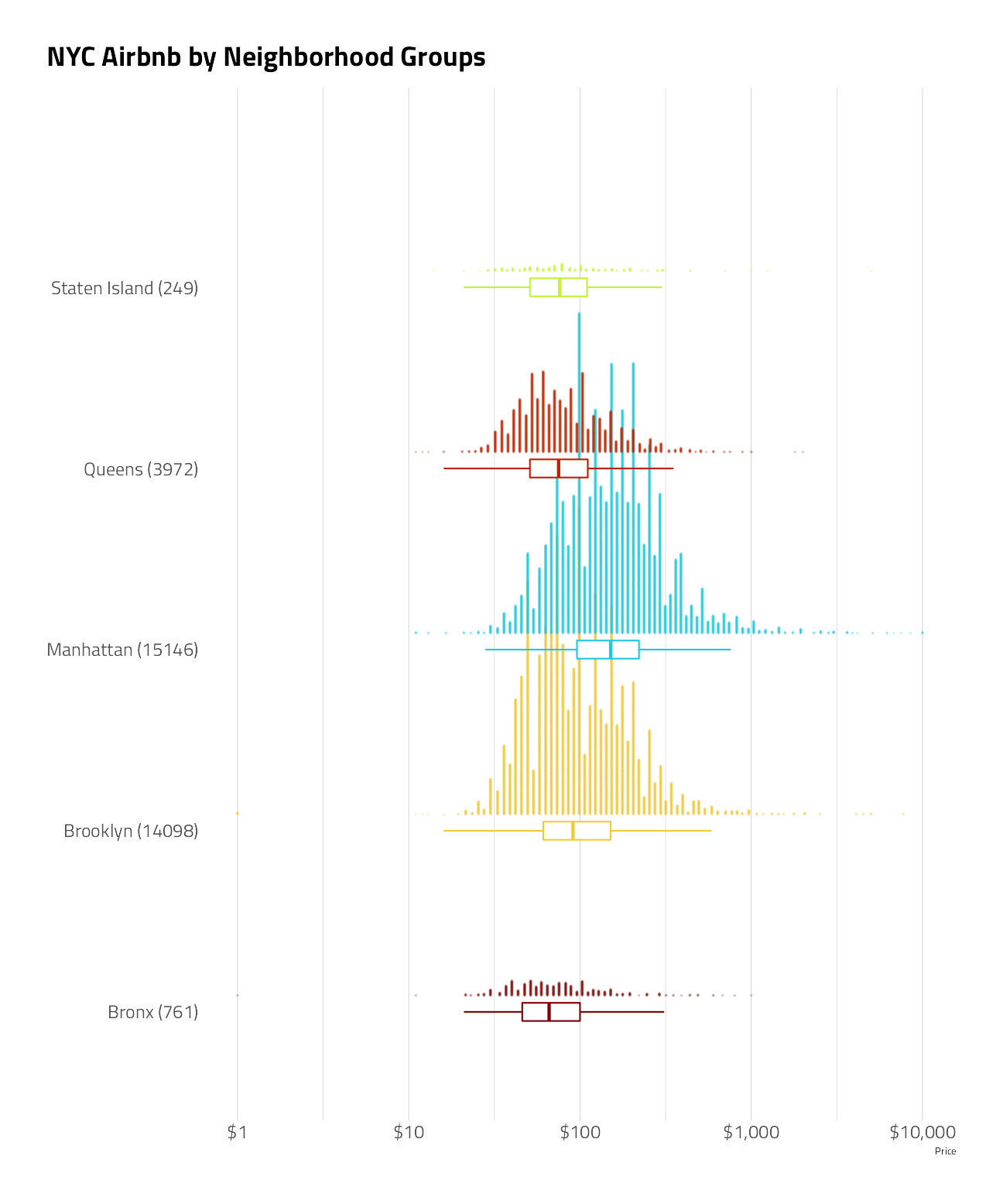

train_df %>%
  mutate(
    host_id = fct_lump(host_id, 30),
    host_id = fct_reorder(host_id, price)
  ) %>%
  group_by(host_id = withfreq(host_id)) %>%
  ggplot(aes(10^price, host_id)) +
  geom_boxplot(show.legend = FALSE) +
  scale_x_log10(labels = scales::dollar_format(accuracy = 1)) +
  labs(y = NULL, x = "Price", title = "NYC Airbnb by Host IDs")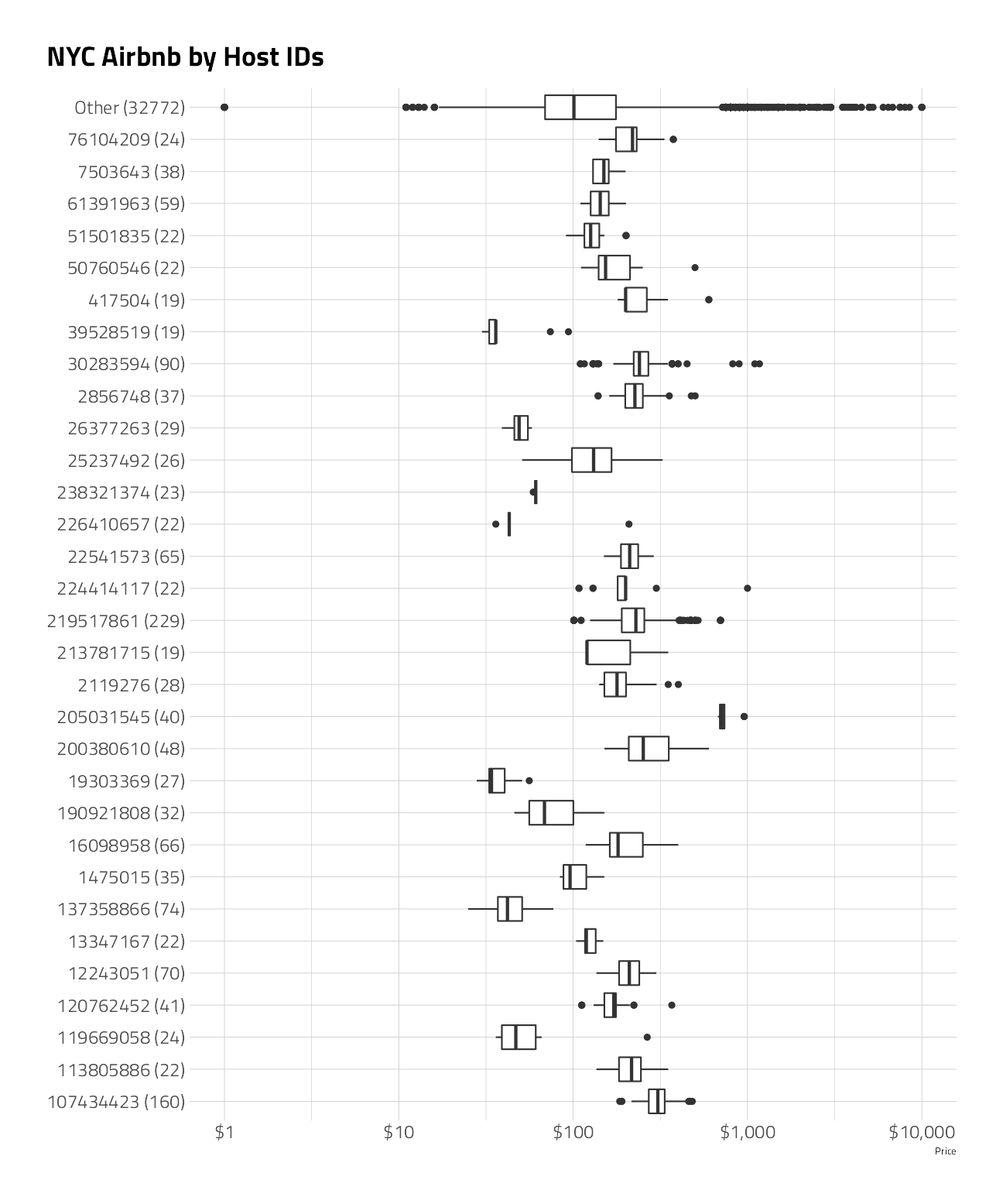

train_df %>%
  mutate(room_type = fct_reorder(room_type, price)) %>%
  group_by(room_type) %>%
  ggplot(aes(10^price,
    room_type,
    color = room_type
  )) +
  ggdist::stat_dots(
    aes(fill = room_type),
    side = "top",
    alpha = 0.2,
    justification = -0.1,
    binwidth = 0.03,
    dotsize = .5,
    stackratio = .08,
    normalize = "groups",
    show.legend = FALSE
  ) +
  geom_boxplot(
    width = 0.1,
    outlier.shape = NA,
    show.legend = FALSE
  ) +
  scale_x_log10(labels = scales::dollar_format(accuracy = 1)) +
  labs(y = NULL, x = "Price", title = "NYC Airbnb by Room Type")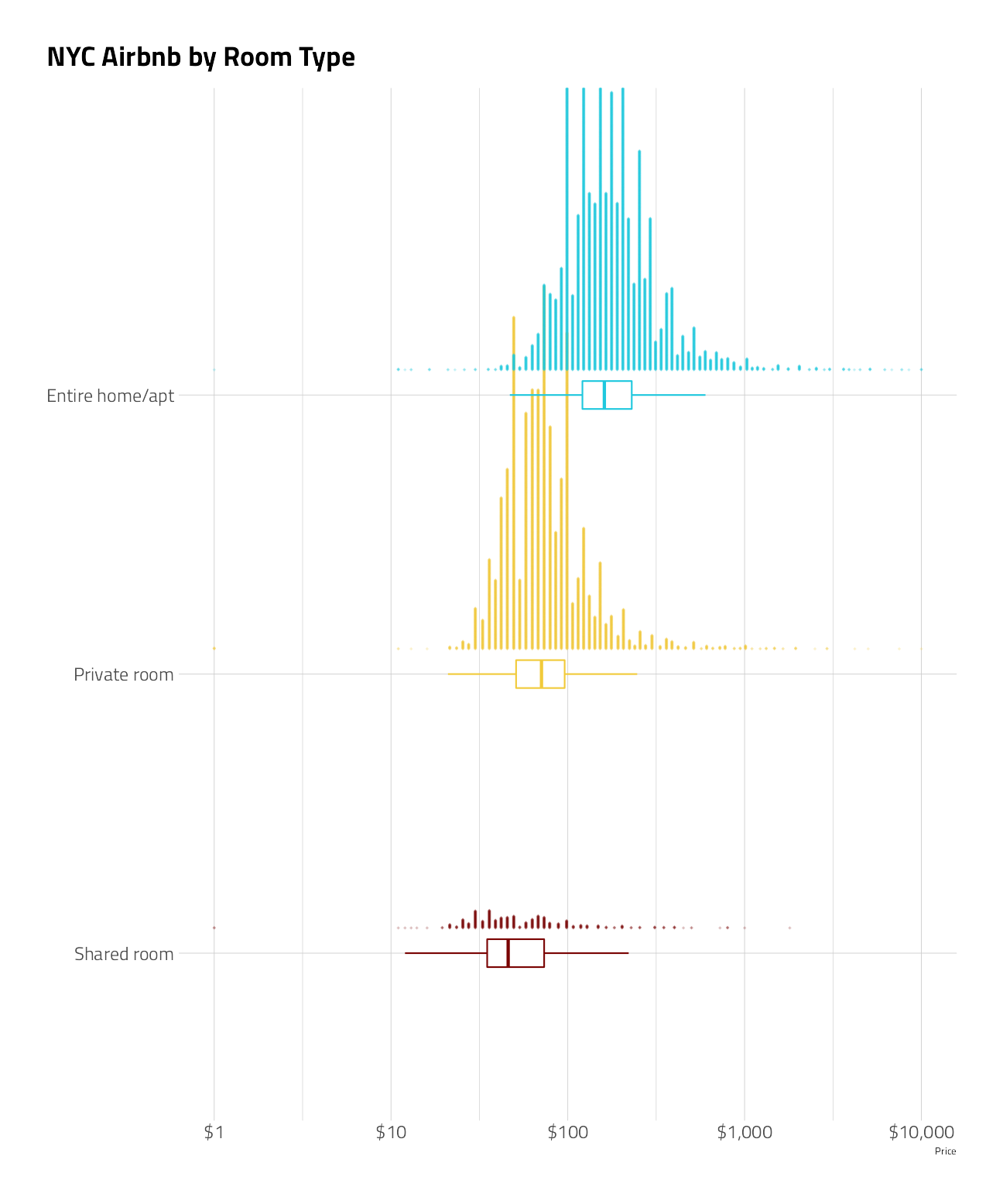

train_df %>%
  unnest_tokens(word, name) %>%
  anti_join(stop_words) %>%
  group_by(word) %>%
  summarize_prices() %>%
  head(30) %>%
  mutate(word = fct_reorder(word, mean_price)) %>%
  ggplot(aes(mean_price, word, size = n)) +
  geom_point() +
  scale_x_log10(labels = scales::dollar_format(accuracy = 1)) +
  labs(size = "Number of Listings", title = "NYC AirBNB Property Description NLP", y = NULL) +
  theme(
    legend.position = c(0.8, 0.3),
    legend.background = element_rect(color = "white")
  )

train_df %>%
  group_by(neighbourhood) %>%
  summarize_prices() %>%
  arrange(-median_price)

Numeric Feature Plots

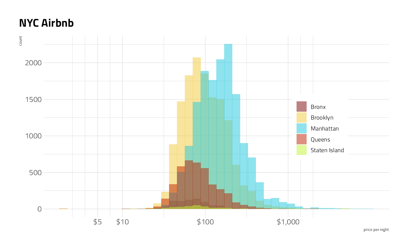
The outcome variable itself is skewed across all observations in the training data, as prices often are.

train_df %>%
  ggplot(aes(10^price + 1, fill = neighbourhood_group)) +
  geom_histogram(
    position = "identity",
    alpha = 0.5,
    bins = 40
  ) +
  scale_x_log10(
    labels = scales::dollar_format(accuracy = 1),
    breaks = c(5, 10, 100, 1000)
  ) +
  labs(
    fill = NULL, x = "price per night",
    title = "NYC Airbnb"
  ) +
  theme(
    legend.position = c(0.8, 0.5),
    legend.background = element_rect(color = "white")
  )

Let’s explore the relationships between the features and the numeric outcome.

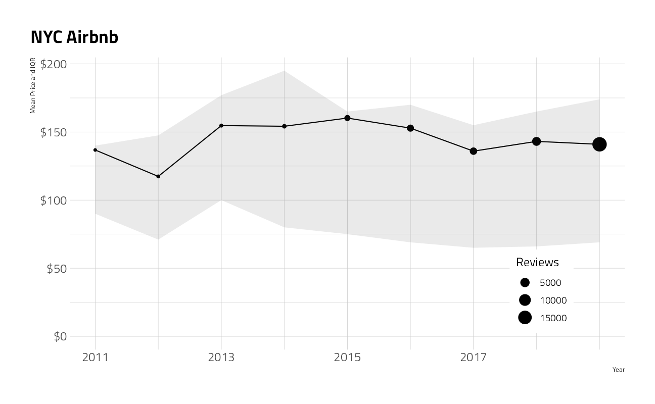
A plot of the time series last_review by year and the corresponding ranges of price

train_df %>%
  group_by(year = year(last_review)) %>%
  summarize(
    mean_price = mean(10^price - 1),
    n = n(),
    low = quantile(10^price - 1, probs = 0.25, na.rm = TRUE),
    high = quantile(10^price - 1, probs = 0.75, na.rm = TRUE),
    .groups = "drop"
  ) %>%
  filter(!is.na(year)) %>%
  ggplot(aes(year, mean_price)) +
  geom_line() +
  geom_point(aes(size = n)) +
  geom_ribbon(aes(ymin = low, ymax = high), alpha = .1) +
  expand_limits(y = 0) +
  scale_x_continuous(breaks = seq(2011, 2017, 2)) +
  scale_y_continuous(labels = scales::dollar_format(accuracy = 1)) +
  labs(
    x = "Year", y = "Mean Price and IQR",
    size = "Reviews", title = "NYC Airbnb"
  ) +
  theme(
    legend.position = c(0.85, 0.2),
    legend.background = element_rect(color = "white")
  )

Histograms of the distributions of each numeric feature:

train_numeric <- train_df %>%
  keep(is.numeric) %>%
  colnames()

chart <- c(train_numeric)

train_df %>%
  select_at(vars(all_of(chart))) %>%
  select(-price) %>%
  pivot_longer(
    cols = everything(),
    names_to = "key",
    values_to = "value"
  ) %>%
  filter(!is.na(value)) %>%
  ggplot() +
  geom_histogram(
    mapping = aes(x = value, fill = key),
    bins = 50, show.legend = FALSE
  ) +
  facet_wrap(~key, scales = "free", ncol = 3) +
  labs(title = "NYC Airbnb Numeric Feature Histograms")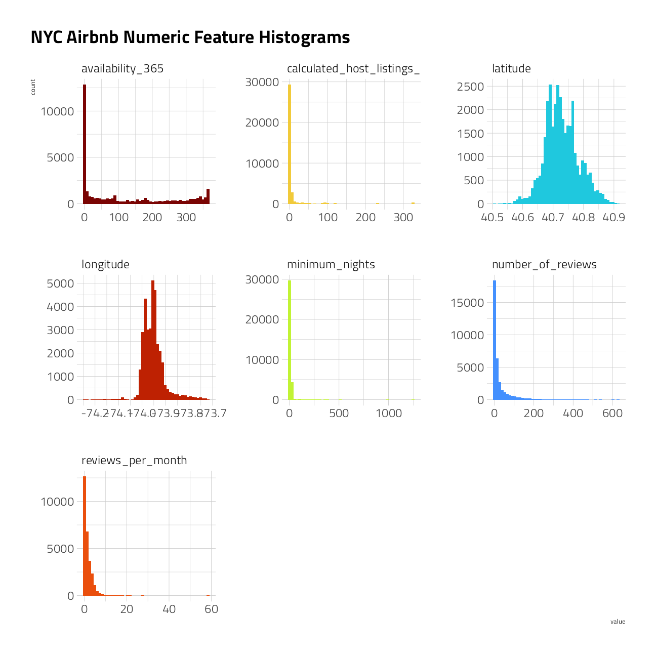

And the outcome variable by each numeric feature:

train_df %>%
  select_at(vars(all_of(chart))) %>%
  pivot_longer(
    cols = -price,
    names_to = "key",
    values_to = "value"
  ) %>%
  filter(!is.na(value)) %>%
  ggplot() +
  geom_point(
    mapping = aes(x = value, y = 10^price + 1),
    alpha = 0.1,
    shape = 20,
    show.legend = FALSE
  ) +
  geom_smooth(aes(
    x = value,
    y = 10^price + 1,
    color = key
  ),
  method = "gam", show.legend = FALSE
  ) +
  facet_wrap(~key, scales = "free", ncol = 3) +
  scale_y_log10(labels = scales::dollar_format(accuracy = 1)) +
  labs(x = NULL, y = "Price", title = "NYC Airbnb")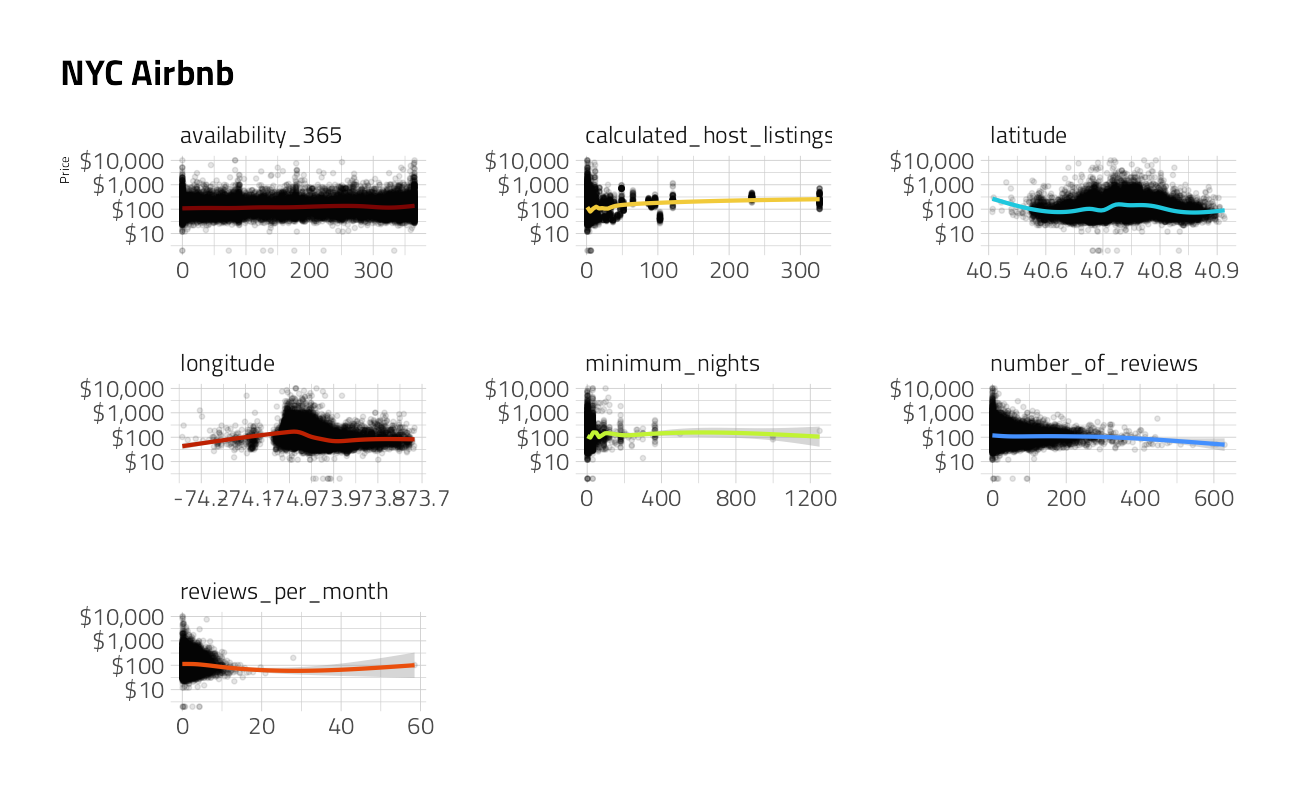

Map of prices

Adapted from Julia Silge’s demonstration

usa_data <- map_data("usa")

train_df %>%
  ggplot(aes(longitude, latitude, z = price)) +
  stat_summary_hex(bins = 100) +
  labs(fill = "Mean price(log10)") +
  cowplot::theme_map() +
  labs(title = "NYC Airbnb Price Ranges")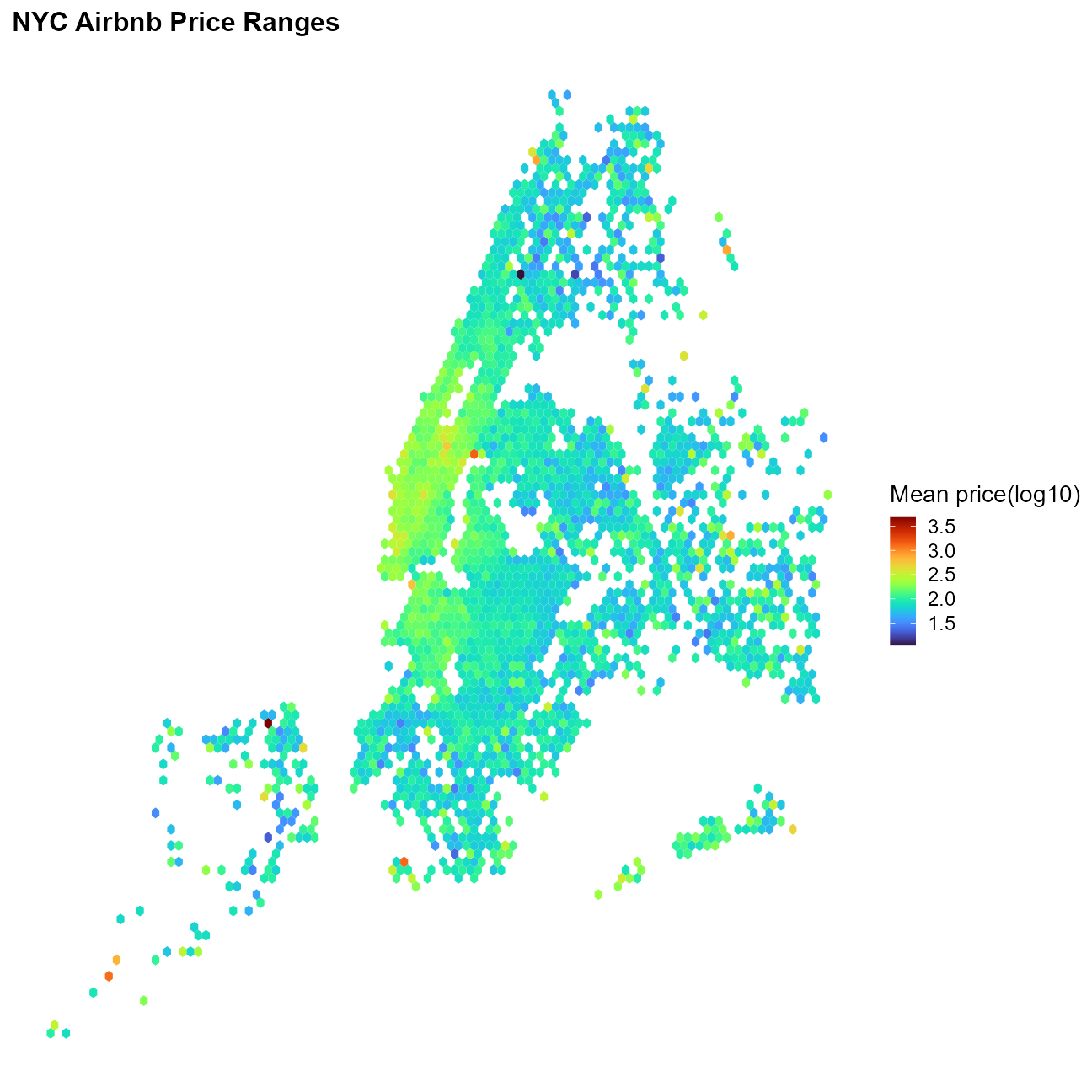

theme(
  legend.position = c(0.1, 0.8),
  legend.background = element_rect(color = "white")
)

List of 2
 $ legend.background:List of 5
  ..$ fill         : NULL
  ..$ colour       : chr "white"
  ..$ size         : NULL
  ..$ linetype     : NULL
  ..$ inherit.blank: logi FALSE
  ..- attr(*, "class")= chr [1:2] "element_rect" "element"
 $ legend.position  : num [1:2] 0.1 0.8
 - attr(*, "class")= chr [1:2] "theme" "gg"
 - attr(*, "complete")= logi FALSE
 - attr(*, "validate")= logi TRUE

Numeric Feature Correlations

cr1 <- train_df %>%
  select(-price) %>%
  keep(is.numeric) %>%
  cor(use = "pair")

corrplot::corrplot(cr1, type = "upper")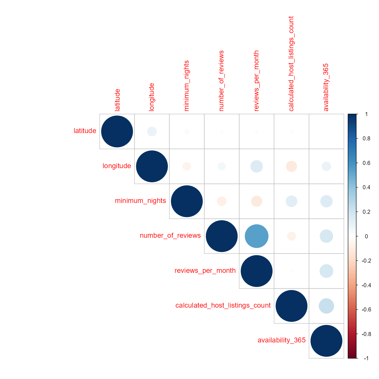

Conclusions:

• Neighborhood location drives price, through both named neighborhood and through longitude and latitude.
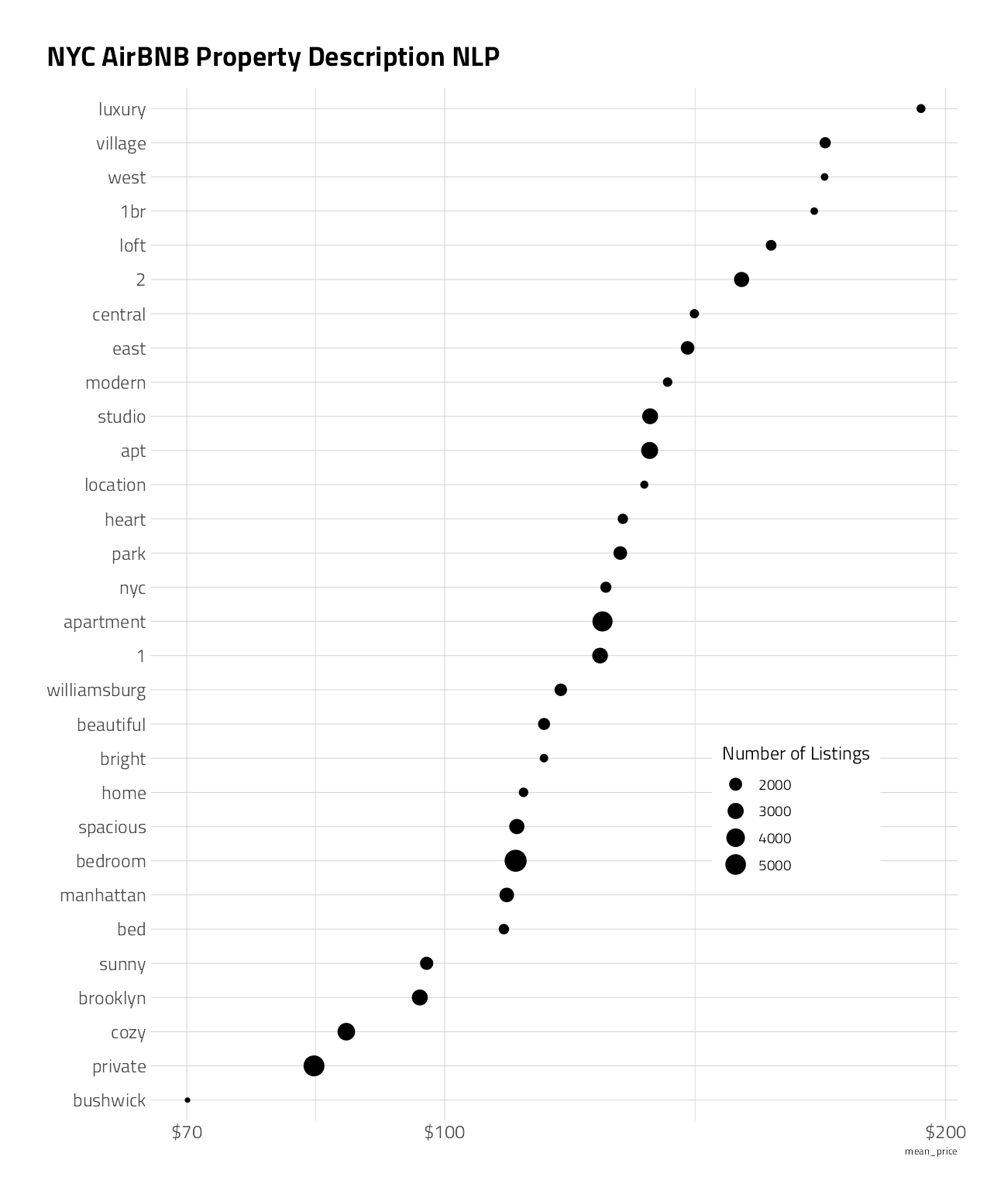
• The listing names have some interesting words.
• Some of the hosts draw higher pricing.
• the numeric features do not provide as much predictive power alone
• there are AirBNB listings that have neither reviews nor last_review dates.

Preprocessiong

The recipe framework

I am going to train on almost all of the train data. The 1% left is a quick confirmation of validity. The provided file labeled test has no labels.

set.seed(2021)
split <- train_df %>%
  initial_split(
    strata = price,
    prop = .99
  )
train <- training(split)
valid <- testing(split)

There are only 344 held out from training as a last check before submission.

basic_rec <-
  recipe(price ~ ., train) %>%
  # ---- set aside the row id's
  update_role(id, host_name, new_role = "id") %>%
  step_novel(neighbourhood) %>%
  step_other(neighbourhood, threshold = 0.01) %>%
  step_novel(host_id) %>%
  step_other(host_id, threshold = 0.01) %>%
  step_tokenize(name) %>%
  step_stopwords(name) %>%
  step_texthash(name, num_terms = 16) %>%
  step_indicate_na(last_review, reviews_per_month) %>%
  step_mutate(last_review = if_else(is.na(last_review),
    min(train$last_review, na.rm = TRUE), last_review
  )) %>%
  step_holiday(last_review) %>%
  step_date(last_review,
    features = "year",
    keep_original_cols = FALSE
  ) %>%
  step_ns(longitude, latitude, deg_free = 4) %>%
  step_normalize(all_numeric_predictors()) %>%
  step_nzv(all_predictors())

the pre-processed data

basic_rec %>%
  #  finalize_recipe(list(num_comp = 2)) %>%
  prep() %>%
  juice()

Cross Validation

We will use 5-fold cross validation and stratify between the rain and no-rain classes.

train_folds <- vfold_cv(
  data = train,
  strata = price,
  v = 5
)

Machine Learning

Model Specifications

We will build a specification for simple shallow random forest and a specification for catboost.

catboost_spec <- boost_tree(
  trees = 1000,
  min_n = tune(),
  learn_rate = tune(),
  tree_depth = tune()
) %>%
  set_engine("catboost") %>%
  set_mode("regression")

bag_spec <-
  bag_tree(min_n = 10) %>%
  set_engine("rpart", times = 50) %>%
  set_mode("regression")

The RMSLE custom metric

The yardstick default RMSE is on the log of price, not RMSLE on price. This will create a custom function to track RMSLE:

library(rlang)

rmsle_vec <- function(truth, estimate, na_rm = TRUE, ...) {
  rmsle_impl <- function(truth, estimate) {
    sqrt(mean((log(truth + 1) - log(estimate + 1))^2))
  }

  metric_vec_template(
    metric_impl = rmsle_impl,
    truth = truth,
    estimate = estimate,
    na_rm = na_rm,
    cls = "numeric",
    ...
  )
}

rmsle <- function(data, ...) {
  UseMethod("rmsle")
}

rmsle <- new_numeric_metric(rmsle, direction = "minimize")

rmsle.data.frame <- function(data, truth, estimate, na_rm = TRUE, ...) {
  metric_summarizer(
    metric_nm = "rmsle",
    metric_fn = rmsle_vec,
    data = data,
    truth = !!enquo(truth),
    estimate = !!enquo(estimate),
    na_rm = na_rm,
    ...
  )
}

mset <- metric_set(rmsle)

Parallel backend

To speed up computation we will use a parallel backend.

all_cores <- parallelly::availableCores(omit = 1)
all_cores

system 
    11 

future::plan("multisession", workers = all_cores) # on Windows

A quick Random Forest

Lets make a cursory check of the recipe and variable importance, which comes out of rpart for free. This workflow also handles factors without dummies.

bag_wf <-
  workflow() %>%
  add_recipe(basic_rec) %>%
  add_model(bag_spec)

set.seed(123)
bag_fit <- parsnip::fit(bag_wf, data = train)

extract_fit_parsnip(bag_fit)$fit$imp %>%
  mutate(term = fct_reorder(term, value)) %>%
  ggplot(aes(value, term)) +
  geom_point() +
  geom_errorbarh(aes(
    xmin = value - `std.error` / 2,
    xmax = value + `std.error` / 2
  ),
  height = .3
  ) +
  labs(
    title = "Feature Importance",
    x = NULL, y = NULL
  )

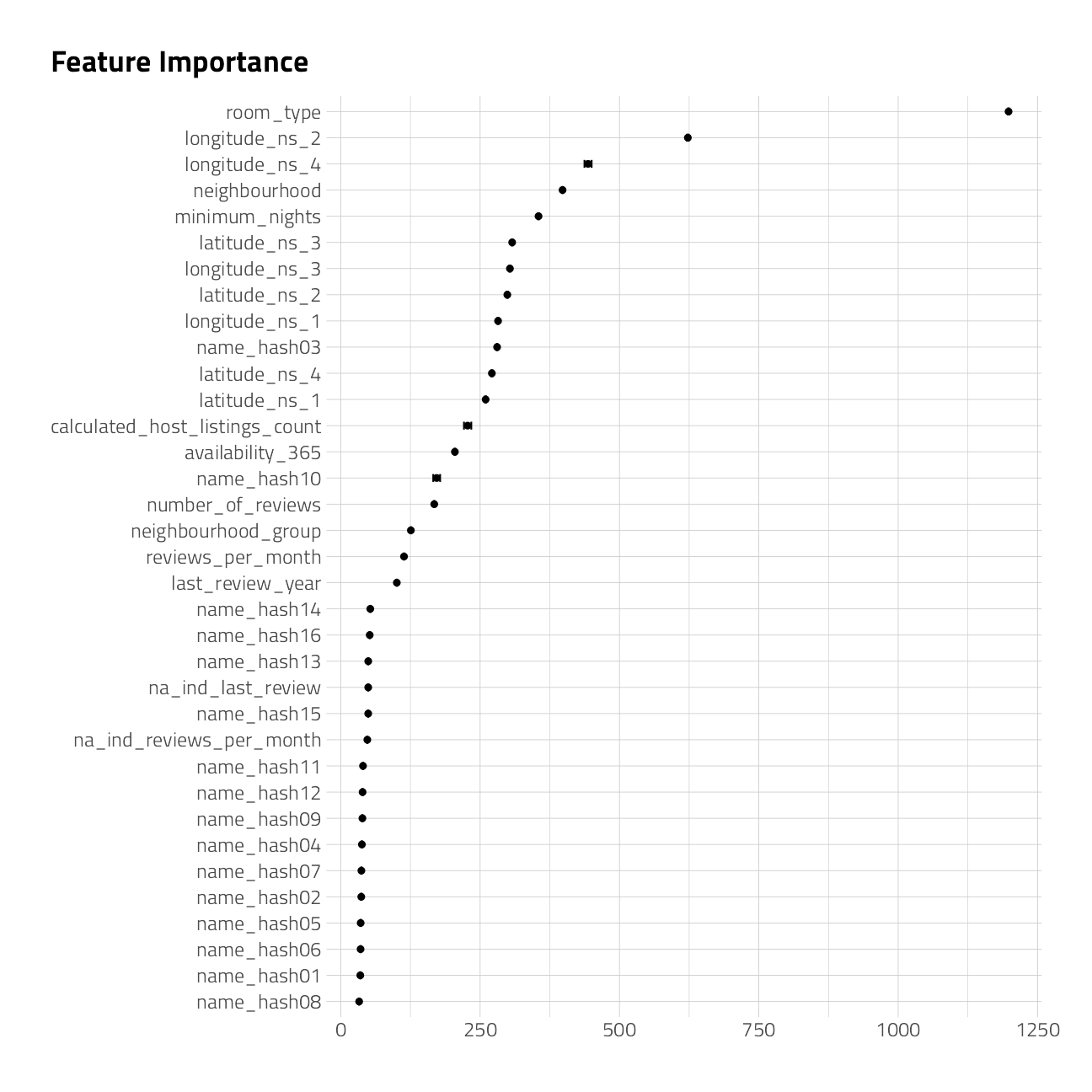
We see that room_type and the geographical information will be very important for this model.

Tuning Catboost

Now that we have some confidence that the features have predictive power, lets tune up a set of catboost models.

catboost_params <-
  dials::parameters(
    min_n(), # min data in leaf
    tree_depth(range = c(4, 15)),
    learn_rate(
      range = c(-3, -0.7),
      trans = log10_trans()
    )
  )

cbst_grid <- dials::grid_max_entropy(catboost_params,
  size = 40
)
cbst_grid

cv_res_catboost <-
  workflow() %>%
  add_recipe(basic_rec) %>%
  add_model(catboost_spec) %>%
  tune_grid(
    resamples = train_folds,
    grid = cbst_grid,
    control = control_race(
      verbose = FALSE,
      save_pred = TRUE,
      save_workflow = TRUE,
      extract = extract_model,
      parallel_over = "resamples"
    ),
    metrics = mset
  )

autoplot(cv_res_catboost)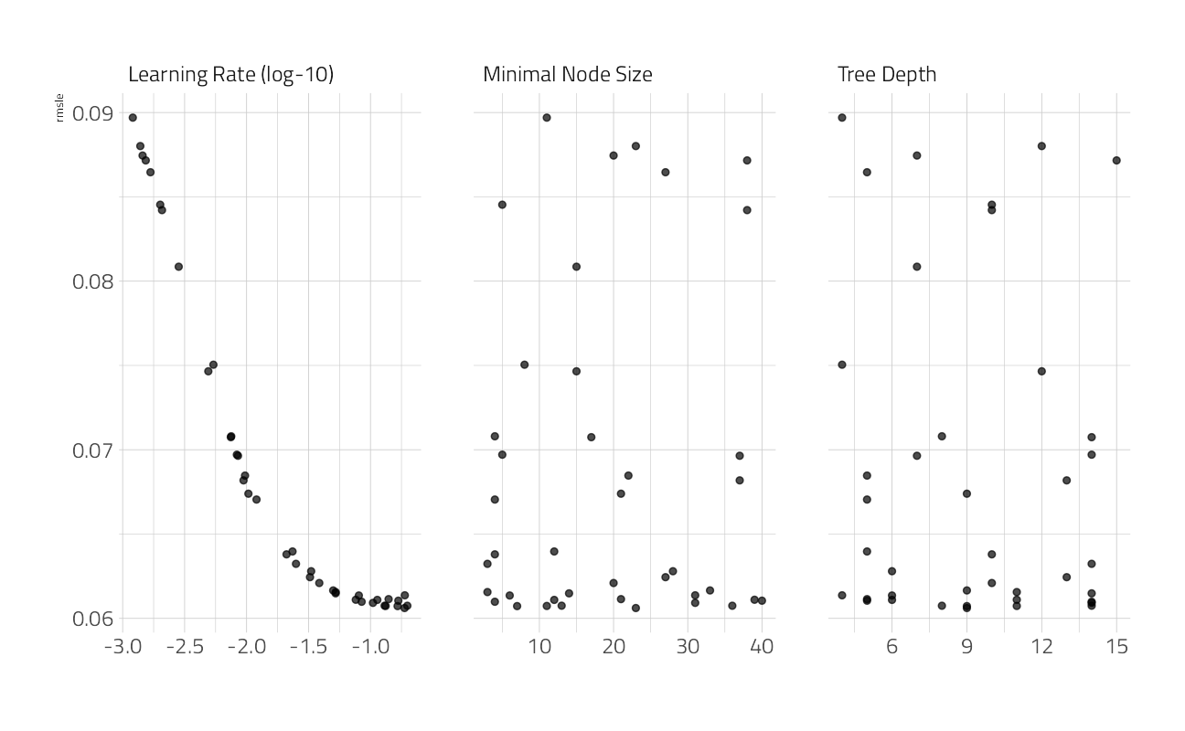

show_best(cv_res_catboost) %>%
  select(-.estimator)

cat_wf_best <-
  workflow() %>%
  add_recipe(basic_rec) %>%
  add_model(catboost_spec) %>%
  finalize_workflow(select_best(cv_res_catboost))

cat_fit_best <- cat_wf_best %>%
  parsnip::fit(data = train)

Catboost model performance

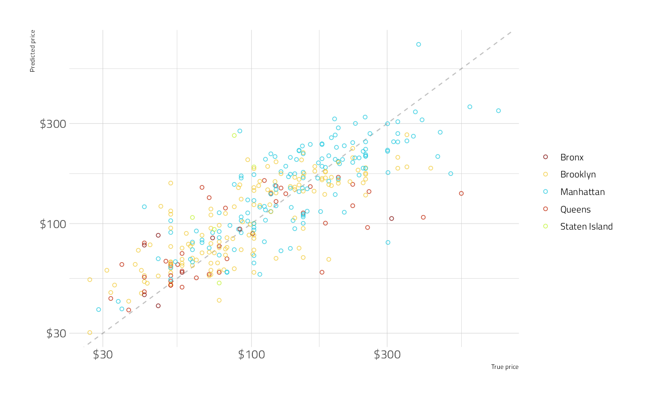
predict(cat_fit_best, new_data = valid) %>%
  cbind(valid) %>%
  ggplot(aes(10^price + 1,
    10^.pred + 1,
    color = neighbourhood_group
  )) +
  geom_abline(
    slope = 1,
    lty = 2,
    color = "gray50",
    alpha = 0.5
  ) +
  geom_point(alpha = 0.8, shape = 21) +
  scale_x_log10(labels = scales::dollar_format(accuracy = 1)) +
  scale_y_log10(labels = scales::dollar_format(accuracy = 1)) +
  labs(
    color = NULL,
    x = "True price",
    y = "Predicted price"
  )

predict(cat_fit_best, new_data = valid) %>%
  cbind(valid) %>%
  rmsle(10^price - 1, 10^.pred - 1)

This catboost figure is somewhat better than the leaderboard RMSLE of 0.40758, so it would have been worthy of submission.

Lastly, we build the submission file

bind_cols(predict(cat_fit_best, test_df), test_df) %>%
  select(id, price = .pred) %>%
  write_csv(file = path_export)

and make the submission to the Kaggle board

shell(glue::glue('kaggle competitions submit -c { competition_name } -f { path_export } -m "Catboosted"'))

Session information

sessionInfo()

R version 4.1.1 (2021-08-10)
Platform: x86_64-w64-mingw32/x64 (64-bit)
Running under: Windows 10 x64 (build 22000)

Matrix products: default

locale:
[1] LC_COLLATE=English_United States.1252 
[2] LC_CTYPE=English_United States.1252   
[3] LC_MONETARY=English_United States.1252
[4] LC_NUMERIC=C                          
[5] LC_TIME=English_United States.1252    

attached base packages:
[1] stats     graphics  grDevices utils     datasets  methods   base     

other attached packages:
 [1] rlang_0.4.11        catboost_0.26       baguette_0.1.1     
 [4] themis_0.1.4        stacks_0.2.1        finetune_0.1.0     
 [7] treesnip_0.1.0.9000 textrecipes_0.4.1   yardstick_0.0.8    
[10] workflowsets_0.1.0  workflows_0.2.3     tune_0.1.6         
[13] rsample_0.1.0       recipes_0.1.17      parsnip_0.1.7.900  
[16] modeldata_0.1.1     infer_1.0.0         dials_0.0.10       
[19] scales_1.1.1        broom_0.7.9         tidymodels_0.1.4   
[22] tidytext_0.3.2      lubridate_1.7.10    hrbrthemes_0.8.0   
[25] forcats_0.5.1       stringr_1.4.0       dplyr_1.0.7        
[28] purrr_0.3.4         readr_2.0.2         tidyr_1.1.4        
[31] tibble_3.1.4        ggplot2_3.3.5       tidyverse_1.3.1    
[34] workflowr_1.6.2    

loaded via a namespace (and not attached):
  [1] utf8_1.2.2           R.utils_2.11.0       tidyselect_1.1.1    
  [4] grid_4.1.1           pROC_1.18.0          munsell_0.5.0       
  [7] codetools_0.2-18     ragg_1.1.3           future_1.22.1       
 [10] withr_2.4.2          colorspace_2.0-2     highr_0.9           
 [13] knitr_1.36           rstudioapi_0.13      Rttf2pt1_1.3.8      
 [16] listenv_0.8.0        labeling_0.4.2       git2r_0.28.0        
 [19] TeachingDemos_2.12   lgr_0.4.3            farver_2.1.0        
 [22] bit64_4.0.5          DiceDesign_1.9       rprojroot_2.0.2     
 [25] mlr_2.19.0           parallelly_1.28.1    vctrs_0.3.8         
 [28] generics_0.1.0       float_0.2-6          ipred_0.9-12        
 [31] xfun_0.26            R6_2.5.1             doParallel_1.0.16   
 [34] lhs_1.1.3            cachem_1.0.6         assertthat_0.2.1    
 [37] vroom_1.5.5          promises_1.2.0.1     nnet_7.3-16         
 [40] gtable_0.3.0         Cubist_0.3.0         globals_0.14.0      
 [43] timeDate_3043.102    BBmisc_1.11          systemfonts_1.0.2   
 [46] text2vec_0.6         splines_4.1.1        extrafontdb_1.0     
 [49] butcher_0.1.5        stopwords_2.2        hexbin_1.28.2       
 [52] earth_5.3.1          checkmate_2.0.0      yaml_2.2.1          
 [55] reshape2_1.4.4       modelr_0.1.8         backports_1.2.1     
 [58] httpuv_1.6.3         tokenizers_0.2.1     extrafont_0.17      
 [61] inum_1.0-4           tools_4.1.1          lava_1.6.10         
 [64] usethis_2.0.1        ellipsis_0.3.2       jquerylib_0.1.4     
 [67] Rcpp_1.0.7           plyr_1.8.6           parallelMap_1.5.1   
 [70] rpart_4.1-15         ParamHelpers_1.14    viridis_0.6.1       
 [73] cowplot_1.1.1        haven_2.4.3          fs_1.5.0            
 [76] here_1.0.1           furrr_0.2.3          unbalanced_2.0      
 [79] magrittr_2.0.1       data.table_1.14.2    ggdist_3.0.0        
 [82] reprex_2.0.1         RANN_2.6.1           GPfit_1.0-8         
 [85] mlapi_0.1.0          mvtnorm_1.1-2        SnowballC_0.7.0     
 [88] whisker_0.4          ROSE_0.0-4           R.cache_0.15.0      
 [91] hms_1.1.1            evaluate_0.14        RhpcBLASctl_0.21-247
 [94] readxl_1.3.1         gridExtra_2.3        compiler_4.1.1      
 [97] maps_3.4.0           crayon_1.4.1         R.oo_1.24.0         
[100] htmltools_0.5.2      mgcv_1.8-36          later_1.3.0         
[103] tzdb_0.1.2           Formula_1.2-4        libcoin_1.0-9       
[106] DBI_1.1.1            corrplot_0.90        dbplyr_2.1.1        
[109] MASS_7.3-54          Matrix_1.3-4         cli_3.0.1           
[112] C50_0.1.5            R.methodsS3_1.8.1    parallel_4.1.1      
[115] gower_0.2.2          pkgconfig_2.0.3      rsparse_0.4.0       
[118] xml2_1.3.2           foreach_1.5.1        bslib_0.3.0         
[121] hardhat_0.1.6        plotmo_3.6.1         prodlim_2019.11.13  
[124] rvest_1.0.1          distributional_0.2.2 janeaustenr_0.1.5   
[127] digest_0.6.28        rmarkdown_2.11       cellranger_1.1.0    
[130] fastmatch_1.1-3      gdtools_0.2.3        nlme_3.1-152        
[133] lifecycle_1.0.1      jsonlite_1.7.2       viridisLite_0.4.0   
[136] fansi_0.5.0          pillar_1.6.3         lattice_0.20-44     
[139] fastmap_1.1.0        httr_1.4.2           plotrix_3.8-2       
[142] survival_3.2-11      glue_1.4.2           conflicted_1.0.4    
[145] FNN_1.1.3            iterators_1.0.13     bit_4.0.4           
[148] class_7.3-19         stringi_1.7.5        sass_0.4.0          
[151] rematch2_2.1.2       textshaping_0.3.5    partykit_1.2-15     
[154] styler_1.6.2         future.apply_1.8.1