European Flights

workflowr

• Summary
• Checks
• Past versions

Last updated: 2022-07-13

Checks: 7 0

Knit directory: myTidyTuesday/

This reproducible R Markdown analysis was created with workflowr (version 1.7.0). The Checks tab describes the reproducibility checks that were applied when the results were created. The Past versions tab lists the development history.

---

R Markdown file: up-to-date

Great! Since the R Markdown file has been committed to the Git repository, you know the exact version of the code that produced these results.

Environment: empty

Great job! The global environment was empty. Objects defined in the global environment can affect the analysis in your R Markdown file in unknown ways. For reproduciblity it’s best to always run the code in an empty environment.

Seed: set.seed(20210907)

The command set.seed(20210907) was run prior to running the code in the R Markdown file. Setting a seed ensures that any results that rely on randomness, e.g. subsampling or permutations, are reproducible.

Session information: recorded

Great job! Recording the operating system, R version, and package versions is critical for reproducibility.

Cache: none

Nice! There were no cached chunks for this analysis, so you can be confident that you successfully produced the results during this run.

File paths: relative

Great job! Using relative paths to the files within your workflowr project makes it easier to run your code on other machines.

Repository version: 773622d

Great! You are using Git for version control. Tracking code development and connecting the code version to the results is critical for reproducibility.

The results in this page were generated with repository version 773622d. See the Past versions tab to see a history of the changes made to the R Markdown and HTML files.

Note that you need to be careful to ensure that all relevant files for the analysis have been committed to Git prior to generating the results (you can use wflow_publish or wflow_git_commit). workflowr only checks the R Markdown file, but you know if there are other scripts or data files that it depends on. Below is the status of the Git repository when the results were generated:

Ignored files:
    Ignored:    .Rhistory
    Ignored:    .Rproj.user/
    Ignored:    data/.Rhistory
    Ignored:    data/CNHI_Excel_Chart.xlsx
    Ignored:    data/Chicago.rds
    Ignored:    data/CommunityTreemap.jpeg
    Ignored:    data/Community_Roles.jpeg
    Ignored:    data/SeriesReport-20220414171148_6c3b18.xlsx
    Ignored:    data/Weekly_Chicago_IL_Regular_Reformulated_Retail_Gasoline_Prices.csv
    Ignored:    data/YammerDigitalDataScienceMembership.xlsx
    Ignored:    data/YammerMemberPage.rds
    Ignored:    data/YammerMembers.rds
    Ignored:    data/df.rds
    Ignored:    data/grainstocks.rds
    Ignored:    data/hike_data.rds
    Ignored:    data/netflixTitles.rds
    Ignored:    data/netflixTitles2.rds
    Ignored:    data/raw_weather.RData
    Ignored:    data/us_states.rds
    Ignored:    data/us_states_hexgrid.geojson
    Ignored:    data/weatherstats_toronto_daily.csv

Untracked files:
    Untracked:  analysis/2022_May_tabular_playground.Rmd
    Untracked:  analysis/2022_May_tabular_playground_tabnet.Rmd
    Untracked:  code/YammerReach.R
    Untracked:  code/autokeras.R
    Untracked:  code/chicago.R
    Untracked:  code/glmnet_test.R
    Untracked:  code/googleCompute.R
    Untracked:  code/work list batch targets.R
    Untracked:  environment.yml
    Untracked:  figure/
    Untracked:  report.html

Unstaged changes:
    Modified:   analysis/2021_01_19_tidy_tuesday.Rmd
    Modified:   analysis/2021_03_24_tidy_tuesday.Rmd
    Deleted:    analysis/2021_04_20.Rmd
    Deleted:    analysis/2022_02_11_tabular_playground.Rmd
    Deleted:    analysis/2022_04_18.qmd
    Modified:   analysis/Survival.Rmd
    Modified:   analysis/_site.yml
    Modified:   code/_common.R

Note that any generated files, e.g. HTML, png, CSS, etc., are not included in this status report because it is ok for generated content to have uncommitted changes.

---

These are the previous versions of the repository in which changes were made to the R Markdown (analysis/2022_07_13_tidy_tuesday.Rmd) and HTML (docs/2022_07_13_tidy_tuesday.html) files. If you’ve configured a remote Git repository (see ?wflow_git_remote), click on the hyperlinks in the table below to view the files as they were in that past version.

File	Version	Author	Date	Message
Rmd	773622d	opus1993	2022-07-13	add geofacet and text sizing and
html	34a1569	opus1993	2022-07-13	Build site.
Rmd	33e29e5	opus1993	2022-07-13	add geofacet and text sizing and
html	9094d54	opus1993	2022-07-13	Build site.
Rmd	2d4ad41	opus1993	2022-07-13	add geofacet and text sizing
html	7396b5c	opus1993	2022-07-13	Build site.
Rmd	0e43049	opus1993	2022-07-13	add geofacet
html	c37dd08	opus1993	2022-07-13	Build site.
Rmd	dd63c3c	opus1993	2022-07-13	give credit to brendialj
html	1e824f6	opus1993	2022-07-13	Build site.
Rmd	cba7dfc	opus1993	2022-07-13	wflow_publish("analysis/2022_07_13_tidy_tuesday.Rmd")

---

In this weeks #TidyTuesday we take a look at the number of flights arriving and departing from several large European airports.

data is via Eurocontrol at https://ec.europa.eu/eurostat/web/products-eurostat-news/-/ddn-20210914-1

suppressPackageStartupMessages({
library(tidyverse)
library(lubridate)
library(patchwork)
  
library(geofacet)
 })

source(here::here("code","_common.R"),
       verbose = FALSE,
       local = knitr::knit_global())

ggplot2::theme_set(grumanlib::theme_jim(base_size = 12))

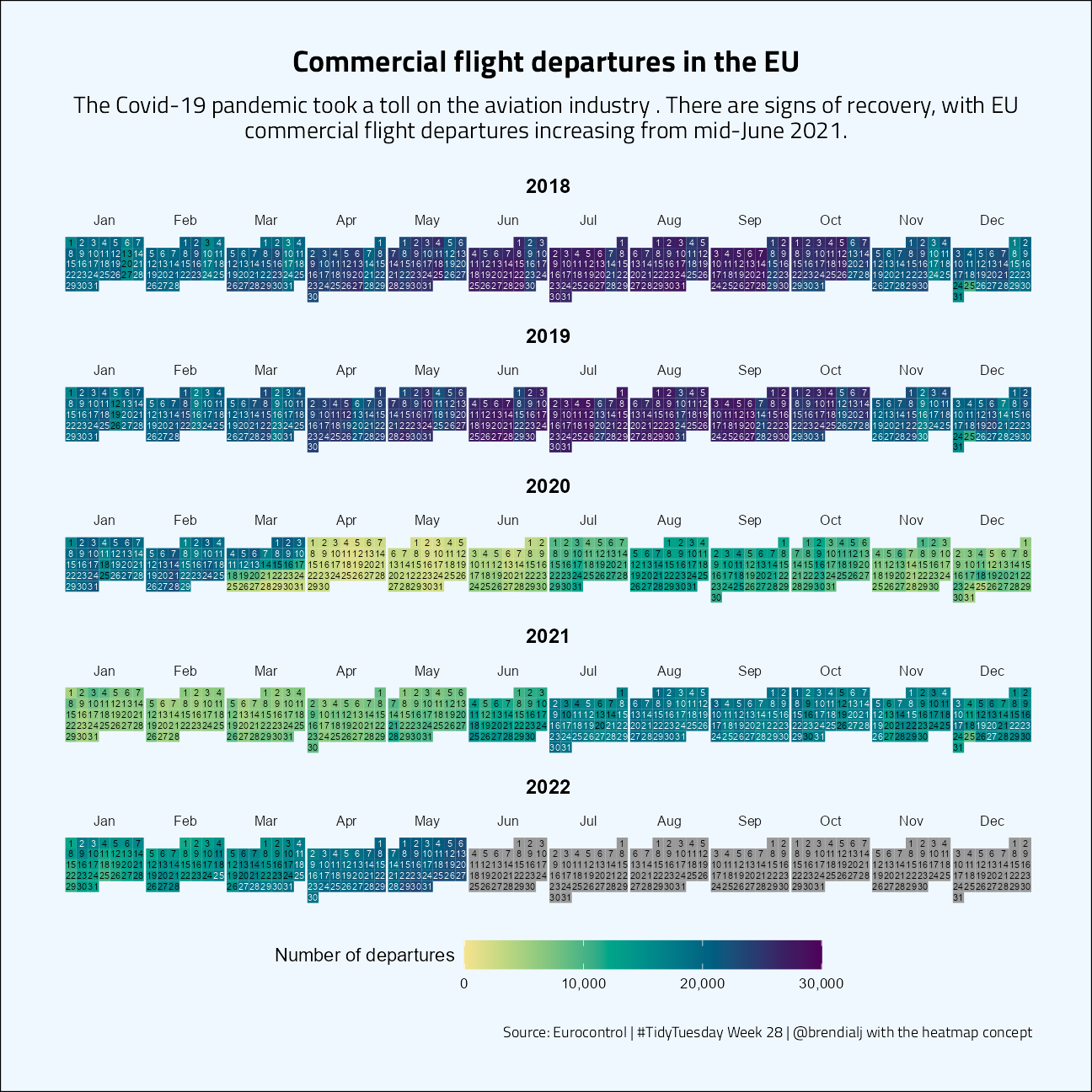
Let’s see what we can do to improve BrendiA’s heatmap:

tweetrmd::include_tweet("https://twitter.com/brendialj/status/1547206511910600706")

For this week's #TidyTuesday, I examined the total commercial flight departures across the EU. The recent months show signs of recovery for the aviation industry after the pandemic hit.#RStats code: https://t.co/2sIpKRS1Ur#dataviz #ggplot2 pic.twitter.com/LJO5m4el58

— Brendi Ang (@brendialj) July 13, 2022

tt <- tidytuesdayR::tt_load("2022-07-12")

    Downloading file 1 of 1: `flights.csv`

flights <- tt$flights |>
  rename(airport_label = `Pivot Label`) |>
  janitor::clean_names() |>
  select(-year, -month_num, -month_mon)

total_flights <- flights |>
  group_by(flt_date) |>
  summarise(
    total_dep = sum(flt_dep_1, na.rm = TRUE),
    .groups = "drop"
  ) |>
  complete(flt_date = seq.Date(
    from = as_date("2022-01-01"),
    to = as_date("2022-12-31"),
    by = "day",
    fill = list(value = NA)
  )) |>
  mutate(
    year = year(flt_date),
    week_of_year = week(flt_date),
    month = month(flt_date, label = TRUE, abbr = TRUE),
    day = day(flt_date)
  )

# Function prepares data for plotting based on a given year by BrendiA at https://github.com/BrendiA/tidy-tuesday/blob/main/2022/week-28/week-28.R
create_df <- function(given_year) {

  # Extract first day of the week for the year
  first_day_of_year <-
    wday(as_date(paste(given_year, "01", "01", sep = "-")),
      week_start = 1
    )

  total_flights |>
    filter(year == given_year) |>
    mutate(day_of_week = wday(flt_date,
      label = TRUE,
      week_start = first_day_of_year
    )) |>
    #    mutate(day_of_week = forcats::fct_rev(day_of_week)) |>
    group_by(month) |>
    mutate(week_of_month = -1 * dense_rank(week_of_year)) |>
    ungroup()
}

best_contrast <- function(x, y = c("#010101", "#FFFFFF")) {
  contrasts <- prismatic::contrast_ratio(x, y)
  y[max(contrasts) == contrasts][1]
}

# Function plots heatmap based on the data generated by BrendiA at https://github.com/BrendiA/tidy-tuesday/blob/main/2022/week-28/week-28.R  with Emil Hvitfeldt's Prismatic text color adjustments
plot_heatmap <- function(df) {

  # Year list of the data frame
  given_year <- unique(df$year)

  ggplot(
    data = df,
    aes(
      y = week_of_month,
      x = day_of_week,
      fill = total_dep
    )
  ) +
    # Heat map
    geom_tile() +
    # Calendar days
    geom_text(aes(
      label = day,
      color = ggplot2::after_scale(purrr::map_chr(fill, best_contrast))
    ),
    size = 2
    ) +
    colorspace::scale_fill_continuous_sequential(
      name = "Number of departures",
      palette = "Viridis",
      na.value = "grey60", # Fill missing dates
      limits = c(0, 30000),
      breaks = seq(0, 30000, 10000),
      oob = scales::squish,
      label = scales::label_comma(accuracy = 1),
      c2 = 60, # increase
      l1 = 10
    ) + # decrease
    facet_wrap(~month,
      nrow = 1
    ) +
    theme_minimal() +
    labs(title = given_year) +
    theme(
      axis.text.x = element_blank(),
      axis.text.y = element_blank(),
      axis.title = element_blank(),
      legend.direction = "horizontal",
      legend.key.width = unit(1.5, "cm"),
      legend.text = element_text(family = "Regular 400"),
      legend.title = element_text(vjust = 0.8, family = "Regular 400"),
      panel.spacing.x = unit(0, "lines"),
      panel.grid = element_blank(),
      plot.title = element_text(hjust = 0.5, family = "Black 900 Italic", size = 12, face = "bold"),
      strip.text = element_text(family = "Regular 400", size = 8)
    )
}

plot_list <-
  purrr::map(
    unique(sort(total_flights$year)),
    ~ create_df(.x) |>
      plot_heatmap()
  )

The functions above create a big list of heat maps, one for each year. I’ve added prismatic contrasts to the geom_text to make the dates just a bit more legible.

# Subtitle
sub <-
  str_wrap(
    "The Covid-19 pandemic took a toll on the aviation industry .
    There are signs of recovery, with EU commercial flight departures increasing from mid-June 2021.",
    width = 100
  )

plot_list[[3]] +
  plot_list[[4]] +
  plot_list[[5]] +
  plot_list[[6]] +
  plot_list[[7]] +
  plot_layout(
    guides = "collect",
    ncol = 1,
    height = 0.5
  ) &
  plot_annotation(
    title = "Commercial flight departures in the EU",
    subtitle = sub,
    caption = "Source: Eurocontrol | #TidyTuesday Week 28 | @brendialj with the heatmap concept",
    theme = theme(
      legend.position = "bottom",
      plot.title = element_text(hjust = 0.5, size = 18, face = "bold"),
      plot.subtitle = element_text(hjust = 0.5, size = 14),
      plot.background = element_rect(fill = "#f0f8ff"),
      plot.caption = element_text(vjust = 1)
    )
  )

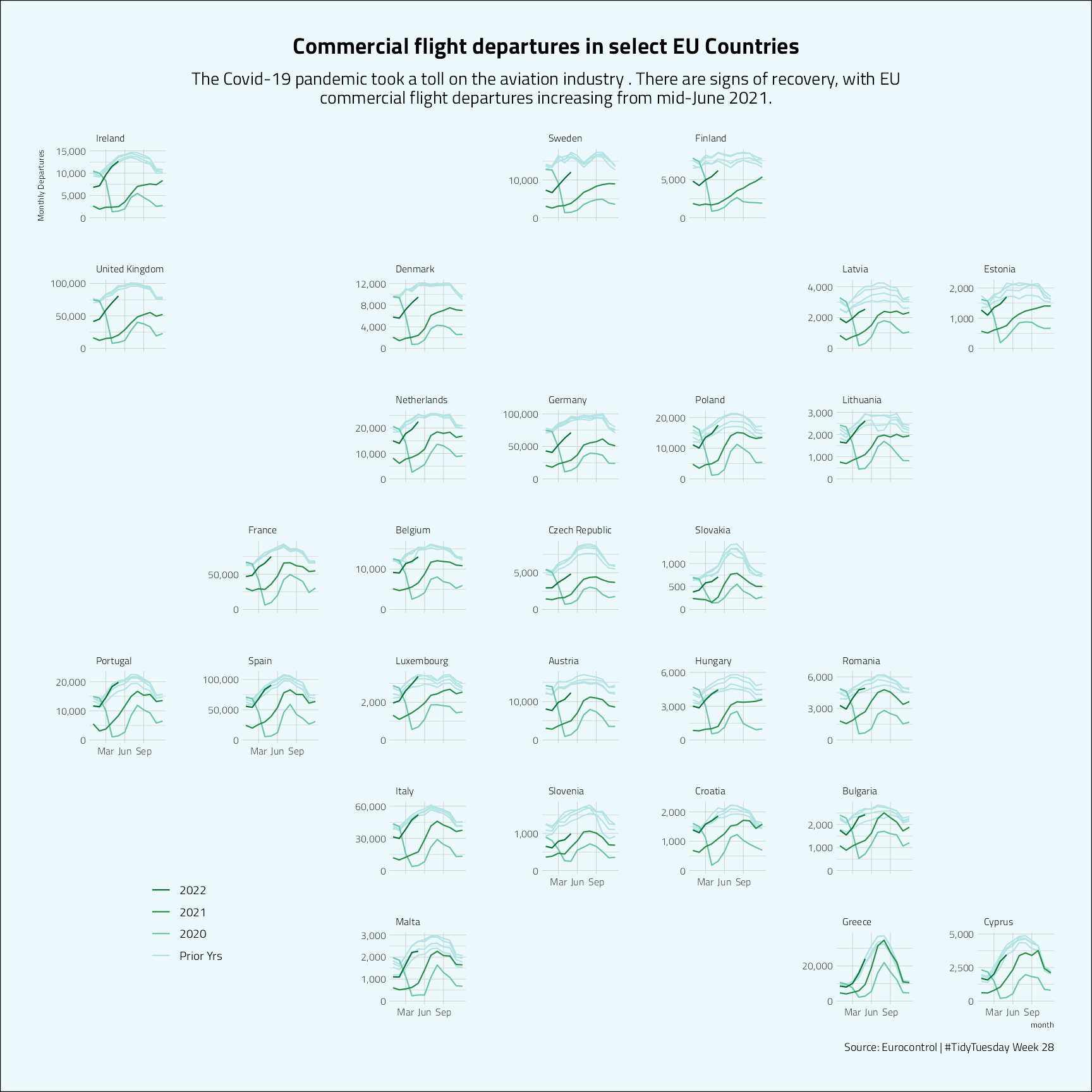
Cameron Kay posted a noteworthy animation. I’ll skip doing an animation this time go another direction.

tweetrmd::include_tweet("https://twitter.com/cameronskay/status/1547291272183832577")

My first #TidyTuesday contribution (now with legible text and more Norway!) #ICPSR #sumprog22 pic.twitter.com/efky0OQfLD

— Cameron Kay (@cameronskay) July 13, 2022

flights |>
  group_by(year = year(flt_date), month = month(flt_date), state_name) |>
  summarise(
    total_dep = sum(flt_dep_1, na.rm = TRUE),
    .groups = "drop"
  ) |>
  mutate(color = case_when(
    year < 2020 ~ "#b2e2e2",
    year == 2020 ~ "#66c2a4",
    year == 2021 ~ "#238b45",
    year == 2022 ~ "#006d2c"
  )) |>
  ggplot(aes(
    x = month,
    total_dep
  )) +
  geom_line(aes(
    group = factor(year),
    color = color
  ),
  show.legend = TRUE
  ) +
  scale_color_identity(
    guide = "legend",
    labels = c("2022", "2021", "2020", "Prior Yrs")
  ) +
  scale_x_continuous(
    breaks = c(3, 6, 9),
    labels = c("Mar", "Jun", "Sep"),
    minor_breaks = NULL
  ) +
  scale_y_continuous(
    limits = c(0, NA),
    n.breaks = 3,
    labels = scales::comma
  ) +
  facet_geo(~state_name,
    grid = "eu_grid1",
    label = "name",
    scales = "free_y"
  ) +
  labs(
    y = "Monthly Departures",
    title = "Commercial flight departures in select EU Countries",
    subtitle = sub,
    color = NULL,
    caption = "Source: Eurocontrol | #TidyTuesday Week 28"
  ) +
  theme(
    legend.position = c(0.1, 0.1),
    plot.title = element_text(hjust = 0.5, size = 18, face = "bold"),
    plot.subtitle = element_text(hjust = 0.5, size = 14),
    axis.text.x = element_text(size = 8),
    axis.text.y = element_text(size = 8),
    strip.text = element_text(size = 8),
    plot.background = element_rect(fill = "#edf8fb"),
    plot.caption = element_text(vjust = 1)
  )

Session information

sessionInfo()

R version 4.1.3 (2022-03-10)
Platform: x86_64-w64-mingw32/x64 (64-bit)
Running under: Windows 10 x64 (build 22000)

Matrix products: default

locale:
[1] LC_COLLATE=English_United States.1252 
[2] LC_CTYPE=English_United States.1252   
[3] LC_MONETARY=English_United States.1252
[4] LC_NUMERIC=C                          
[5] LC_TIME=English_United States.1252    

attached base packages:
[1] stats     graphics  grDevices utils     datasets  methods   base     

other attached packages:
 [1] geofacet_0.2.0  patchwork_1.1.1 lubridate_1.8.0 forcats_0.5.1  
 [5] stringr_1.4.0   dplyr_1.0.9     purrr_0.3.4     readr_2.1.2    
 [9] tidyr_1.2.0     tibble_3.1.7    ggplot2_3.3.6   tidyverse_1.3.1
[13] workflowr_1.7.0

loaded via a namespace (and not attached):
  [1] readxl_1.4.0         backports_1.4.1      systemfonts_1.0.4   
  [4] workflows_1.0.0      selectr_0.4-2        tidytuesdayR_1.0.2  
  [7] sp_1.5-0             splines_4.1.3        listenv_0.8.0       
 [10] usethis_2.1.6        digest_0.6.29        foreach_1.5.2       
 [13] htmltools_0.5.2      yardstick_1.0.0      viridis_0.6.2       
 [16] parsnip_1.0.0        fansi_1.0.3          magrittr_2.0.3      
 [19] memoise_2.0.1        tune_1.0.0           tzdb_0.3.0          
 [22] recipes_1.0.1        globals_0.15.1       modelr_0.1.8        
 [25] gower_1.0.0          vroom_1.5.7          R.utils_2.12.0      
 [28] hardhat_1.2.0        rsample_1.0.0        jpeg_0.1-9          
 [31] dials_1.0.0          colorspace_2.0-3     rvest_1.0.2         
 [34] ggrepel_0.9.1        textshaping_0.3.6    haven_2.5.0         
 [37] xfun_0.31            prismatic_1.1.0      callr_3.7.0         
 [40] crayon_1.5.1         jsonlite_1.8.0       survival_3.3-1      
 [43] iterators_1.0.14     glue_1.6.2           gtable_0.3.0        
 [46] ipred_0.9-13         R.cache_0.15.0       tweetrmd_0.0.9      
 [49] future.apply_1.9.0   imguR_1.0.3          scales_1.2.0        
 [52] infer_1.0.2          DBI_1.1.3            Rcpp_1.0.9          
 [55] viridisLite_0.4.0    units_0.8-0          bit_4.0.4           
 [58] GPfit_1.0-8          proxy_0.4-27         lava_1.6.10         
 [61] prodlim_2019.11.13   geogrid_0.1.1        httr_1.4.3          
 [64] ellipsis_0.3.2       farver_2.1.1         R.methodsS3_1.8.2   
 [67] pkgconfig_2.0.3      nnet_7.3-17          sass_0.4.1          
 [70] dbplyr_2.2.1         janitor_2.1.0        utf8_1.2.2          
 [73] here_1.0.1           labeling_0.4.2       tidyselect_1.1.2    
 [76] rlang_1.0.3          DiceDesign_1.9       later_1.3.0         
 [79] munsell_0.5.0        cellranger_1.1.0     tools_4.1.3         
 [82] cachem_1.0.6         cli_3.3.0            generics_0.1.3      
 [85] broom_1.0.0          evaluate_0.15        fastmap_1.1.0       
 [88] yaml_2.3.5           ragg_1.2.2           rematch2_2.1.2      
 [91] bit64_4.0.5          processx_3.7.0       knitr_1.39          
 [94] fs_1.5.2             workflowsets_0.2.1   future_1.26.1       
 [97] whisker_0.4          R.oo_1.25.0          xml2_1.3.3          
[100] compiler_4.1.3       rstudioapi_0.13      curl_4.3.2          
[103] png_0.1-7            e1071_1.7-11         reprex_2.0.1        
[106] lhs_1.1.5            bslib_0.3.1          stringi_1.7.8       
[109] highr_0.9            ps_1.7.1             rgeos_0.5-9         
[112] lattice_0.20-45      Matrix_1.4-0         styler_1.7.0        
[115] classInt_0.4-7       conflicted_1.1.0     vctrs_0.4.1         
[118] tidymodels_0.2.0     pillar_1.7.0         lifecycle_1.0.1     
[121] furrr_0.3.0          jquerylib_0.1.4      httpuv_1.6.5        
[124] R6_2.5.1             promises_1.2.0.1     KernSmooth_2.23-20  
[127] gridExtra_2.3        parallelly_1.32.0    codetools_0.2-18    
[130] MASS_7.3-55          assertthat_0.2.1     rprojroot_2.0.3     
[133] withr_2.5.0          rnaturalearth_0.1.0  parallel_4.1.3      
[136] hms_1.1.1            grid_4.1.3           rpart_4.1.16        
[139] timeDate_3043.102    class_7.3-20         snakecase_0.11.0    
[142] rmarkdown_2.14       grumanlib_0.1.0.9999 git2r_0.30.1        
[145] sf_1.0-7             getPass_0.2-2