Kaggle Feedback Prize - English Language Learning

workflowr

• Summary
• Checks
• Past versions

Last updated: 2022-10-15

Checks: 7 0

Knit directory: myTidyTuesday/

This reproducible R Markdown analysis was created with workflowr (version 1.7.0). The Checks tab describes the reproducibility checks that were applied when the results were created. The Past versions tab lists the development history.

---

R Markdown file: up-to-date

Great! Since the R Markdown file has been committed to the Git repository, you know the exact version of the code that produced these results.

Environment: empty

Great job! The global environment was empty. Objects defined in the global environment can affect the analysis in your R Markdown file in unknown ways. For reproduciblity it’s best to always run the code in an empty environment.

Seed: set.seed(20210907)

The command set.seed(20210907) was run prior to running the code in the R Markdown file. Setting a seed ensures that any results that rely on randomness, e.g. subsampling or permutations, are reproducible.

Session information: recorded

Great job! Recording the operating system, R version, and package versions is critical for reproducibility.

Cache: none

Nice! There were no cached chunks for this analysis, so you can be confident that you successfully produced the results during this run.

File paths: relative

Great job! Using relative paths to the files within your workflowr project makes it easier to run your code on other machines.

Repository version: 73c07de

Great! You are using Git for version control. Tracking code development and connecting the code version to the results is critical for reproducibility.

The results in this page were generated with repository version 73c07de. See the Past versions tab to see a history of the changes made to the R Markdown and HTML files.

Note that you need to be careful to ensure that all relevant files for the analysis have been committed to Git prior to generating the results (you can use wflow_publish or wflow_git_commit). workflowr only checks the R Markdown file, but you know if there are other scripts or data files that it depends on. Below is the status of the Git repository when the results were generated:

Ignored files:
    Ignored:    .Rhistory
    Ignored:    .Rproj.user/
    Ignored:    data/.Rhistory
    Ignored:    data/CNHI_Excel_Chart.xlsx
    Ignored:    data/Chicago.rds
    Ignored:    data/CommunityTreemap.jpeg
    Ignored:    data/Community_Roles.jpeg
    Ignored:    data/SeriesReport-20220414171148_6c3b18.xlsx
    Ignored:    data/Weekly_Chicago_IL_Regular_Reformulated_Retail_Gasoline_Prices.csv
    Ignored:    data/YammerDigitalDataScienceMembership.xlsx
    Ignored:    data/YammerMemberPage.rds
    Ignored:    data/YammerMembers.rds
    Ignored:    data/df.rds
    Ignored:    data/grainstocks.rds
    Ignored:    data/hike_data.rds
    Ignored:    data/lm_res.rds
    Ignored:    data/netflixTitles.rds
    Ignored:    data/netflixTitles2.rds
    Ignored:    data/raw_weather.RData
    Ignored:    data/sample_submission.csv
    Ignored:    data/submission.csv
    Ignored:    data/test.csv
    Ignored:    data/train.csv
    Ignored:    data/us_states.rds
    Ignored:    data/us_states_hexgrid.geojson
    Ignored:    data/weatherstats_toronto_daily.csv
    Ignored:    data/xgb_res.rds

Untracked files:
    Untracked:  analysis/2022_09_01_kaggle_tabular_playground.qmd
    Untracked:  code/YammerReach.R
    Untracked:  code/autokeras.R
    Untracked:  code/chicago.R
    Untracked:  code/glmnet_test.R
    Untracked:  code/googleCompute.R
    Untracked:  code/work list batch targets.R
    Untracked:  environment.yml
    Untracked:  figure/
    Untracked:  report.html

Unstaged changes:
    Modified:   analysis/2021_01_19_tidy_tuesday.Rmd
    Modified:   analysis/2021_03_24_tidy_tuesday.Rmd
    Deleted:    analysis/2021_04_20.Rmd
    Deleted:    analysis/2022_02_11_tabular_playground.Rmd
    Deleted:    analysis/2022_04_18.qmd
    Modified:   analysis/Survival.Rmd
    Modified:   analysis/_site.yml
    Modified:   code/_common.R

Note that any generated files, e.g. HTML, png, CSS, etc., are not included in this status report because it is ok for generated content to have uncommitted changes.

---

These are the previous versions of the repository in which changes were made to the R Markdown (analysis/EnglishLanguageLearning.Rmd) and HTML (docs/EnglishLanguageLearning.html) files. If you’ve configured a remote Git repository (see ?wflow_git_remote), click on the hyperlinks in the table below to view the files as they were in that past version.

File	Version	Author	Date	Message
Rmd	73c07de	opus1993	2022-10-15	Kaggle English Language Learning
html	66b10e0	opus1993	2022-10-15	Build site.
Rmd	bb8b757	opus1993	2022-10-15	initial commit of Kaggle English Language Learning

---

The Kaggle Challenge presented here works with a dataset that comprises argumentative essays (the ELLIPSE corpus) written by 8th-12th grade English Language Learners (ELLs). The essays have been scored according to six measures: cohesion, syntax, vocabulary, phraseology, grammar, and conventions.

Each measure represents a component of writing proficiency, ranging from 1.0 to 5.0 in increments of 0.5. Our task is to predict the score of each measure by essay.

Preprocessing

Natural Language Processing techniques offer a wide variety of tools to approach this problem. The Kaggle host is requiring that the model run as a standalone, without internet assistance. They also ask for a parsimonous, explainable model.

We will start with exploring the predictive potential of the text count features, like numbers of words, distinct words, and spaces.

Unsupervised topic grouping categories may be useful for measures like conventions or grammar. We will start with LDA.

Individual words may have some predictive power, but they could be so sparse as to be difficult to separate from the background noise.

A sentiment dictionary may add predictive power to some measures, along with helping to count miss-spellings.

Word embeddings like Glove or Huggingface could also better characterize meaning.

Modeling

Most are tempted to jump into (CNN / LSTM) deep learning predictive models, but the number of essays is really pretty small for a deep learning run.

I spent a few evenings with the torch/brulee approach on tidymodels, but discovered that modeling time consumed would be signifiant and the results were not better than random forests on strong engineered features with case weights based on inverse proportions of the metric values.

I ultimately settled on the xgboost approach here. No doubt it massively overfits on specific words and text counts, like the number of unique words.

One last point. I believe that the Essay Scoring is done by humans in a way where the metrics are judged together, and not entirely independently. In other words, low grammar and low cohesion are likely related. I will go as far as I can assuming independence, but at some point a chaining or calibration run to pull all metrics together may be appropriate.

suppressPackageStartupMessages({
library(tidyverse)
library(tidymodels)

library(stm)
library(text2vec)

library(tidytext)
library(textrecipes)

})

tidymodels::tidymodels_prefer()

theme_set(theme_minimal())

train_essays_raw <- read_csv(here::here("data","train.csv"),
                         show_col_types = FALSE) 

submit_essays_raw <- read_csv(here::here("data","test.csv"),
                          show_col_types = FALSE) 

outcomes = names(train_essays_raw)[3:8]

This is a function to look at nrc sentiments and a way to break out mis-spelled words by subtracting dictionary words from total unique tokens.

sentiment_preprocessor <- function(data = submit_essays_raw){

data %>%
  tidytext::unnest_tokens(word, full_text) |> 
  inner_join(get_sentiments("nrc"), by = "word") %>% # pull out only sentiment words
  count(sentiment, text_id) %>% # count the # of positive & negative words
  spread(sentiment, n, fill = 0) %>% # made data wide rather than narrow
 mutate(sentiment = positive - negative,
       dictionary_words = positive + negative) %>% # # of positive words - # of negative words
    select(anger:dictionary_words)
  
}

sentiments <- paste(names(sentiment_preprocessor()),
                             collapse =  " + ")

sentiment_preprocessor(data = train_essays_raw) |> 
  pivot_longer(cols = everything(),
               names_to = "metric",
               values_to = "Sentiment word counts") |> 
  ggplot(aes(`Sentiment word counts`, fill = metric)) +
  geom_histogram(bins = 35, show.legend = FALSE) +
  facet_wrap(vars(metric)) +
  labs(y = "Number of Essays",
       title = "Most essays contain few words of anger and disgust")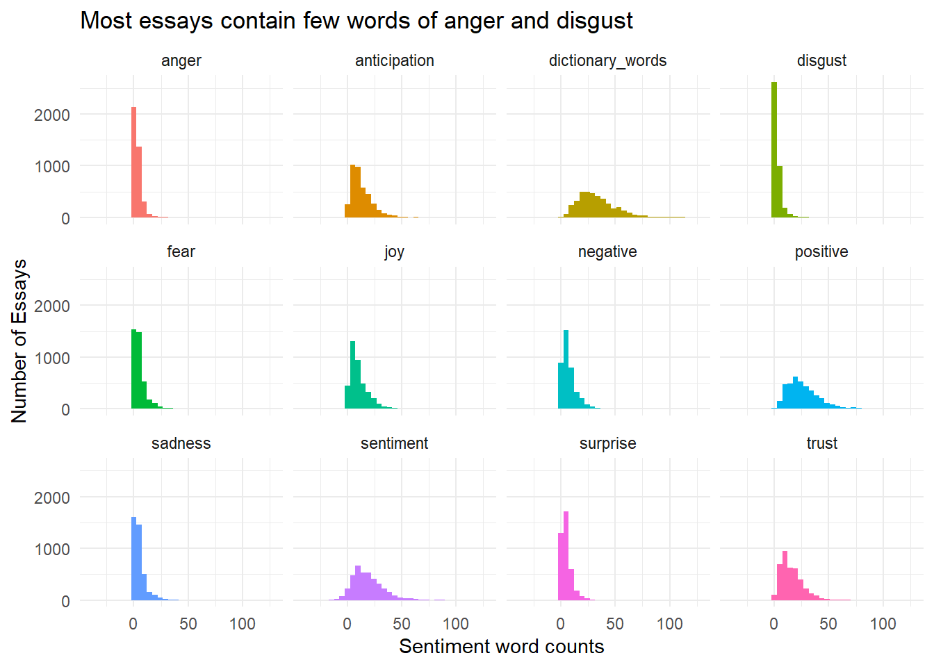

train_essays_sentiment <- train_essays_raw |> 
         bind_cols(sentiment_preprocessor(train_essays_raw))

submit_essays_sentiment <- submit_essays_raw |> 
    bind_cols(sentiment_preprocessor(submit_essays_raw))

Essays with more words, or more sentences, do not necessarily score better.

te_long <- train_essays_raw |>
  pivot_longer(cols = cohesion:conventions,
               names_to = "metric",
               values_to = "value") |>
  mutate(metric = as.factor(metric),
         value = as.factor(value))

te_long |> 
  group_by(n_words = ggplot2::cut_interval(
    tokenizers::count_words(full_text), 
    length = 200),
    metric, value) |> 
  summarise(`Number of essays` = n(),
            .groups = "drop") |> 
  ggplot(aes(n_words, `Number of essays`, fill = as.factor(value))) +
  geom_col() +
  scale_x_discrete(guide = guide_axis(n.dodge = 2)) +
  facet_wrap(vars(metric)) +
  labs(x = "Number of words per essay",
       y = "Number of essays",
       fill = "Score")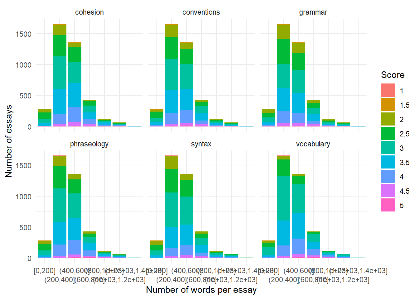

te_long |> 
  group_by(n_words = ggplot2::cut_interval(
    tokenizers::count_sentences(full_text), length = 20),
    metric, value) |> 
  summarise(`Number of essays` = n(),
            .groups = "drop") |> 
  ggplot(aes(n_words, `Number of essays`, fill = as.factor(value))) +
  geom_col() +
  scale_x_discrete(guide = guide_axis(n.dodge = 2)) +
  facet_wrap(vars(metric)) +
  labs(x = "Number of sentences per essay",
       y = "Number of essays",
       fill = "Score")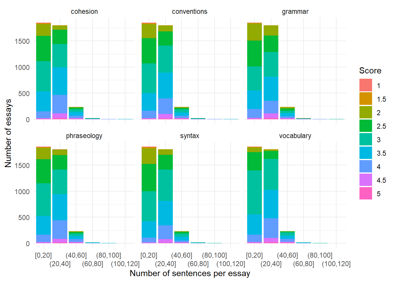

A look at predictor and outcome pairwise correlations.

train_essays_sentiment |> 
 #   select(!!outcomes) %>%
  corrr::correlate(
    quiet = TRUE
  ) %>%
  corrr::rearrange() %>%
  corrr::shave() %>%
  corrr::rplot(print_cor = TRUE) +
  scale_x_discrete(guide = guide_axis(n.dodge = 2))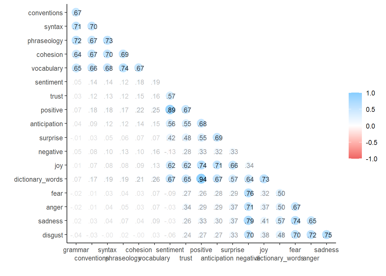

train_essays_sentiment |> 
 #   select(!!outcomes) %>%
  corrr::correlate(
    quiet = TRUE
  ) %>%
  corrr::network_plot()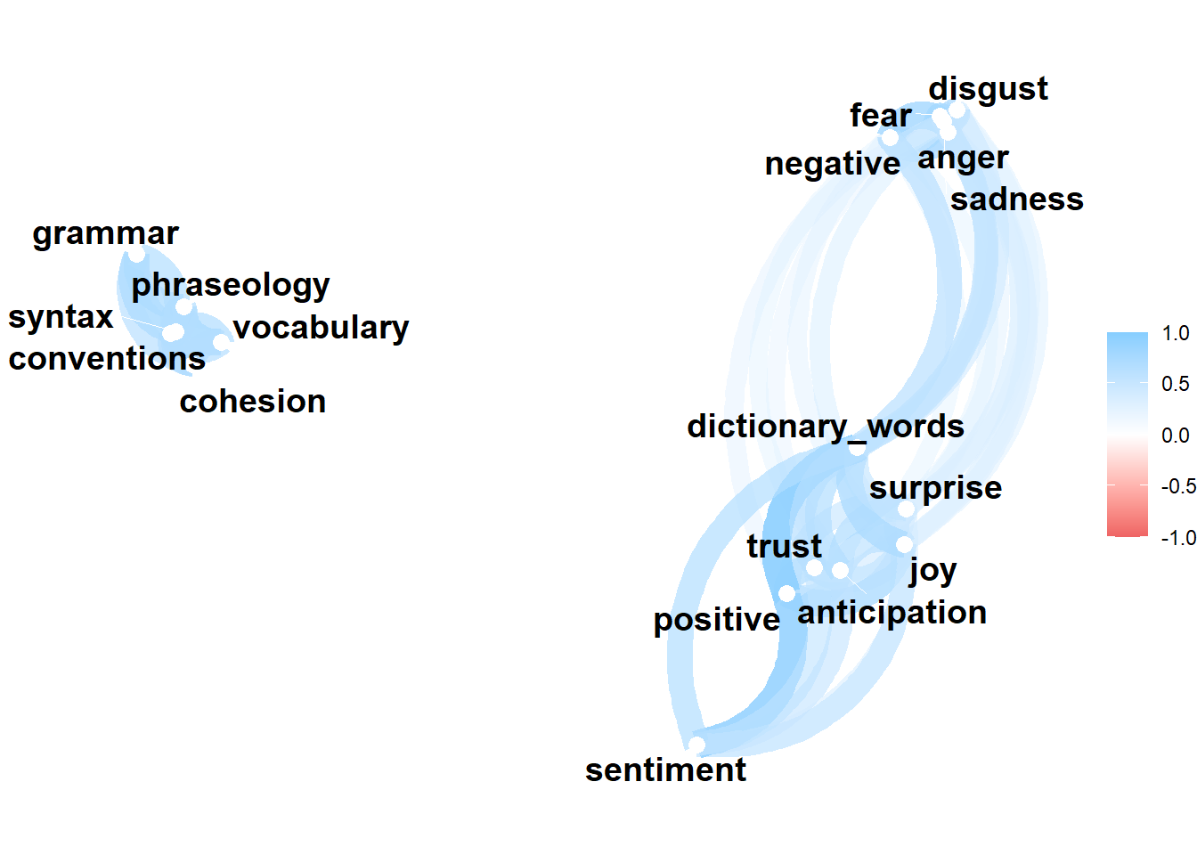

• Vocabulary and Phraseology (0.74) track together.
• Phraseology and Syntax (0.73) track together.
• Praseology and Grammar (0.72) track together.

Let’s set some initial hyperparameters.

# train dataset has 21953 unique one n_gram tokens. 
topics <- 90L   # LDA topic models

Latent Dirichlet allocation (LDA) is an unsupervised generative statistical model that explains a set of observations through unobserved groups, and the content of each group may explain why some parts of the data are similar.

I’d like to explore the use of inverse probability weights because there are so few essays with scores at the highest and lowest levels. When survey respondents have different probabilities of selection, (inverse) probability weights help reduce bias in the results.

I am making us of metaprogramming techniques to pass text vector column names into the formula and case weights functions to re-use them for each metric.

case_weight_builder <- function(data, outcome) {
  data %>%
    inner_join(
      data %>%
        count(.data[[outcome]],
              name = "case_wts"),
      by = glue::glue("{ outcome }")
    ) %>%
    mutate(case_wts = importance_weights(max(case_wts) / case_wts))
}


recipe_builder <- function(outcome = "cohesion",
                           predictor = "full_text",
                           sentiments = "dictionary_words"){

rec <- recipe(formula(glue::glue("{ outcome } ~ { predictor } + { sentiments } + case_wts")),
              data = train_essays_sentiment %>%
                   case_weight_builder(outcome) 
              ) %>%
  step_textfeature(full_text,
                   keep_original_cols = TRUE) %>%
  step_rename_at(
    starts_with("textfeature_"),
    fn = ~ gsub("textfeature_full_text_", "", .)
  ) %>%
  step_mutate(nonwords = n_uq_words - dictionary_words ) %>%
#### cluster the essays by topic, generally
   step_tokenize(full_text) %>% 
   step_lda(full_text, 
            num_topics = topics, 
            keep_original_cols = TRUE) %>%
  step_tfidf(full_text) %>%
  step_clean_names(all_predictors()) %>%
#### remove columns that are super-sparse and unbalanced
  step_nzv(all_predictors(), unique_cut = 9) %>%
  step_normalize(all_numeric_predictors())

return(rec)

}

As mentioned above, the model specification is xgboost for regression to predict a continuous outcome.

# finalize(mtry(), 
#          recipe_builder() |> 
#            prep() |> 
#            bake(new_data = NULL))

spec <-
  boost_tree(
    mtry = 70,  # 75L
    trees = 500L,
    tree_depth = 9, # 6L
    learn_rate = 0.01,  # originally 0.1
    min_n = 20,  # 20L
    loss_reduction = 0
  ) %>%
  set_engine('xgboost') %>%
  set_mode('regression')

# all_cores <- parallelly::availableCores(omit = 1)
# all_cores
# 
# future::plan("multisession", workers = all_cores) # on Windows

We fit for cohesion first and use case weights to adjust for the frequency of occurrence of cohesion. After looking at variable importance (roughly the number of times a variable appears in the trees) and residuals, we make our prediction on the submission set essays and adding that column to the dataframe.

outcome <- outcomes[1]

train_df <- train_essays_sentiment %>%
                   case_weight_builder(outcome)

wf <- workflow(recipe_builder(outcome = outcome, sentiments = sentiments), spec) |> 
       add_case_weights(case_wts)

#
#folds <- vfold_cv(train_df, strata = !!outcome)

#grid <- expand.grid(learn_rate = c(0.006, 0.01, 0.03))

# rs <- tune_grid(
#   wf,
#   folds,
#   grid = grid,
#   metrics = metric_set(rmse),
#   control = control_grid()
# )
#   
# autoplot(rs)
# collect_metrics(rs)

fit <- parsnip::fit(wf, train_df)

as(<dgTMatrix>, "dgCMatrix") is deprecated since Matrix 1.5-0; do as(., "CsparseMatrix") instead

extract_fit_engine(fit) |> 
  vip::vip(num_features = 20)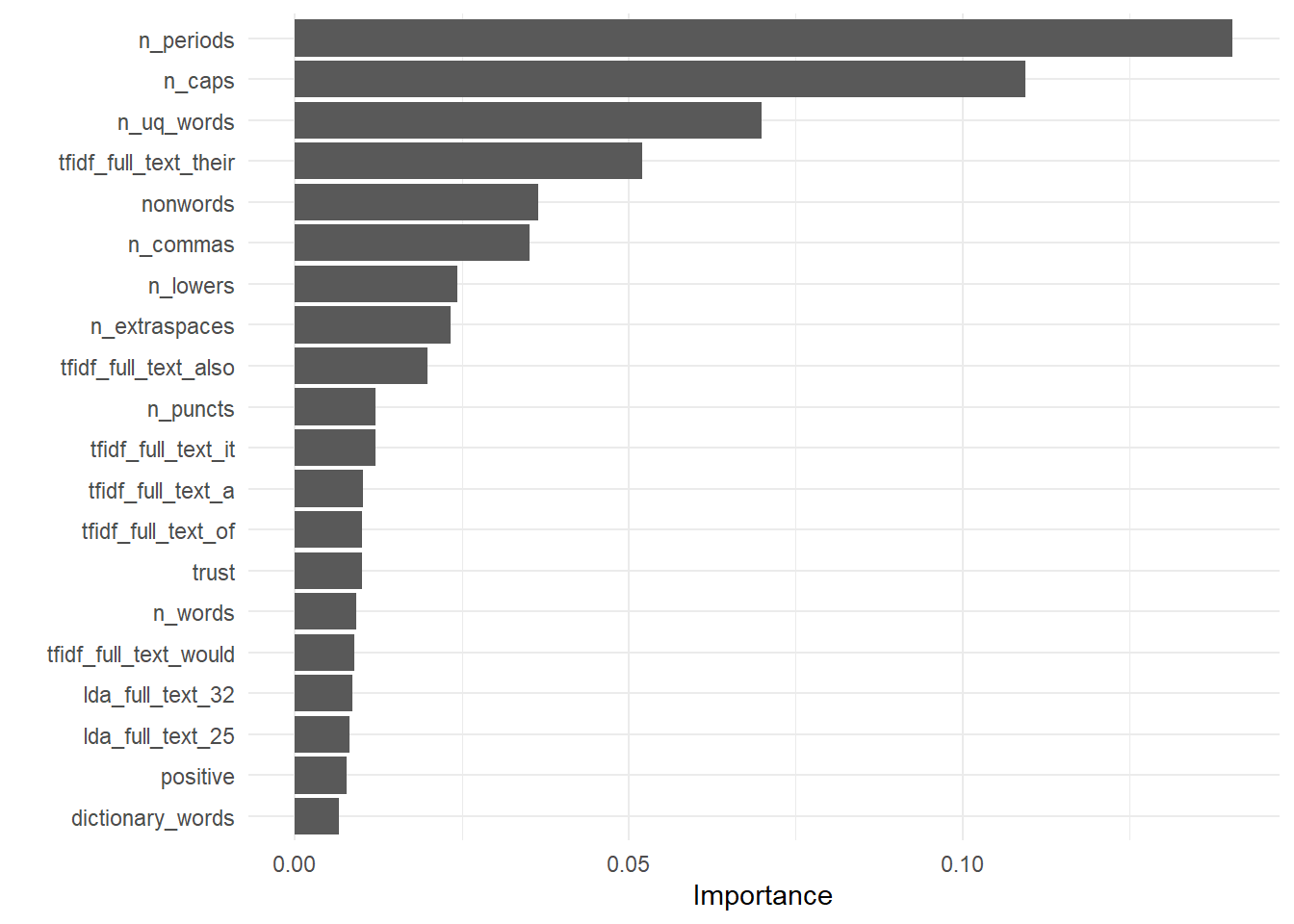

train_preds <- predict(fit, new_data = train_essays_sentiment) |> 
   bind_cols(train_essays_raw |> select(!!outcome)) |> 
   rename(truth = !!outcome)

train_preds |> 
   ggplot(aes(x = factor(truth), y = .pred - truth)) +
   geom_boxplot() +
   labs(title = glue::glue("{ outcome } residuals"))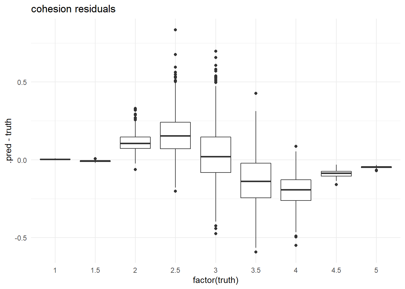 

train_preds %>%
   yardstick::rmse(truth, .pred)

submit_essays_sentiment <- predict(fit, submit_essays_sentiment) |> 
  rename({{outcome}} := .pred) |> 
  bind_cols(submit_essays_sentiment)

Warning in get_dtm(corp): dtm has 0 rows. Empty iterator?

We fit for syntax second and use case weights to adjust for the frequency of occurrence of syntax. I am choosing to use the predicted values of cohesion above as an additional predictor.

outcome <- outcomes[2]
predictor <- glue::glue("full_text + { outcomes[1] }")

train_df <- train_essays_sentiment %>%
                   case_weight_builder(outcome)

wf <- workflow(recipe_builder(outcome, predictor, sentiments), spec) %>%
          add_case_weights(case_wts)

fit <- parsnip::fit(wf, train_df)

extract_fit_engine(fit) |> 
  vip::vip(num_features = 20)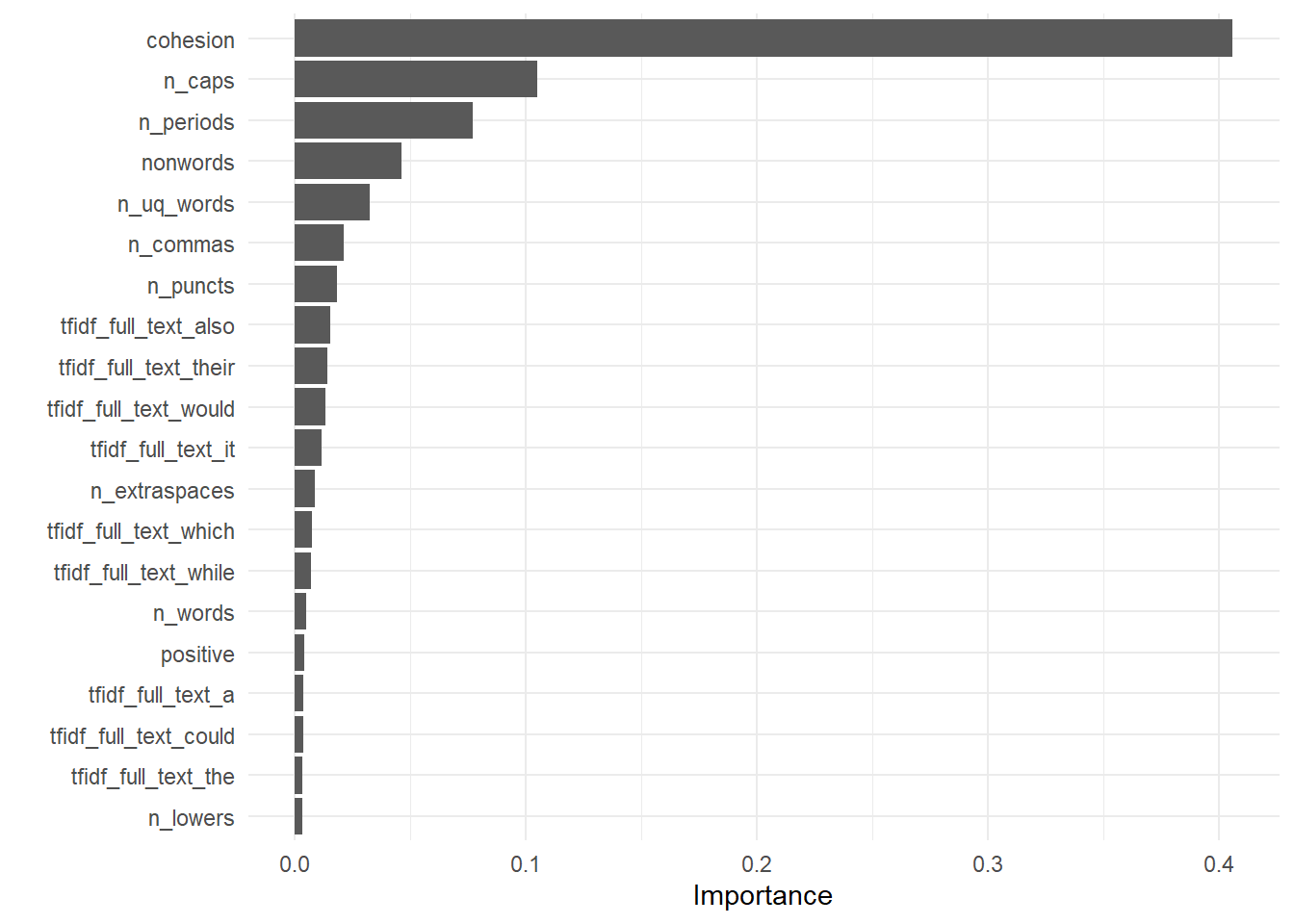

train_preds <- predict(fit, new_data = train_essays_sentiment) |> 
   bind_cols(train_essays_raw |> select(!!outcome)) |> 
   rename(truth = !!outcome)

train_preds |> 
   ggplot(aes(x = factor(truth), y = .pred - truth)) +
   geom_boxplot() +
   labs(title = glue::glue("{ outcome } residuals"))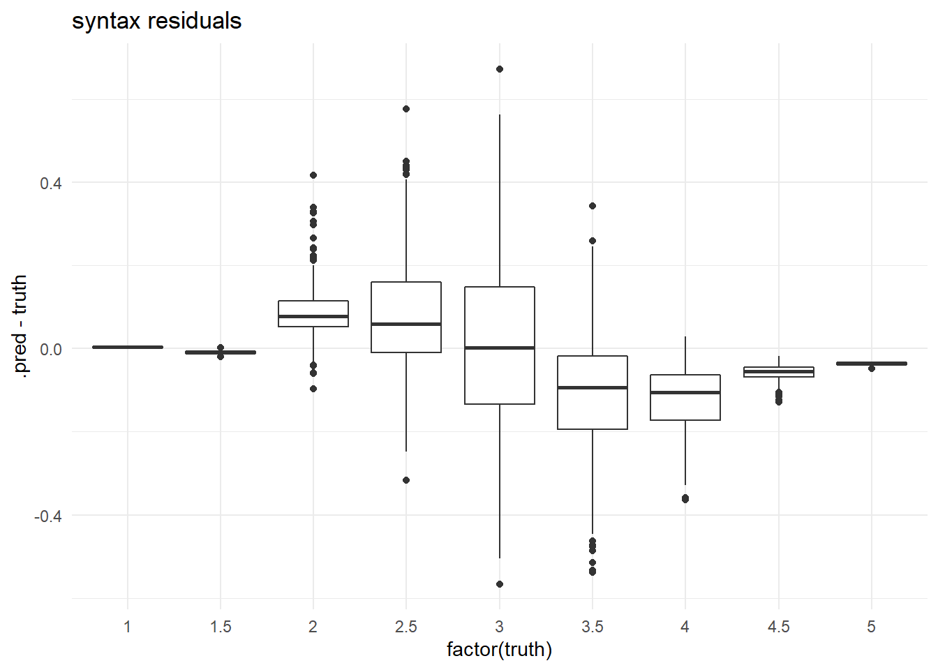 

train_preds %>%
   yardstick::rmse(truth, .pred)

submit_essays_sentiment <- predict(fit, submit_essays_sentiment) |> 
  rename({{outcome}} := .pred) |> 
  bind_cols(submit_essays_sentiment)

Warning in get_dtm(corp): dtm has 0 rows. Empty iterator?

We fit for vocabulary next and use case weights to adjust for the frequency of occurrence of vocabulary. I am choosing to use the predicted values of cohesion and syntax above as additional predictors.

outcome <- outcomes[3]
predictor <- glue::glue("full_text + { outcomes[1] } + { outcomes[2] }")

train_df <- train_essays_sentiment %>%
                   case_weight_builder(outcome)

wf <- workflow(recipe_builder(outcome, predictor, sentiments), spec) %>%
          add_case_weights(case_wts)

fit <- parsnip::fit(wf, train_df)

extract_fit_engine(fit) |> 
  vip::vip(num_features = 20)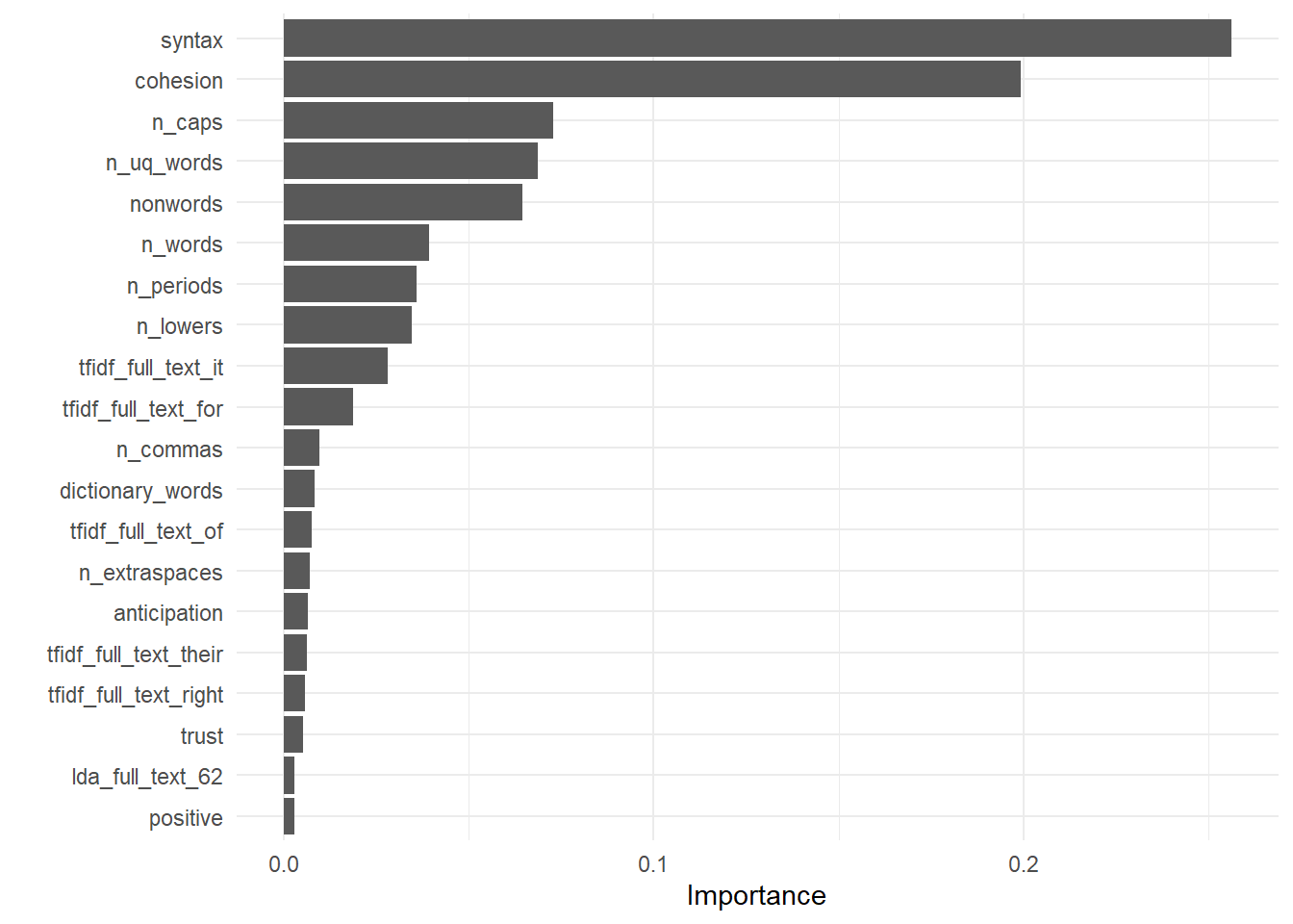

train_preds <- predict(fit, new_data = train_essays_sentiment) |> 
   bind_cols(train_essays_raw |> select(!!outcome)) |> 
   rename(truth = !!outcome)

train_preds |> 
   ggplot(aes(x = factor(truth), y = .pred - truth)) +
   geom_boxplot() +
   labs(title = glue::glue("{ outcome } residuals"))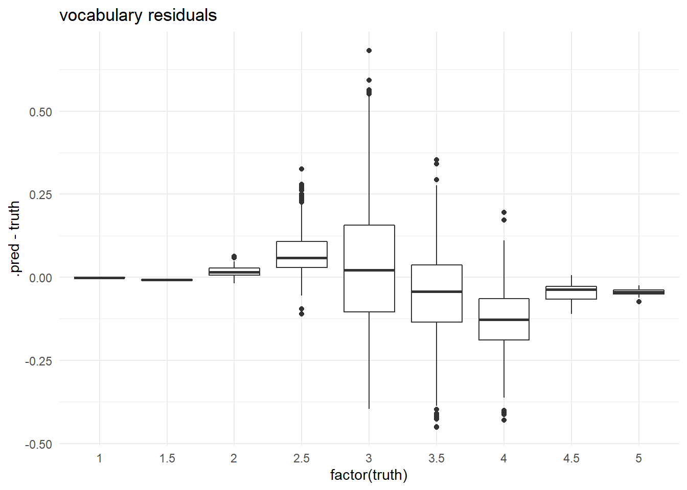 

train_preds %>%
   yardstick::rmse(truth, .pred)

submit_essays_sentiment <- predict(fit, submit_essays_sentiment) |> 
  rename({{outcome}} := .pred) |> 
  bind_cols(submit_essays_sentiment)

Warning in get_dtm(corp): dtm has 0 rows. Empty iterator?

We fit for phraseology next and use case weights to adjust for the frequency of occurrence of phraseology. I am choosing to use the predicted values of cohesion, syntax, and vocabulary above as additional predictors.

outcome <- outcomes[4]
predictor <- glue::glue("full_text + { outcomes[1] } + { outcomes[2] } + { outcomes[3] }")

train_df <- train_essays_sentiment %>%
                   case_weight_builder(outcome)

wf <- workflow(recipe_builder(outcome, predictor, sentiments), spec) %>%
          add_case_weights(case_wts)

fit <- parsnip::fit(wf, train_df)

extract_fit_engine(fit) |> 
  vip::vip(num_features = 20)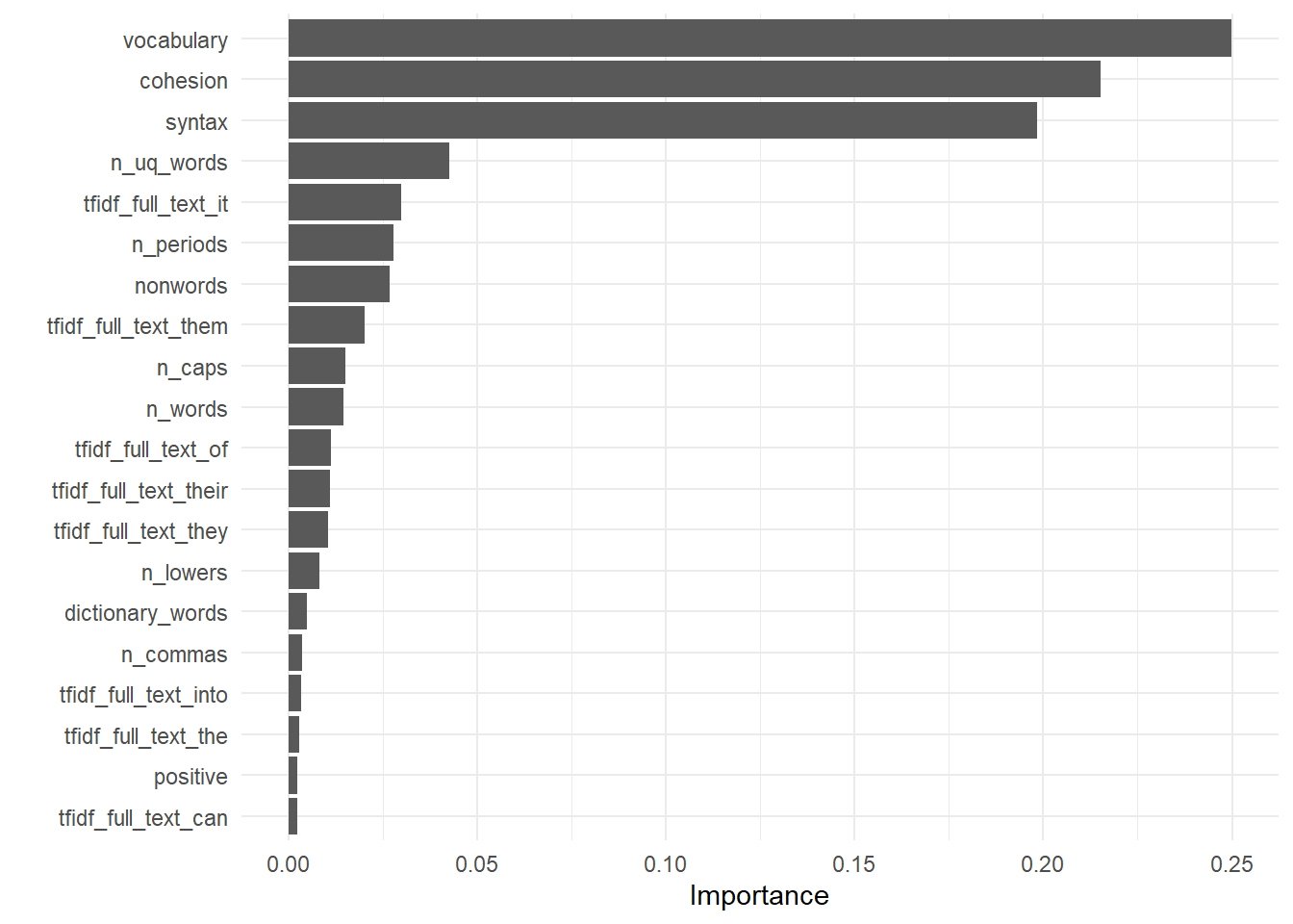

train_preds <- predict(fit, new_data = train_essays_sentiment) |> 
   bind_cols(train_essays_raw |> select(!!outcome)) |> 
   rename(truth = !!outcome)

train_preds |> 
   ggplot(aes(x = factor(truth), y = .pred - truth)) +
   geom_boxplot() +
   labs(title = glue::glue("{ outcome } residuals"))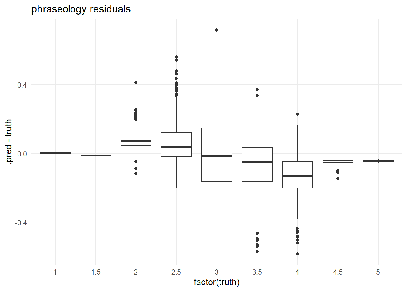 

train_preds %>%
   yardstick::rmse(truth, .pred)

submit_essays_sentiment <- predict(fit, submit_essays_sentiment) |> 
  rename({{outcome}} := .pred) |> 
  bind_cols(submit_essays_sentiment)

Warning in get_dtm(corp): dtm has 0 rows. Empty iterator?

We fit for grammar next and use case weights to adjust for the frequency of occurrence of grammar. I am choosing to use the predicted values of cohesion, syntax, vocabulary, and phraseology above as additional predictors.

outcome <- outcomes[5]
predictor <- glue::glue("full_text + { outcomes[1] } + { outcomes[2]} + {outcomes[3]} + {outcomes[4]}")

train_df <- train_essays_sentiment %>%
                   case_weight_builder(outcome)

wf <- workflow(recipe_builder(outcome, predictor, sentiments), spec) %>%
          add_case_weights(case_wts)

fit <- parsnip::fit(wf, train_df)

extract_fit_engine(fit) |> 
  vip::vip(num_features = 20)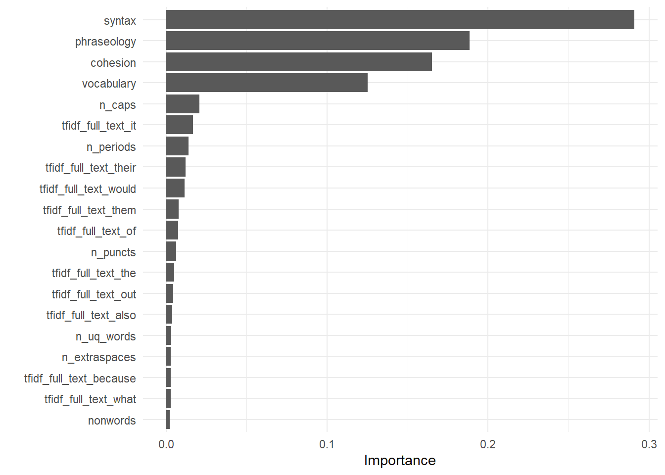

train_preds <- predict(fit, new_data = train_essays_sentiment) |> 
   bind_cols(train_essays_raw |> select(!!outcome)) |> 
   rename(truth = !!outcome)

train_preds |> 
   ggplot(aes(x = factor(truth), y = .pred - truth)) +
   geom_boxplot() +
   labs(title = glue::glue("{ outcome } residuals"))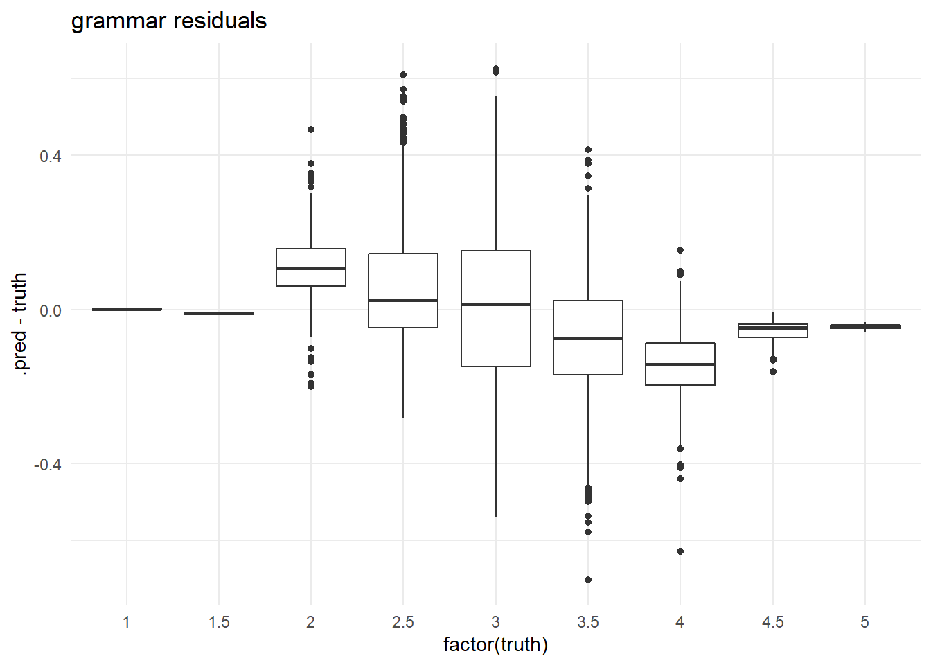 

train_preds %>%
   yardstick::rmse(truth, .pred)

submit_essays_sentiment <- predict(fit, submit_essays_sentiment) |> 
  rename({{outcome}} := .pred) |> 
  bind_cols(submit_essays_sentiment)

Warning in get_dtm(corp): dtm has 0 rows. Empty iterator?

We fit for conventions next and use case weights to adjust for the frequency of occurrence of conventions. I am choosing to use the predicted values of cohesion, syntax, vocabulary, phraseology and grammar above as additional predictors.

outcome <- outcomes[6]
predictor <- glue::glue("full_text + { outcomes[1] } +{ outcomes[2] }+{ outcomes[3] }+{ outcomes[4] }+{ outcomes[5] }")

train_df <- train_essays_sentiment %>%
                   case_weight_builder(outcome)

wf <- workflow(recipe_builder(outcome, predictor, sentiments), spec) %>%
          add_case_weights(case_wts)

fit <- parsnip::fit(wf, train_df)

extract_fit_engine(fit) |> 
  vip::vip(num_features = 20)

train_preds <- predict(fit, new_data = train_essays_sentiment) |> 
   bind_cols(train_essays_raw |> select(!!outcome)) |> 
   rename(truth = !!outcome)

train_preds |> 
   ggplot(aes(x = factor(truth), y = .pred - truth)) +
   geom_boxplot() +
   labs(title = glue::glue("{ outcome } residuals"))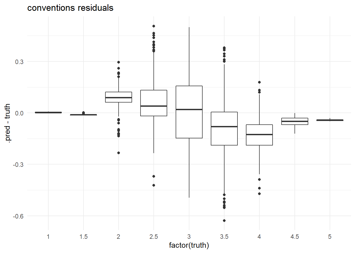 

train_preds %>%
   yardstick::rmse(truth, .pred)

submit_essays_sentiment <- predict(fit, submit_essays_sentiment) |> 
  rename({{outcome}} := .pred) |> 
  bind_cols(submit_essays_sentiment)

Warning in get_dtm(corp): dtm has 0 rows. Empty iterator?

The Submission

submission <-
  submit_essays_sentiment %>%
  select(text_id, !!outcomes)

submission

write_csv(submission, here::here("data", "submission.csv"))

Session information

sessionInfo()

R version 4.2.1 (2022-06-23 ucrt)
Platform: x86_64-w64-mingw32/x64 (64-bit)
Running under: Windows 10 x64 (build 22621)

Matrix products: default

locale:
[1] LC_COLLATE=English_United States.utf8 
[2] LC_CTYPE=English_United States.utf8   
[3] LC_MONETARY=English_United States.utf8
[4] LC_NUMERIC=C                          
[5] LC_TIME=English_United States.utf8    

attached base packages:
[1] stats     graphics  grDevices utils     datasets  methods   base     

other attached packages:
 [1] textrecipes_1.0.1  tidytext_0.3.4     text2vec_0.6.2     stm_1.3.6         
 [5] yardstick_1.1.0    workflowsets_1.0.0 workflows_1.1.0    tune_1.0.1        
 [9] rsample_1.1.0      recipes_1.0.1      parsnip_1.0.2      modeldata_1.0.1   
[13] infer_1.0.3        dials_1.0.0        scales_1.2.1       broom_1.0.1       
[17] tidymodels_1.0.0   forcats_0.5.2      stringr_1.4.1      dplyr_1.0.10      
[21] purrr_0.3.5        readr_2.1.3        tidyr_1.2.1        tibble_3.1.8      
[25] ggplot2_3.3.6      tidyverse_1.3.2    workflowr_1.7.0   

loaded via a namespace (and not attached):
  [1] readxl_1.4.1           backports_1.4.1        splines_4.2.1         
  [4] listenv_0.8.0          SnowballC_0.7.0        digest_0.6.29         
  [7] foreach_1.5.2          htmltools_0.5.3        float_0.3-0           
 [10] fansi_1.0.3            magrittr_2.0.3         memoise_2.0.1         
 [13] googlesheets4_1.0.1    tzdb_0.3.0             globals_0.16.1        
 [16] modelr_0.1.9           gower_1.0.0            vroom_1.6.0           
 [19] hardhat_1.2.0          colorspace_2.0-3       vip_0.3.2             
 [22] ggrepel_0.9.1          rappdirs_0.3.3         rvest_1.0.3           
 [25] haven_2.5.1            xfun_0.33              callr_3.7.2           
 [28] crayon_1.5.2           jsonlite_1.8.2         survival_3.3-1        
 [31] iterators_1.0.14       glue_1.6.2             registry_0.5-1        
 [34] gtable_0.3.1           gargle_1.2.1           ipred_0.9-13          
 [37] future.apply_1.9.1     mlapi_0.1.1            DBI_1.1.3             
 [40] Rcpp_1.0.9             GPfit_1.0-8            bit_4.0.4             
 [43] lava_1.6.10            prodlim_2019.11.13     httr_1.4.4            
 [46] ellipsis_0.3.2         farver_2.1.1           pkgconfig_2.0.3       
 [49] nnet_7.3-17            sass_0.4.2             dbplyr_2.2.1          
 [52] janitor_2.1.0          here_1.0.1             utf8_1.2.2            
 [55] labeling_0.4.2         tidyselect_1.2.0       rlang_1.0.6           
 [58] DiceDesign_1.9         later_1.3.0            munsell_0.5.0         
 [61] cellranger_1.1.0       tools_4.2.1            cachem_1.0.6          
 [64] xgboost_1.6.0.1        cli_3.4.0              corrr_0.4.4           
 [67] generics_0.1.3         rsparse_0.5.1          evaluate_0.17         
 [70] fastmap_1.1.0          yaml_2.3.5             textdata_0.4.4        
 [73] processx_3.7.0         RhpcBLASctl_0.21-247.1 knitr_1.40            
 [76] bit64_4.0.5            fs_1.5.2               lgr_0.4.4             
 [79] future_1.28.0          whisker_0.4            textfeatures_0.3.3    
 [82] xml2_1.3.3             tokenizers_0.2.3       compiler_4.2.1        
 [85] rstudioapi_0.14        reprex_2.0.2           lhs_1.1.5             
 [88] bslib_0.4.0            stringi_1.7.8          highr_0.9             
 [91] ps_1.7.1               lattice_0.20-45        Matrix_1.5-1          
 [94] conflicted_1.1.0       vctrs_0.4.2            pillar_1.8.1          
 [97] lifecycle_1.0.3        furrr_0.3.1            jquerylib_0.1.4       
[100] data.table_1.14.2      seriation_1.3.6        httpuv_1.6.6          
[103] R6_2.5.1               TSP_1.2-1              promises_1.2.0.1      
[106] gridExtra_2.3          janeaustenr_1.0.0      parallelly_1.32.1     
[109] codetools_0.2-18       MASS_7.3-57            assertthat_0.2.1      
[112] rprojroot_2.0.3        withr_2.5.0            parallel_4.2.1        
[115] hms_1.1.2              grid_4.2.1             rpart_4.1.16          
[118] timeDate_4021.106      class_7.3-20           snakecase_0.11.0      
[121] rmarkdown_2.17         googledrive_2.0.0      git2r_0.30.1          
[124] getPass_0.2-2          lubridate_1.8.0