Hai Duong: Measles

workflowr

• Summary
• Checks
• Past versions

Last updated: 2022-08-25

Checks: 6 1

Knit directory: Vaccination_COVID/

This reproducible R Markdown analysis was created with workflowr (version 1.7.0). The Checks tab describes the reproducibility checks that were applied when the results were created. The Past versions tab lists the development history.

---

R Markdown file: uncommitted changes

The R Markdown file has unstaged changes. To know which version of the R Markdown file created these results, you’ll want to first commit it to the Git repo. If you’re still working on the analysis, you can ignore this warning. When you’re finished, you can run wflow_publish to commit the R Markdown file and build the HTML.

Environment: empty

Great job! The global environment was empty. Objects defined in the global environment can affect the analysis in your R Markdown file in unknown ways. For reproduciblity it’s best to always run the code in an empty environment.

Seed: set.seed(20210126)

The command set.seed(20210126) was run prior to running the code in the R Markdown file. Setting a seed ensures that any results that rely on randomness, e.g. subsampling or permutations, are reproducible.

Session information: recorded

Great job! Recording the operating system, R version, and package versions is critical for reproducibility.

Cache: none

Nice! There were no cached chunks for this analysis, so you can be confident that you successfully produced the results during this run.

File paths: relative

Great job! Using relative paths to the files within your workflowr project makes it easier to run your code on other machines.

Repository version: 8629620

Great! You are using Git for version control. Tracking code development and connecting the code version to the results is critical for reproducibility.

The results in this page were generated with repository version 8629620. See the Past versions tab to see a history of the changes made to the R Markdown and HTML files.

Note that you need to be careful to ensure that all relevant files for the analysis have been committed to Git prior to generating the results (you can use wflow_publish or wflow_git_commit). workflowr only checks the R Markdown file, but you know if there are other scripts or data files that it depends on. Below is the status of the Git repository when the results were generated:

Ignored files:
    Ignored:    .DS_Store
    Ignored:    .Rhistory
    Ignored:    .Rproj.user/
    Ignored:    analysis/.DS_Store
    Ignored:    analysis/.Rhistory
    Ignored:    code/.DS_Store

Unstaged changes:
    Modified:   analysis/haiduong_measles.Rmd

Note that any generated files, e.g. HTML, png, CSS, etc., are not included in this status report because it is ok for generated content to have uncommitted changes.

---

These are the previous versions of the repository in which changes were made to the R Markdown (analysis/haiduong_measles.Rmd) and HTML (docs/haiduong_measles.html) files. If you’ve configured a remote Git repository (see ?wflow_git_remote), click on the hyperlinks in the table below to view the files as they were in that past version.

File	Version	Author	Date	Message
Rmd	8629620	thinhong	2022-08-25	add vaccine coverage and confidence interval
html	8629620	thinhong	2022-08-25	add vaccine coverage and confidence interval

---

knitr::opts_chunk$set(echo = T, warning = F, message = F, out.width = "100%")

library(data.table)
library(dplyr)

Warning: package 'dplyr' was built under R version 4.1.2

Attaching package: 'dplyr'

The following objects are masked from 'package:data.table':

    between, first, last

The following objects are masked from 'package:stats':

    filter, lag

The following objects are masked from 'package:base':

    intersect, setdiff, setequal, union

library(tidyr)

Warning: package 'tidyr' was built under R version 4.1.2

library(lubridate)

Attaching package: 'lubridate'

The following objects are masked from 'package:data.table':

    hour, isoweek, mday, minute, month, quarter, second, wday, week,
    yday, year

The following objects are masked from 'package:base':

    date, intersect, setdiff, union

library(ggplot2)
library(gtsummary)

Warning: package 'gtsummary' was built under R version 4.1.2

library(ggsci)
library(plotly)

Attaching package: 'plotly'

The following object is masked from 'package:ggplot2':

    last_plot

The following object is masked from 'package:stats':

    filter

The following object is masked from 'package:graphics':

    layout

datap <- file.path("~", "Downloads", "updated_dataset")

covidvc <- readRDS(file.path(datap, "Combined_VAC_COVID19_2022-02-17.rds"))
measle_all <- readRDS(file.path(datap, "measles_haiduong.rds"))
measle_all <- data.table(measle_all)

hepb <- readRDS(file.path(datap, "hepb_haiduong.rds"))
hepb <- data.table(hepb)
hepb <- hepb[which(hepb$shot == 1),]

time_step <- "month"
measle_all$vacym <- floor_date(measle_all$vacdate, time_step)
measle_all$vacname2 <- factor(measle_all$vacname2, levels = c("Measles", "MR", "MMR"))

# measle_all <- measle_all %>%
#   group_by(pid) %>%
#   arrange(vacdate) %>%
#   mutate(shot_any = 1:n()) %>%
#   ungroup()
# 
# table(measle_all$shot_any)
# table(measle_all$shot)

Measles and COVID-19 vaccination per month

covidvc <- covidvc[which(covidvc$location == "Hai Duong"),]
covidvc$total_shots <- rowSums(covidvc[,c("vaccinated_1st", "vaccinated_2nd", "vaccinated_3rd")], na.rm = T)

covidvc$vacym <- floor_date(covidvc$date, time_step)
covidvc$vacyear <- year(covidvc$vacym)
covidvc$vacmonth <- month(covidvc$vacym)

covid <- covidvc %>% 
  group_by(vacyear, vacmonth) %>%
  summarise(n = sum(total_shots))

covid$vacname2 <- "COVID vaccine"
covid$n <- covid$n / 50

df_plot <- measle_all %>% 
    count(vacyear, vacmonth, vacname2)

df_plot <- rbind(df_plot, covid)

ggplot(df_plot, aes(x = vacmonth, y = n, color = vacname2)) +
  geom_line(stat = "identity") +
  facet_wrap(~ vacyear) +
  scale_x_continuous(breaks = scales::pretty_breaks(n = 6)) +
  labs(x = NULL) +
  theme_light()

Past versions of unnamed-chunk-3-1.png

Version	Author	Date
8629620	thinhong	2022-08-25

• High peak of MR shots in Nov 2019
• No disruption in Apr 2020
• Disruptions in Aug 2020 and Feb 2021

Vaccination campaign in Nov 2019

An MR vaccination campaign is triggered during this time in Hai Duong, focusing on children 1-5 year-old

tmp_year <- 2019
tmp <- measle_all[which(measle_all$vacyear == tmp_year),]

ggplot(tmp, aes(x = vagem)) +
  geom_histogram() +
  facet_wrap(~ vacmonth, scales = "free") +
  scale_x_continuous(breaks = scales::pretty_breaks(n = 5)) +
  labs(x = "Age at vaccination (months)") +
  ggtitle(tmp_year)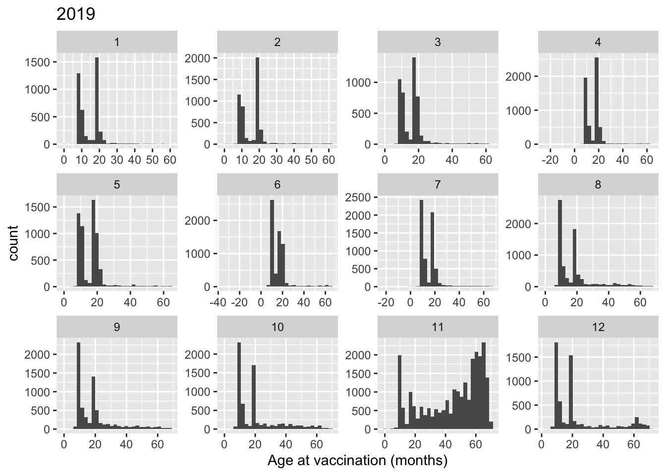

Past versions of unnamed-chunk-4-1.png

Version	Author	Date
8629620	thinhong	2022-08-25

No disruption in Apr 2020 but in Aug 2020 and Feb 2021

The monthly vaccination date at public clinics is usually at the end of the month. In Mar 2020: right before lockdown they vaccinate children and right after lockdown they came back to vaccinate children

Hai Duong had a Hai Duong city-wide lockdown from 14/8-28/8, this time looks like they only organised the vaccination day in Sep so all children scheduled in Aug miss the shot

tmp_vacyear <- 2020
tmp <- measle_all[which(measle_all$vacyear == tmp_vacyear),]

df_plot <- tmp %>% 
    count(vacdate, vacname2)

ggplot(df_plot, aes(x = vacdate, y = n, color = vacname2)) +
  geom_rect(aes(xmin = ymd("2020-04-01"), xmax = ymd("2020-04-21"), ymin = -Inf, ymax = Inf), fill = "grey90", color = NA, alpha = 0.3) +
  geom_rect(aes(xmin = ymd("2020-08-14"), xmax = ymd("2020-08-28"), ymin = -Inf, ymax = Inf), fill = "grey90", color = NA, alpha = 0.3) +
  geom_line(stat = "identity") +
  scale_x_date(date_breaks = "1 month", labels = scales::date_format("%b")) +
  labs(x = NULL) +
  theme_light() +
  ggtitle(tmp_vacyear)

Past versions of unnamed-chunk-5-1.png

Version	Author	Date
8629620	thinhong	2022-08-25

Zoom in 2021

Hai Duong had a province-wide lockdown from 28/1/2021 - 15/2 (Directive 15), 16/2 - 2/3 (Directive 16), 3/3 - 17/3 (Directive 15), 18/3 - 31/3 (Directive 19)

Directive 16 > 15 > 19

tmp_vacyear <- 2021
tmp <- measle_all[which(measle_all$vacyear == tmp_vacyear),]

df_plot <- tmp %>% 
    count(vacdate, vacname2)

ggplot(df_plot, aes(x = vacdate, y = n, color = vacname2)) +
  geom_rect(aes(xmin = ymd("2021-01-28"), xmax = ymd("2021-02-15"), ymin = -Inf, ymax = Inf), fill = "grey90", color = NA, alpha = 0.5) +
  geom_rect(aes(xmin = ymd("2021-02-16"), xmax = ymd("2021-03-02"), ymin = -Inf, ymax = Inf), fill = "grey90", color = NA, alpha = 0.5) +
  geom_rect(aes(xmin = ymd("2021-03-03"), xmax = ymd("2021-03-17"), ymin = -Inf, ymax = Inf), fill = "grey90", color = NA, alpha = 0.5) +
  geom_rect(aes(xmin = ymd("2021-03-18"), xmax = ymd("2021-03-31"), ymin = -Inf, ymax = Inf), fill = "wheat", color = NA, alpha = 0.5) +
  geom_line(stat = "identity") +
  scale_x_date(date_breaks = "1 month", labels = scales::date_format("%b")) +
  labs(x = NULL) +
  theme_light() +
  ggtitle(tmp_vacyear)

Past versions of unnamed-chunk-6-1.png

Version	Author	Date
8629620	thinhong	2022-08-25

Public vs private

First let decide how a shot is public or private

table(measle_all$clinic_type)

hospital    other  private   public  unknown 
     389     2171    36149   353342    12616 

measle_all$type2 <- ifelse(
  measle_all$clinic_type %in% c("unknown", "other"),
  measle_all$vactype, 
  ifelse(
    measle_all$clinic_type == "hospital",
    "private", 
    measle_all$clinic_type
  )
)
measle_all$type2 <- ifelse(measle_all$type2 == "campaign", "public", measle_all$type2)
# table(measle_all$type2)

Extract children who get 2 shots

measles_2shots <- measle_all[duplicated(measle_all$pid) | duplicated(measle_all$pid, fromLast = T),]

dup_sameday <- measles_2shots[duplicated(measles_2shots[,c("pid", "vacdate")]) |
                                duplicated(measles_2shots[,c("pid", "vacdate")], fromLast = T),
                              c("pid", "vacdate", "vacname2", "type2")]
dup_sameday <- dup_sameday[order(dup_sameday$pid),]
# head(dup_sameday, 10)

Some received the same vaccine in the same day, filter them out and continue

# Remove children with multiple shots of measles in the same day
measles_2shots <- measles_2shots %>%
  distinct(., pid, vacdate, .keep_all = T)

# Now subset the one still get 2 shots
measles_2shots <- measles_2shots[duplicated(measles_2shots$pid) | duplicated(measles_2shots$pid, fromLast = T),]

# Sort by vaccination date and numbering the shot
measles_2shots <- measles_2shots %>%
  group_by(pid) %>%
  arrange(vacdate) %>%
  mutate(vtimes = 1:n(),
         vacdate_1st = first(vacdate)) %>%
  ungroup()

# How many shots they receive
# table(measles_2shots$vtimes)

Some received 3 shots, filtered them out.

# Remove those who get the 3rd shot
measles_2shots <- measles_2shots[measles_2shots$vtimes != 3,]
measles_2shots <- measles_2shots[order(measles_2shots$pid),]

# Prefix "shot" to vtimes to make wide data frame easier
measles_2shots$vtimes <- paste0("shot", measles_2shots$vtimes)

Change dataset from long to wide format

df <- measles_2shots[, c("pid", "vacdate_1st", "vtimes", "type2")]
df <- df %>%
  pivot_wider(., names_from = vtimes, values_from = type2)

df$vyear_1st <- year(df$vacdate_1st)
df$vmonth_1st <- month(df$vacdate_1st)

# head(df)

Aggregate them by month

df_type <- aggregate(pid ~ vyear_1st + vmonth_1st + shot1 + shot2, data = df, FUN = length)

df_type <- df_type %>%
  group_by(vyear_1st, vmonth_1st, shot1) %>%
  mutate(denom = sum(pid))

df_type$pct2 <- 100 * df_type$pid / df_type$denom

res <- t(apply(df_type[,c("pid", "denom")], 1, FUN = function(x) {
  rr <- binom.test(x[1], x[2])
  with(rr, c(x, 
             "low_ci" = 100 * conf.int[1],
             "high_ci" = 100 * conf.int[2]))
}))

res <- cbind(res, df_type[,grep("pid|denom", colnames(df_type), invert = T)])

# Take 01/2018 as an example
# df_type %>%
#   filter(vyear_1st == 2018 & vmonth_1st == 1) %>%
#   print()

Line plot

# Get only row that 2nd shot is private
df_plot <- res[res$shot2 == "private",]

# To plot on a date format x-axis
df_plot$vacdate_1st <- ym(paste0(df_plot$vyear_1st, "-", df_plot$vmonth_1st))

# Subset from 09/2017 to 03/2020
df_plot <- df_plot[df_plot$vacdate_1st >= "2018-01-01" &
                     df_plot$vacdate_1st <= "2021-11-01",]

df_plot$shot1 <- factor(df_plot$shot1, levels = c("public", "private"))

ggplot(df_plot, aes(x = vacdate_1st, y = pct2, group = shot1)) +
  geom_line(aes(linetype = shot1), stat = "identity", size = 1.1) +
  geom_ribbon(aes(ymin = low_ci, ymax = high_ci, fill = shot1), alpha = 0.25) +
  # geom_vline(xintercept=as.numeric(as.Date("2019-07-01")), color = "orange") +
  scale_x_date(date_labels = "%b-%Y", date_breaks = "1 month") +
  ylim(c(0, 100)) +
  theme_minimal() +
  labs(x = "Month of receiving 1st dose", y = "% 2nd dose in private", linetype = "1st dose in") +
  theme(axis.text.x = element_text(angle = -45, hjust = -0.1),
        panel.grid.minor.x = element_blank())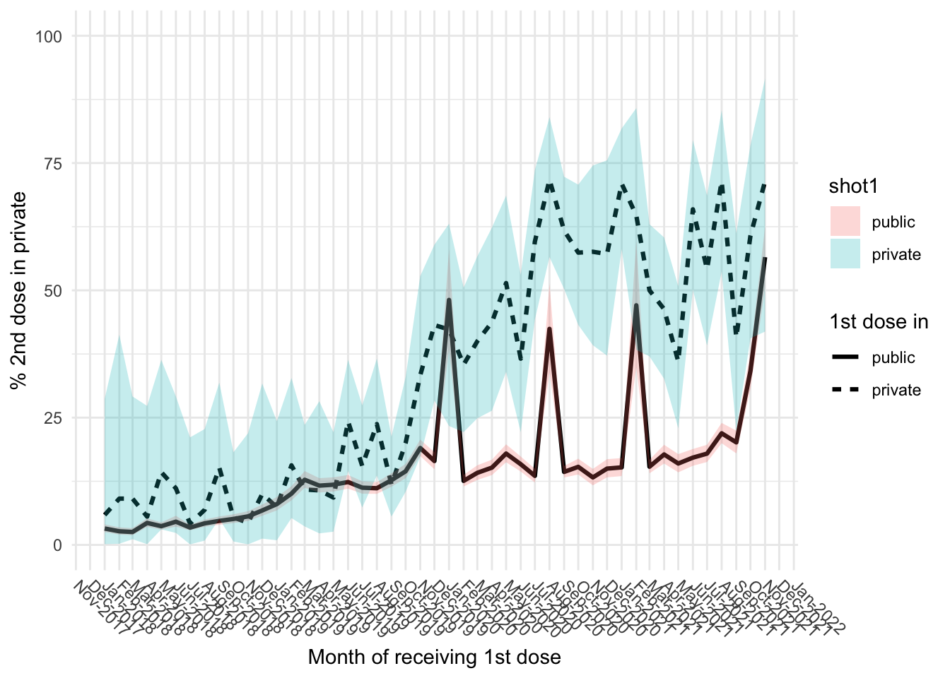

Past versions of unnamed-chunk-13-1.png

Version	Author	Date
8629620	thinhong	2022-08-25

tmp <- df_plot[df_plot$vacdate_1st %in% as.Date(c("2020-01-01", "2020-08-01", "2021-02-01")),]
tmp[order(tmp$vacdate_1st),]

# A tibble: 6 × 10
    pid denom low_ci high_ci vyear_1st vmonth_1st shot1   shot2  pct2 vacdate_…¹
  <dbl> <dbl>  <dbl>   <dbl>     <dbl>      <dbl> <fct>   <chr> <dbl> <date>    
1    11    26   23.4    63.1      2020          1 private priv…  42.3 2020-01-01
2    51   106   38.3    58.0      2020          1 public  priv…  48.1 2020-01-01
3    33    46   56.5    84.0      2020          8 private priv…  71.7 2020-08-01
4    56   132   33.9    51.3      2020          8 public  priv…  42.4 2020-08-01
5    11    17   38.3    85.8      2021          2 private priv…  64.7 2021-02-01
6    32    68   34.8    59.6      2021          2 public  priv…  47.1 2021-02-01
# … with abbreviated variable name ¹​vacdate_1st

tmp <- df_plot[df_plot$vacdate_1st >= "2021-03-01",]
tmp[order(tmp$vacdate_1st),]

# A tibble: 18 × 10
     pid denom low_ci high_ci vyear_1st vmonth_1st shot1  shot2  pct2 vacdate_…¹
   <dbl> <dbl>  <dbl>   <dbl>     <dbl>      <dbl> <fct>  <chr> <dbl> <date>    
 1    31    62   37.0    63.0      2021          3 priva… priv…  50   2021-03-01
 2   445  2897   14.1    16.7      2021          3 public priv…  15.4 2021-03-01
 3    25    54   32.6    60.4      2021          4 priva… priv…  46.3 2021-04-01
 4   304  1711   16.0    19.7      2021          4 public priv…  17.8 2021-04-01
 5    18    50   22.9    50.8      2021          5 priva… priv…  36   2021-05-01
 6   266  1664   14.3    17.8      2021          5 public priv…  16.0 2021-05-01
 7    29    44   50.1    79.5      2021          6 priva… priv…  65.9 2021-06-01
 8   354  2065   15.5    18.8      2021          6 public priv…  17.1 2021-06-01
 9    26    48   39.2    68.6      2021          7 priva… priv…  54.2 2021-07-01
10   364  2030   16.3    19.7      2021          7 public priv…  17.9 2021-07-01
11    25    35   53.7    85.4      2021          8 priva… priv…  71.4 2021-08-01
12   372  1697   20.0    24.0      2021          8 public priv…  21.9 2021-08-01
13    11    27   22.4    61.2      2021          9 priva… priv…  40.7 2021-09-01
14   258  1281   18.0    22.4      2021          9 public priv…  20.1 2021-09-01
15    17    28   40.6    78.5      2021         10 priva… priv…  60.7 2021-10-01
16   237   694   30.6    37.8      2021         10 public priv…  34.1 2021-10-01
17    10    14   41.9    91.6      2021         11 priva… priv…  71.4 2021-11-01
18   156   276   50.4    62.5      2021         11 public priv…  56.5 2021-11-01
# … with abbreviated variable name ¹​vacdate_1st

Population level

df <- measle_all[, c("pid", "province", "vacyear", "vacmonth", "type2")]
df_type <- aggregate(pid ~ vacyear + vacmonth + type2, data = df, FUN = length)

# Percentage of private
df_type <- df_type %>%
  group_by(vacyear, vacmonth) %>%
  mutate(denom = sum(pid))

df_type$pct <- 100 * df_type$pid / df_type$denom



# Get only row that 2nd shot is private
df_plot <- df_type[df_type$type2 == "private",]

# To plot on a date format x-axis
df_plot$vacdate <- ym(paste0(df_plot$vacyear, "-", df_plot$vacmonth))
df_plot <- df_plot[df_plot$vacdate >= "2017-09-01",]

ggplot(df_plot, aes(x = vacdate, y = pct)) +
  geom_line(stat = "identity") +
  # geom_vline(xintercept=as.numeric(as.Date("2020-04-01")), color = "orange") +
  labs(y = "Percentage of private shot (%)", x = "Month of receiving shot") +
  theme_minimal()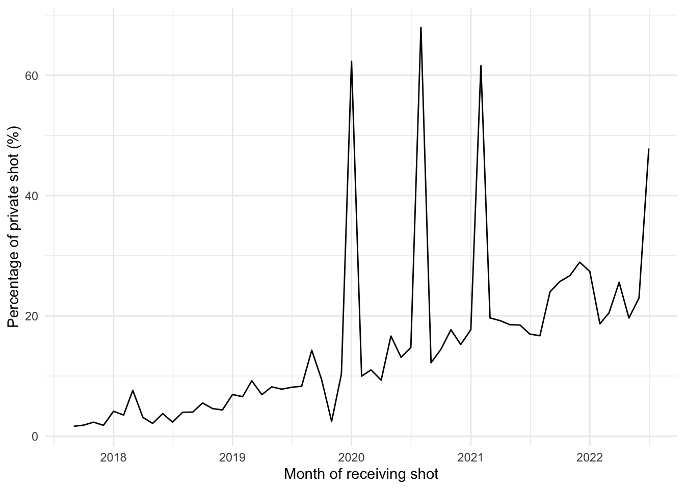

Past versions of unnamed-chunk-16-1.png

Version	Author	Date
8629620	thinhong	2022-08-25

Children who got 2 shots

ggplot(measles_2shots, aes(x = vdelay)) +
  geom_histogram() +
  facet_wrap(~ vacname2, scales = "free")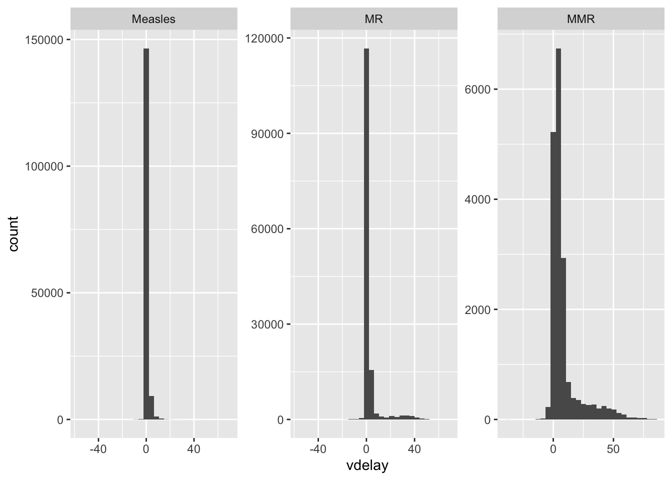

Past versions of unnamed-chunk-17-1.png

Version	Author	Date
8629620	thinhong	2022-08-25

tmp <- measle_all[which(measle_all$vacname2 == "MMR"),]
table(tmp$shot)

    1 
49723 

hepb$dob_ym <- floor_date(hepb$dob, time_step)
measle_all$dob_ym <- floor_date(measle_all$dob, time_step)
measle_all$vac_ym <- floor_date(measle_all$vacdate, time_step)

Children born in 2019 received Measles

yr <- 2019

# Make a vector contains 12 months in the year of interest
start_yr <- ym(paste0(yr, "-01"))
end_yr <- ym(paste0(yr, "-12"))
range_yr <- seq(start_yr, end_yr, "months")

d <- list()

for (i in 1:length(range_yr)) {
  
  l <- list()
  
  # Get the month of birth of this cohort
  cohort <- range_yr[i]
  
  # Number of kids taken from Hep B
  kids <- hepb %>% 
    filter(
      dob_ym == cohort
    ) %>% 
    nrow()
  
  for (j in 1:12) {
    
    # Measles vaccine: 9 month after month of birth
    start_shots <- cohort + months(9)
    
    # The range to get cumulative vaccine coverage
    end_shots <- start_shots + months(j - 1)
  
    shots <- measle_all %>% 
      filter(
        dob_ym == cohort,
        # Month of vaccination between start and end
        vac_ym >= start_shots,
        vac_ym <= end_shots,
        vacname2 %in% c("Measles")
      ) %>%
      distinct(., pid, .keep_all = T) %>%
      nrow()
    
    l[[j]] <- data.frame(
      cohort = cohort, 
      month_cov = end_shots,
      n_month = j + 8, 
      cov = shots / kids
      )
  }
  
  d[[i]] <- do.call(rbind, l)
}

df_plot <- do.call(rbind, d)
df_plot$cohort <- factor(df_plot$cohort)

plot_ly(df_plot, x = ~n_month, y = ~cov, color = ~cohort,
        type = "scatter", mode = "lines",
        hovertext = paste0("Cohort: ", df_plot$cohort, "<br>",
                           "Cutoff month: ", df_plot$month_cov, "<br>",
                           "Coverage: ", df_plot$cov),
        hoverinfo = "text")

Children born in 2019 received Measles or MR

yr <- 2019

# Make a vector contains 12 months in the year of interest
start_yr <- ym(paste0(yr, "-01"))
end_yr <- ym(paste0(yr, "-12"))
range_yr <- seq(start_yr, end_yr, "months")

d <- list()

for (i in 1:length(range_yr)) {
  
  l <- list()
  
  # Get the month of birth of this cohort
  cohort <- range_yr[i]
  
  # Number of kids taken from Hep B
  kids <- hepb %>% 
    filter(
      dob_ym == cohort
    ) %>% 
    nrow()
  
  for (j in 1:12) {
    
    # Measles vaccine: 9 month after month of birth
    start_shots <- cohort + months(9)
    
    # The range to get cumulative vaccine coverage
    end_shots <- start_shots + months(j - 1)
  
    shots <- measle_all %>% 
      filter(
        dob_ym == cohort,
        # Month of vaccination between start and end
        vac_ym >= start_shots,
        vac_ym <= end_shots,
        vacname2 %in% c("Measles", "MR")
      ) %>%
      distinct(., pid, .keep_all = T) %>%
      nrow()
    
    l[[j]] <- data.frame(
      cohort = cohort, 
      month_cov = end_shots,
      n_month = j + 8, 
      cov = shots / kids
      )
  }
  
  d[[i]] <- do.call(rbind, l)
}

df_plot <- do.call(rbind, d)
df_plot$cohort <- factor(df_plot$cohort)

plot_ly(df_plot, x = ~n_month, y = ~cov, color = ~cohort,
        type = "scatter", mode = "lines",
        hovertext = paste0("Cohort: ", df_plot$cohort, "<br>",
                           "Cutoff month: ", df_plot$month_cov, "<br>",
                           "Coverage: ", df_plot$cov),
        hoverinfo = "text")

Children born in 2019 received Measles or MR or MMR

yr <- 2019

# Make a vector contains 12 months in the year of interest
start_yr <- ym(paste0(yr, "-01"))
end_yr <- ym(paste0(yr, "-12"))
range_yr <- seq(start_yr, end_yr, "months")

d <- list()

for (i in 1:length(range_yr)) {
  
  l <- list()
  
  # Get the month of birth of this cohort
  cohort <- range_yr[i]
  
  # Number of kids taken from Hep B
  kids <- hepb %>% 
    filter(
      dob_ym == cohort
    ) %>% 
    nrow()
  
  for (j in 1:12) {
    
    # Measles vaccine: 9 month after month of birth
    start_shots <- cohort + months(9)
    
    # The range to get cumulative vaccine coverage
    end_shots <- start_shots + months(j - 1)
  
    shots <- measle_all %>% 
      filter(
        dob_ym == cohort,
        # Month of vaccination between start and end
        vac_ym >= start_shots,
        vac_ym <= end_shots,
        vacname2 %in% c("Measles", "MR", "MMR")
      ) %>%
      distinct(., pid, .keep_all = T) %>%
      nrow()
    
    l[[j]] <- data.frame(
      cohort = cohort, 
      month_cov = end_shots,
      n_month = j + 8, 
      cov = shots / kids
      )
  }
  
  d[[i]] <- do.call(rbind, l)
}

df_plot <- do.call(rbind, d)
df_plot$cohort <- factor(df_plot$cohort)

plot_ly(df_plot, x = ~n_month, y = ~cov, color = ~cohort,
        type = "scatter", mode = "lines",
        hovertext = paste0("Cohort: ", df_plot$cohort, "<br>",
                           "Cutoff month: ", df_plot$month_cov, "<br>",
                           "Coverage: ", df_plot$cov),
        hoverinfo = "text")

Children born in 2020 received Measles

yr <- 2020
start_yr <- ym(paste0(yr, "-01"))
end_yr <- ym(paste0(yr, "-12"))

range_yr <- seq(start_yr, end_yr, "months")

d <- list()

for (i in 1:length(range_yr)) {
  
  l <- list()
  cohort <- range_yr[i]
  
  kids <- hepb %>% 
    filter(
      dob_ym == cohort
    ) %>% 
    nrow()
  
  for (j in 1:12) {
    start_shots <- cohort + months(9)
    end_shots <- start_shots + months(j - 1)
  
    shots <- measle_all %>% 
      filter(
        dob_ym == cohort,
        vac_ym >= start_shots,
        vac_ym <= end_shots,
        vacname2 %in% c("Measles")
      ) %>%
      distinct(., pid, .keep_all = T) %>%
      nrow()
    
    l[[j]] <- data.frame(
      cohort = cohort, 
      month_cov = end_shots,
      n_month = j + 8, 
      cov = shots / kids
      )
  }
  
  d[[i]] <- do.call(rbind, l)
}

df_plot <- do.call(rbind, d)
df_plot$cohort <- factor(df_plot$cohort)

plot_ly(df_plot, x = ~n_month, y = ~cov, color = ~cohort,
        type = "scatter", mode = "lines",
        hovertext = paste0("Cohort: ", df_plot$cohort, "<br>",
                           "Cutoff month: ", df_plot$month_cov, "<br>",
                           "Coverage: ", df_plot$cov),
        hoverinfo = "text")

Children born in 2020 received Measles or MR

yr <- 2020
start_yr <- ym(paste0(yr, "-01"))
end_yr <- ym(paste0(yr, "-12"))

range_yr <- seq(start_yr, end_yr, "months")

d <- list()

for (i in 1:length(range_yr)) {
  
  l <- list()
  cohort <- range_yr[i]
  
  kids <- hepb %>% 
    filter(
      dob_ym == cohort
    ) %>% 
    nrow()
  
  for (j in 1:12) {
    start_shots <- cohort + months(9)
    end_shots <- start_shots + months(j - 1)
  
    shots <- measle_all %>% 
      filter(
        dob_ym == cohort,
        vac_ym >= start_shots,
        vac_ym <= end_shots,
        vacname2 %in% c("Measles", "MR")
      ) %>%
      distinct(., pid, .keep_all = T) %>%
      nrow()
    
    l[[j]] <- data.frame(
      cohort = cohort, 
      month_cov = end_shots,
      n_month = j + 8, 
      cov = shots / kids
      )
  }
  
  d[[i]] <- do.call(rbind, l)
}

df_plot <- do.call(rbind, d)
df_plot$cohort <- factor(df_plot$cohort)

plot_ly(df_plot, x = ~n_month, y = ~cov, color = ~cohort,
        type = "scatter", mode = "lines",
        hovertext = paste0("Cohort: ", df_plot$cohort, "<br>",
                           "Cutoff month: ", df_plot$month_cov, "<br>",
                           "Coverage: ", df_plot$cov),
        hoverinfo = "text")

Children born in 2020 received Measles or MR or MMR

yr <- 2020
start_yr <- ym(paste0(yr, "-01"))
end_yr <- ym(paste0(yr, "-12"))

range_yr <- seq(start_yr, end_yr, "months")

d <- list()

for (i in 1:length(range_yr)) {
  
  l <- list()
  cohort <- range_yr[i]
  
  kids <- hepb %>% 
    filter(
      dob_ym == cohort
    ) %>% 
    nrow()
  
  for (j in 1:12) {
    start_shots <- cohort + months(9)
    end_shots <- start_shots + months(j - 1)
  
    shots <- measle_all %>% 
      filter(
        dob_ym == cohort,
        vac_ym >= start_shots,
        vac_ym <= end_shots,
        vacname2 %in% c("Measles", "MR", "MMR")
      ) %>%
      distinct(., pid, .keep_all = T) %>%
      nrow()
    
    l[[j]] <- data.frame(
      cohort = cohort, 
      month_cov = end_shots,
      n_month = j + 8, 
      cov = shots / kids
      )
  }
  
  d[[i]] <- do.call(rbind, l)
}

df_plot <- do.call(rbind, d)
df_plot$cohort <- factor(df_plot$cohort)

plot_ly(df_plot, x = ~n_month, y = ~cov, color = ~cohort,
        type = "scatter", mode = "lines",
        hovertext = paste0("Cohort: ", df_plot$cohort, "<br>",
                           "Cutoff month: ", df_plot$month_cov, "<br>",
                           "Coverage: ", df_plot$cov),
        hoverinfo = "text")

Session information

sessionInfo()

R version 4.1.1 (2021-08-10)
Platform: x86_64-apple-darwin17.0 (64-bit)
Running under: macOS Big Sur 10.16

Matrix products: default
BLAS:   /Library/Frameworks/R.framework/Versions/4.1/Resources/lib/libRblas.0.dylib
LAPACK: /Library/Frameworks/R.framework/Versions/4.1/Resources/lib/libRlapack.dylib

locale:
[1] en_US.UTF-8/en_US.UTF-8/en_US.UTF-8/C/en_US.UTF-8/en_US.UTF-8

attached base packages:
[1] stats     graphics  grDevices utils     datasets  methods   base     

other attached packages:
[1] plotly_4.10.0     ggsci_2.9         gtsummary_1.6.1   ggplot2_3.3.5    
[5] lubridate_1.8.0   tidyr_1.2.0       dplyr_1.0.9       data.table_1.14.2

loaded via a namespace (and not attached):
 [1] Rcpp_1.0.9          assertthat_0.2.1    rprojroot_2.0.3    
 [4] digest_0.6.29       utf8_1.2.2          R6_2.5.1           
 [7] evaluate_0.16       httr_1.4.4          highr_0.9          
[10] pillar_1.8.1        rlang_1.0.4         lazyeval_0.2.2     
[13] rstudioapi_0.13     whisker_0.4         jquerylib_0.1.4    
[16] rmarkdown_2.15      labeling_0.4.2      stringr_1.4.1      
[19] htmlwidgets_1.5.4   munsell_0.5.0       compiler_4.1.1     
[22] httpuv_1.6.5        xfun_0.32           pkgconfig_2.0.3    
[25] htmltools_0.5.3     tidyselect_1.1.2    tibble_3.1.8       
[28] workflowr_1.7.0     fansi_1.0.3         viridisLite_0.4.0  
[31] crayon_1.5.1        withr_2.5.0         later_1.3.0        
[34] grid_4.1.1          jsonlite_1.8.0      gtable_0.3.0       
[37] lifecycle_1.0.1     DBI_1.1.3           git2r_0.30.1       
[40] magrittr_2.0.3      scales_1.2.1        cli_3.3.0          
[43] stringi_1.7.8       cachem_1.0.6        farver_2.1.0       
[46] broom.helpers_1.8.0 fs_1.5.2            promises_1.2.0.1   
[49] bslib_0.4.0         ellipsis_0.3.2      generics_0.1.3     
[52] vctrs_0.4.1         RColorBrewer_1.1-2  tools_4.1.1        
[55] glue_1.6.2          purrr_0.3.4         crosstalk_1.2.0    
[58] fastmap_1.1.0       yaml_2.3.5          colorspace_2.0-3   
[61] gt_0.6.0            knitr_1.39          sass_0.4.2