Variational inference: approximations, objectives, and algorithms
Peter Carbonetto
2024-04-26
Last updated: 2025-03-08
Checks: 7 0
Knit directory: fiveMinuteStats/analysis/
This reproducible R Markdown analysis was created with workflowr (version 1.7.1). The Checks tab describes the reproducibility checks that were applied when the results were created. The Past versions tab lists the development history.
Great! Since the R Markdown file has been committed to the Git repository, you know the exact version of the code that produced these results.
Great job! The global environment was empty. Objects defined in the global environment can affect the analysis in your R Markdown file in unknown ways. For reproduciblity it’s best to always run the code in an empty environment.
The command set.seed(12345) was run prior to running the
code in the R Markdown file. Setting a seed ensures that any results
that rely on randomness, e.g. subsampling or permutations, are
reproducible.
Great job! Recording the operating system, R version, and package versions is critical for reproducibility.
Nice! There were no cached chunks for this analysis, so you can be confident that you successfully produced the results during this run.
Great job! Using relative paths to the files within your workflowr project makes it easier to run your code on other machines.
Great! You are using Git for version control. Tracking code development and connecting the code version to the results is critical for reproducibility.
The results in this page were generated with repository version 1c21ec1. See the Past versions tab to see a history of the changes made to the R Markdown and HTML files.
Note that you need to be careful to ensure that all relevant files for
the analysis have been committed to Git prior to generating the results
(you can use wflow_publish or
wflow_git_commit). workflowr only checks the R Markdown
file, but you know if there are other scripts or data files that it
depends on. Below is the status of the Git repository when the results
were generated:
working directory clean
Note that any generated files, e.g. HTML, png, CSS, etc., are not included in this status report because it is ok for generated content to have uncommitted changes.
These are the previous versions of the repository in which changes were
made to the R Markdown (analysis/variational_inference.Rmd)
and HTML (docs/variational_inference.html) files. If you’ve
configured a remote Git repository (see ?wflow_git_remote),
click on the hyperlinks in the table below to view the files as they
were in that past version.
| File | Version | Author | Date | Message |
|---|---|---|---|---|
| Rmd | 1c21ec1 | Peter Carbonetto | 2025-03-08 | Added some ‘development notes’ at the end based on John’s feedback. |
| Rmd | b2d71fd | Peter Carbonetto | 2025-03-06 | Small fix. |
| html | 55fe832 | Peter Carbonetto | 2025-03-06 | Ran workflowr::wflow_publish("variational_inference.Rmd",verbose = TRUE) |
| Rmd | b283fe5 | Peter Carbonetto | 2025-03-06 | Added some closing notes to the variational inference vignette. |
| Rmd | 7e9a07e | Peter Carbonetto | 2025-03-06 | Added proof sketch. |
| Rmd | 6c98bf6 | Peter Carbonetto | 2025-03-06 | Added details on the fully-factorized variational approximation. |
| Rmd | 936aed8 | Peter Carbonetto | 2025-03-06 | Fixed alignment of the multi-line eqs. |
| Rmd | 6fca4dc | Peter Carbonetto | 2025-03-06 | Started derivation of the ELBO. |
| Rmd | 4b10e2b | Peter Carbonetto | 2025-03-06 | Added an example of running the CAVI algorithm. |
| Rmd | d8f1cda | Peter Carbonetto | 2025-03-06 | A few edits to the variational inference vignette. |
| Rmd | 548b676 | Peter Carbonetto | 2025-03-06 | Wrote intro for variational inference vignette. |
| Rmd | 9158e7e | Peter Carbonetto | 2025-03-06 | Added iterative algorithm to the variational inference vignette. |
| html | 9158e7e | Peter Carbonetto | 2025-03-06 | Added iterative algorithm to the variational inference vignette. |
| Rmd | 6511328 | Peter Carbonetto | 2025-03-06 | Added CAVI updates. |
| Rmd | 4f311ff | Peter Carbonetto | 2025-03-05 | Revised some of the initial parts of the variational inference vignette. |
| Rmd | 2ef9b10 | Peter Carbonetto | 2025-03-05 | Added link to the variational inference vignette. |
| Rmd | 58b62f0 | Peter Carbonetto | 2025-03-05 | A few edits to the variational inference code. |
| Rmd | d1311c6 | Peter Carbonetto | 2025-03-05 | Implemented ridge_coord_ascent() function for the variational inference vignette. |
| Rmd | 283a037 | Peter Carbonetto | 2025-03-05 | Added code to perform Gibbs sampling in the variational inference vignette. |
| Rmd | c97d875 | Peter Carbonetto | 2025-03-05 | Implemented function ridge_post() for the variational inference vignette. |
| Rmd | 0e04740 | Peter Carbonetto | 2025-03-05 | Defined X. |
| Rmd | b46d160 | Peter Carbonetto | 2025-03-05 | A few edits to the ridge regression model. |
| Rmd | 7174694 | Peter Carbonetto | 2025-03-05 | Added a few more rough details about the ridge regression model. |
| Rmd | 4896369 | Peter Carbonetto | 2025-03-05 | Added some details about the ridge regression model to the variational_inference vignette. |
| html | 19190b0 | Peter Carbonetto | 2025-03-05 | First build of the variational inference vignette. |
| Rmd | 1352fc2 | Peter Carbonetto | 2025-03-05 | workflowr::wflow_publish("variational_inference.Rmd", verbose = TRUE) |
| Rmd | e1a2bea | Peter Carbonetto | 2025-03-05 | workflowr::wflow_publish("index.Rmd") |
Introduction
Variational inference, like MCMC, is a technique for computing posterior distributions and that are difficult to compute. However, variational inference is typically aimed at high-dimensional posterior inference problems where MCMC methods might struggle. The tradeoff is that variational inference typically makes much stronger approximations than MCMC methods and therefore one has to (or at least should) think carefully about whether it is appropriate or justified to use these techniques.
I’d like to acknowledge that some of the content of this vignette is based on notes from John Novembre and Matthew Stephens.
Prerequisites
You should be familiar with the basic concepts of Bayesian inference such as Bayes’ Theorem and the posterior distribution.
MCMC (specifically, Gibbs sampling) will be used to illustrate some of the key ideas without giving any background, so you should be familiar with MCMC ideas. MCMC is covered in several of the fiveMinuteStats vignettes.
Some of the derivations will use properties of the multivariate normal distribution, so you should be familiar with this as well. Again, this is covered in several fiveMinuteStats vignettes.
It is helpful, although not critical, if you are familiar with the basics of ridge regression. I don’t think this was covered in any of the other fiveMinuteStats vignettes. See for example Ryan Tibshirani’s class notes for an introduction.
Ridge regression
We will use the ridge regression model as our running example to illustrate the use of variational inference to perform posterior inferences. Although variational inference methods aren’t really needed because the math works out very well for this model, its convenient mathematical properties will be helpful for understanding the variational approximations since we can compare the approximations to the exact calculations. Ridge regression is also an example of a high-dimensional inference problem where variational inference ideas might be useful.
Although you may have seen ridge regression elsewhere, it hasn’t been introduced in any of the fiveMinuteStats vignettes, so we briefly introduce it here.
There are different ways to introduce ridge regression. Here, we introduce it as a Bayesian model; that is, we define a likelihood and a prior, and we perform posterior inferences with respect to this likelihood and prior.
The starting point is standard multiple linear regression model: \[ y_i \sim N(\mathbf{x}_i^T\mathbf{b}, \sigma^2), \quad i = 1, \ldots, n. \] Here, \(i\) indexes a sample, and the data for sample \(i\) are the output \(y_i \in \mathbf{R}\) and the \(p\) inputs \(x_{i1}, \ldots, x_{ip}\) stored as a vector \(\mathbf{x}_i \in \mathbf{R}^p\). Typically, one also includes an intercept term, but we ignore this detail here for simplicity (noting that it isn’t hard to add and intercept without fundamentally changing the model). The main quantities of interest are the coefficients \(b_1, \ldots, b_p\), which are stored as a vector, \(\mathbf{b} \in \mathbf{R}^p\). This defines the likelihood.
Next we introduce the prior, which is that each of the coefficients is normal with a mean of zero: \[ b_j \sim N(0, \sigma_0^2). \] Here we have assumed for simplicity a single variance parameter, \(\sigma^2\), that is shared by all the coefficients.
Posterior distribution
Skipping the derivations so that we can get more quickly to the main topic of interest, we note an important property of this model: the posterior distribution of \(\mathbf{b}\) is a multivariate normal with a mean \(\bar{\mathbf{b}}\) and a covariance \(\mathbf{V}\) as follows: \[ \begin{aligned} \bar{\mathbf{b}} &= \mathbf{V} \mathbf{X}^T\mathbf{y}/\sigma^2 \\ \mathbf{V} &= \sigma^2(\mathbf{X}^T\mathbf{X} + \lambda \mathbf{I})^{-1}, \end{aligned} \] such that \(\lambda = \sigma^2/\sigma_0^2\), \(\mathbf{I}\) is the \(p \times p\) identity matrix, and \(\mathbf{X}\) is the “input matrix”, that is, the \(n \times p\) matrix formed by filling in each row \(i\) with the vector \(\mathbf{x}_i\). (Note that because the posterior is multivariate normal, the posterior mean is also the posterior mode.)
Since the posterior distribution is multivariate normal with analytic expressions for the posterior mean and posterior covariance, this is a case where Bayesian computational techniques such as MCMC or variational inference are not strictly needed. However, if we are interested in analyzing a large data set—large \(n\) and/or large \(p\)—the computations could be a problem. For example, consider the effort involved in computing the matrix product \(\mathbf{X}^T \mathbf{X}\) and the matrix inverse that appears in the expression for \(\mathbf{V}\). So actually these techniques could be useful even if on paper the posterior distribution is straightforward.
Simulating the ridge regression posterior distribution
As our first attempt at grappling with the challenges of inference in high dimensions, let’s consider a simple Gibbs sampler which involves repeatedly choosing a dimension, \(j\), and randomly sampling from the posterior distribution of \(b_j\) conditioned on all the other dimensions: \[ b_j \sim N(\mu_j, v_j^2), \] where \[ \begin{aligned} v_j &= \bigg(\frac{\mathbf{x}_j^T\mathbf{x}_j}{s^2} + \frac{1}{s_0^2}\bigg)^{-1} \\ \mu_j &= \frac{v_j}{s^2} \times \bigg(\mathbf{x}_j^T\mathbf{y} - \sum_{k \,\neq\, j} \mathbf{x}_j^T\mathbf{x}_k b_k \bigg). \end{aligned} \]
Discuss: What is the computational complexity of the Gibbs sampler updates for ridge regression and how does it compare to the computational complexity of the analytical posterior computations above?
Let’s implement this Gibbs sampler and test it out on a moderately large inference problem to gain some intuition for it, then we will draw comparisons to the variational inference solution.
The data set
Load the MASS package:
library(MASS)And set the seed to ensure the results are reproducible.
set.seed(3)We will use this function to simulate some data from a ridge regression model:
# Simulate n data points from a ridge regression model with p inputs.
# Other parameters: p1, the number of nonzero coefficients to simulate
# (should not be greater than p); s, the residual standard deviation
# (s.d.); s0, the prior s.d. used to simulate the nonzero
# coefficients; and r, the correlation among the inputs.
sim_ridge_data <- function (n, p, p1, s, s0, r) {
  R <- matrix(r,p,p)
  diag(R) <- 1
  X <- mvrnorm(n,rep(0,p),R)
  X <- scale(X,center = TRUE,scale = FALSE)
  b <- rep(0,p)
  b[1:p1] <- rnorm(p1,sd = s0)
  y <- X %*% b + rnorm(n,sd = s)
  y <- drop(scale(y,center = TRUE,scale = FALSE))
  return(list(X = X,y = y,b = b))
}
Now simulate 80 data points from a ridge regression model with 24 inputs in which all but the first two inputs have coefficients of zero. The 24 input variables are all quite strongly correlated with each other (correlation of 0.8):
n   <- 80
p   <- 24
s   <- 0.6
s0  <- 3
r   <- 0.8
sim <- sim_ridge_data(n,p,2,s,s0,r)
X   <- sim$X
y   <- sim$y
A Gibbs sampler
This next bit of code defines a few functions used to implement the Gibbs sampler, visualize the state of the Markov chain over time, and compare to the analytical posterior distribution.
# Perform "niter" Gibbs sampling updates for each input variable in
# the ridge regression model with data X, y. The Markov chain is
# initialized to "b".
ridge_gs <- function (X, y, s, s0, niter, b = rep(0,ncol(X))) {
  p  <- length(b)
  B  <- matrix(0,p,niter)
  XX <- crossprod(X)
  xy <- drop(crossprod(X,y))
  for (i in 1:niter) {
    for (j in 1:p) {
      v    <- 1/(XX[j,j]/s^2 + 1/s0^2)
      mu   <- v * (xy[j] - sum(XX[j,-j]*b[-j]))/s^2
      b[j] <- rnorm(1,mu,sqrt(v))
    }
    B[,i] <- b
  }
  return(B)
}

# Return the posterior distribution for the ridge regression model
# given data X, y.
ridge_post <- function (X, y, s, s0) {
  p <- ncol(X)
  lambda <- (s/s0)^2
  V <- s^2 * solve(crossprod(X) + lambda*diag(p))
  b <- drop(V %*% crossprod(X,y)/s^2)
  return(list(mean = b,var = diag(V)))
}

# This function is used to view how the parameter estimates change
# over time in the running of an inference algorithm (e.g.,
# MCMC). Input B is a p x niter matrix where p is the number of
# parameters and niter is the number of iterations performed.
# When show_average = TRUE, a running average is shown instead of
# the actual values in the B matrix.
plot_params_over_time <- function (B, show_average = FALSE) {
  p     <- nrow(B)
  niter <- ncol(B)
  if (show_average)
    B[1,] <- cumsum(B[1,])/1:niter
  plot(1:niter,B[1,],type = "l",lwd = 1,col = "dodgerblue",
       ylim = range(B),xlab = "iteration",ylab = "coefficient")
  for (j in 2:p) {
    if (show_average)
      B[j,] <- cumsum(B[j,])/1:niter
    lines(1:niter,B[j,],lwd = 1,col = "dodgerblue")
  }
}
Let’s run the Gibbs sampler for 100 iterations:
niter <- 100
B <- ridge_gs(X,y,s,s0,niter)
Now plot the state of the Markov chain over time, and compare the final state of the Markov chain to the exact posterior mean which we are able to compute because the posterior is multivariate normal (the exact means are the black dots in the plot):
par(mar = c(4,4,1,0))
plot_params_over_time(B)
post <- ridge_post(X,y,s,s0)
points(rep(niter,p),post$mean,pch = 20,col = "darkblue",cex = 1)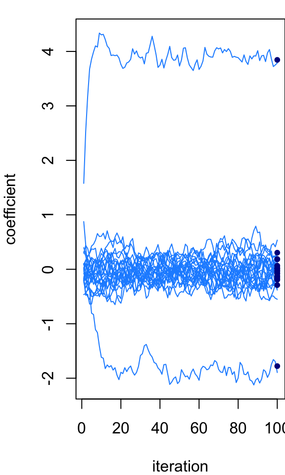
| Version | Author | Date |
|---|---|---|
| 55fe832 | Peter Carbonetto | 2025-03-06 |
At the last iteration, the Markov chain is quite close to the exact posterior mean. But we wouldn’t expect it to be exactly the same because the MCMC is intended to simulate the full posterior distribution, not just recover the posterior mean. However, if we instead take an average of the Markov chain states, then we should (or hopefully) get closer to the exact calculations. This next plot shows the running average across the 100 Gibbs sampler iterations:
par(mar = c(4,4,1,0))
plot_params_over_time(B,show_average = TRUE)
points(rep(niter,p),post$mean,pch = 20,col = "darkblue",cex = 1)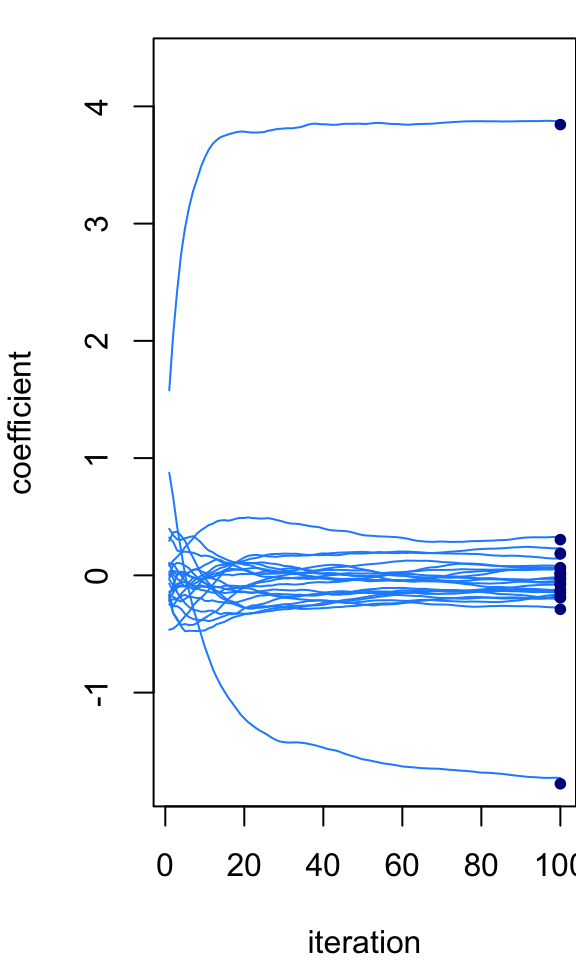
| Version | Author | Date |
|---|---|---|
| 55fe832 | Peter Carbonetto | 2025-03-06 |
A different iterative algorithm
Let’s now consider a different iterative algorithm: on the one hand, like the Gibbs sampler, this new algorithm updates one co-ordinate or dimension at a time; on the other hand, unlike the Gibbs sampler, the updates are deterministic. That is, given the same inputs, this iterative algorithm will always produce the same output. To start, we will simply describe this iterative algorithm, and later we will motivate it as fitting a variational approxiation to the (exact) posterior distribution.
Posterior distribution for the “single-input” ridge regression model
To describe the algorithm, it will be helpful to first write down the posterior distribution for a ridge regression model with a single input (that is, \(p = 1\)), which is a special case of the expressions given above: \[ \bar{b} = \frac{v \mathbf{x}^T\mathbf{y}}{\sigma^2}, \qquad v = \frac{\sigma^2}{\mathbf{x}^T\mathbf{x} + \lambda}. \] For describing the updates, it will be convenient to define these expressions as functions of the data, so let’s change the notation slightly: \[ \bar{b}(\mathbf{x},\mathbf{y}) = \frac{v(\mathbf{x}, \mathbf{y}) \, \mathbf{x}^T\mathbf{y}}{\sigma^2}, \qquad v(\mathbf{x},\mathbf{y}) = \frac{\sigma^2} {\mathbf{x}^T\mathbf{x} + \lambda}. \]
The coordinatewise updates
With these expressions, the coordinatewise updates for the iterative algorithm involve two steps: \[ \begin{aligned} \mathbf{r}_j &\leftarrow \mathbf{y} - \sum_{k\, \neq\, j} \mathbf{x}_k b_k \\ b_j &\leftarrow \bar{b}(\mathbf{x}_j, \mathbf{r}_j). \end{aligned} \] In the machine learning literature, this update are often viewed as “messages” sent between the coordinates and there is a lot of work on studying these algorithms as “message-passing” algorithms.
Let’s now see what these updates look like on the example data set.
The first function here computes the posterior mean and variance for the single-input ridge regression model and the second function is simply a pair of for-loops that repeatedly cycles through the single-coordinate updates for all the \(p\) input variables.
# Return the posterior distribution for the single-input
# ridge regression model given data x, y.
ridge1_post <- function (x, y, s, s0) {
  xx <- sum(x^2)
  xy <- sum(x*y)
  v <- s^2/(xx + (s/s0)^2)
  b <- v*xy/s^2
  return(list(mean = b,var = v))
}

# Perform "niter" updates of the iterative algorithm for ridge
# regression, initialized to "b".
ridge_iterative <- function (X, y, s, s0, niter, b = rep(0,ncol(X))) {
  p <- length(b)
  B <- matrix(0,p,niter)
  for (i in 1:niter) {
    r <- drop(y - X %*% b)
    for (j in 1:p) {
      x <- X[,j]
      r <- r + x*b[j]
      b[j] <- ridge1_post(x,r,s,s0)$mean
      r <- r - x*b[j]
    }
    B[,i] <- b
  }
  return(B)
}
Let’s now run 20 rounds of this updates and look at how the coefficients \(b_j\) change over time:
par(mar = c(4,4,1,0))
niter <- 20
B <- ridge_iterative(X,y,s,s0,niter)
plot_params_over_time(B)
points(rep(niter,p),post$mean,pch = 20,col = "darkblue",cex = 1)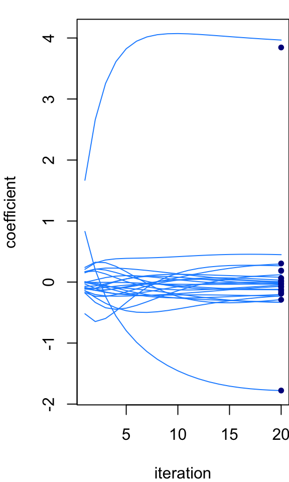
| Version | Author | Date |
|---|---|---|
| 55fe832 | Peter Carbonetto | 2025-03-06 |
Notice that the iterative estimates of the coefficients get progressively closer to the analytical posterior mean. What happens if you run the iterative algorithm longer? Does it ever recover the analytical solution? Do the iterates eventually stop changing (that is, do they “converge” to a fixed point)? Here, we started at an initial estimate where all the coefficients were zero. What happens if we give the algorithm a random starting point?
Discuss differences between this iterative algorithm and the Gibbs sampler. In particular, compare the computational complexity of this iterative algorithm to the Gibbs sampler
Posterior inference as optimization
Posterior inference is fundamentally an integration problem; that is, computing posterior distributions and expectations with respect to the posterior distribution always involves sums or integrals (and sometimes these integrals have known closed-form formulas). The “magic” of variational inference is that it recasts this integration problem as an optimization problem. Here we will see how that happens generally, and for the ridge regression model. The key question we will answer is: what is the objective function we are optimizing?
Note: One possible point of confusion with the ridge expression model is that the posterior mean is also the posterior mode, and as a result the iterative algorithm can also be viewed as an algorithm for finding the posterior mode (i.e., the maximum a posteriori estimate). We will try to avoid this perspective here since our goal is to to illustrate variational inference ideas that could be applicable to other models, not just ridge regression.
The Kullback-Leibler divergence
Let \(q(\mathbf{b})\) denote an approximation to the true posterior \(p_{\mathrm{post}}(\mathbf{b}) = p(\mathbf{b} \mid \mathbf{X}, \mathbf{y})\). The starting point of all variational inference methods is a measure of the difference between the true posterior and the approximation. Here (like most variational inference approaches) we will us the Kullback-Leibler (K-L) divergence measure. The K-L divergence between \(q(\mathbf{b})\) and the posterior is is \[ \mathrm{KL}(q \,\|\, p_{\mathrm{post}}) = \int q(\mathbf{b}) \log \bigg\{\frac{q(\mathbf{b})}{p_{\mathrm{post}}(\mathbf{b})}\bigg\} \, d\mathbf{b}. \] (It is called a “divergence” instead of a “difference” to remind us that this is not a symmetric measure since differences are usually symmetric.)
Smaller “divergences” mean that the two distributions are more similar, and when they are the same, the K-L divergence is zero.
Intuitively, our goal is to find a \(q\) that makes the K-L divergence as small as possible. Therefore, the K-L divergence is the objective we are optimizing (although in practice it isn’t exactly the K-L divergence).
Expanding the terms in the K-L divergence using properties of the logarithm, and expanding out the posterior (Bayes’ Theorem), the K-L divergence works out to \[ \mathrm{KL}(q \,\|\, p_{\mathrm{post}}) = F(q) + \log Z, \] where \[ \begin{aligned} F(q) &= U(q) - H(q) \\ H(q) &= - \textstyle \int q(\mathbf{b}) \log q(\mathbf{b}) \, d\mathbf{b} \\ U(q) &= - \textstyle \int q(\mathbf{b}) \log p(\mathbf{b}) \, d\mathbf{b} \\ Z &= \textstyle \int p(\mathbf{y} \mid \mathbf{X}, \mathbf{b}) \, p(\mathbf{b}) \, d\mathbf{b}. \end{aligned} \] In statistical physics, \(H(q)\) is known as the “entropy”, \(U(q)\) is the “variational average energy” and \(F(q)\) is the “variational free energy”.
Exercise: Derive this result.
Luckily, although \(\log Z\) has an ugly and potentially difficult-to-compute integral inside of it, it does not depend on \(q\), so we can ignore it! In other words, we can equivallently minimize \(F(q)\) (the variational free energy) instead of the K-L divergence. The convention in machine learning is instead to maximize \(-F(q)\), which is called the “Evidence Lower Bound”, or “ELBO”: \[ \mathrm{ELBO}(q) = E_q[\log p(\mathbf{b})] - E_q[\log q(\mathbf{b})]. \] Notice that I’ve rewritten the integrals as expectations. So now are goal is to find a \(q\) that maximizes the ELBO.
Optional exercise: Rewrite all these expressions using expectations instead of integrals.
When \(q(\mathbf{b}) = p_{\mathrm{post}}(\mathbf{b})\), what is the ELBO equal to?
A fully-factorized variational approximation
Recall our goal is to be able to tackle large-scale inference problems. This inevitably requires some sort of compromise: we will have to accept some inaccuracy in the result to achieve faster computations. In variational inference, one can either approximate the ELBO itself, or restrict \(q\) to a distribution that is particularly convenient computationally. One such constraint is that \(q\) factorize into its individual coordinates; that is, \[ q(\mathbf{b}) = \prod_{j=1}^p q_j(b_j). \] In statistical physics, this is called the “mean field” approximation, and is actually an old idea dating back to the 1940s and 1950s. The machine learning community has adopted much of the terminology from statistical physics and so also calls these “mean field” approximations.
Clearly, this approximation will be accurate if the true posterior distribution also factorizes in this way. (Question: when does the ridge regression posterior factorize in this way?) On the other hand, this approximation can be very poor if there are strong correlations among the coordinates. But keep in mind that poor approximations can still (sometimes) be useful!
For some intuition why this approximation is helpful, the hope is that with the property of \(q\) being fully-factorized, the \(p\)-dimensional integrals over \(\mathbf{b}\) will decompose into much lower dimensional integrals, say, in 1 or 2 dimensions, which makes the problem much more tractable. For example, with a fully-factorized \(q\), how does the expectation/integral \(E_q[\mathbf{X} \mathbf{b}]\) decompose into smaller integrals? What is the dimension of those integrals?
Divide and conquer
In summary, our optimization problem is to maximize the ELBO with the constraint that \(q\) is fully-factorized. However it isn’t yet clear how this connects to our iterative algorithm above. The connection is made by taking a “divide and conquer” approach: instead of trying to optimize the entire \(q(\mathbf{b})\) at once, we instead optimize a single coordinate at a to,e, \(q_j(b_j)\). Doing this will lead to the updates given above. This is a very widely used strategy in variational inference and is The proof is a bit tedious and too long to explain in detail here, but it isn’t hard to give a high-level explanation.
Proof sketch:
Work out the expression for the ELBO for the single-input ridge regression model, that is, for the special case when \(p = 1\). Denote this by \(\mathrm{ELBO}^{(p=1)}(q; \mathbf{x}, \mathbf{y})\) to make the dependence of the ELBO on the data explicit.
Next consider the more general (\(p > 1\)) case, but expand only the terms in the ELBO involving \(q_j\). If done carefully, this should give the following result: \[ \mathrm{ELBO}(q) = \mathrm{ELBO}^{(p=1)}(q_j; \mathbf{x}_j, \mathbf{r}_j) + \mathrm{const}, \] in which \(\mathbf{r}_j\) was defined above, and the “const” includes all the terms that do not involve \(q_j\).
In other words, the ELBO can be rearranged to exactly match the expression for the single-input ELBO if we ignore terms not involving \(q_j\). This means that optimizing one coordinate at a time reduces to computing the posterior distribution for a single-input ridge regression model, which is much more manageable than computing the posterior distribution for a ridge regression model with, say, thousands of inputs.
The full derivation of this result is left as an exercise.
By deriving the coordinatewise updates in this way, we have accomplished several things, including:
We can understand the algorithm as an optimization algorithm that is optimizing a specific objective function (the ELBO).
The updates, when they “converge” (stop changing), should (usually) recover a maximum of the ELBO.
We can understand this algorithm as making the approximation that the posterior is fully-factorized. (It turns out that for ridge regression, the posterior means are always exact under this approximation, which is why we saw above that these updates produced coefficients that were very close to the exact posterior means. The variances, on the other hand, which we did not keep track of, do not recover the exact posterior variances.
We can also use the ELBO to monitor progress of the updates.
Connection to EM
Finally, note that the close resemblence of the ELBO to \(F(\theta, q)\) in the vignette on EM is not a coincidence. In fact, this connection has been exploited to develop approximate EM algorithms sometimes called “variational EM”.
Further reading
Blei et al, Variational inference: a review for statisticians.
For a statistical physics perspective, see Yedidia et al, Constructing free-energy approximations and generalized belief propagation algorithms.
Development notes
Some additional important points about variational inference that weren’t well covered in this lesson:
Would be useful to introduce the terminology of “variational parameters”.
The ridge regression example maybe doesn’t drive home that the choice of \(q\) is often approximate (it’s a bit lucky here that the marginals are in fact normal so the choice of \(q\) as normal seems almost like it’s not a choice).
It might be nice to add density or contour plots of the true posterior on two of the betas vs. the same for the variational approximation (similar to Blei’s figure) that would help emphasize how the covariance structure in the posterior is lost.
sessionInfo()R version 4.3.3 (2024-02-29)
Platform: aarch64-apple-darwin20 (64-bit)
Running under: macOS Sonoma 14.7.1
Matrix products: default
BLAS: /Library/Frameworks/R.framework/Versions/4.3-arm64/Resources/lib/libRblas.0.dylib
LAPACK: /Library/Frameworks/R.framework/Versions/4.3-arm64/Resources/lib/libRlapack.dylib; LAPACK version 3.11.0
locale:
[1] en_US.UTF-8/en_US.UTF-8/en_US.UTF-8/C/en_US.UTF-8/en_US.UTF-8
time zone: America/Chicago
tzcode source: internal
attached base packages:
[1] stats graphics grDevices utils datasets methods base
other attached packages:
[1] MASS_7.3-60.0.1
loaded via a namespace (and not attached):
[1] vctrs_0.6.5 cli_3.6.4 knitr_1.45 rlang_1.1.5
[5] xfun_0.42 highr_0.10 stringi_1.8.3 promises_1.2.1
[9] jsonlite_1.8.8 workflowr_1.7.1 glue_1.8.0 rprojroot_2.0.4
[13] git2r_0.33.0 htmltools_0.5.8.1 httpuv_1.6.14 sass_0.4.9
[17] fansi_1.0.6 rmarkdown_2.26 evaluate_0.23 jquerylib_0.1.4
[21] tibble_3.2.1 fastmap_1.1.1 yaml_2.3.8 lifecycle_1.0.4
[25] whisker_0.4.1 stringr_1.5.1 compiler_4.3.3 fs_1.6.5
[29] Rcpp_1.0.12 pkgconfig_2.0.3 later_1.3.2 digest_0.6.34
[33] R6_2.5.1 utf8_1.2.4 pillar_1.9.0 magrittr_2.0.3
[37] bslib_0.6.1 tools_4.3.3 cachem_1.0.8 This site was created with R Markdown