Multivariate normal
Matthew Stephens
University of ChicagoFebruary 10, 2026
Last updated: 2026-02-10
Checks: 7 0
Knit directory: fiveMinuteStats/analysis/
This reproducible R Markdown analysis was created with workflowr (version 1.7.1). The Checks tab describes the reproducibility checks that were applied when the results were created. The Past versions tab lists the development history.
Great! Since the R Markdown file has been committed to the Git repository, you know the exact version of the code that produced these results.
Great job! The global environment was empty. Objects defined in the global environment can affect the analysis in your R Markdown file in unknown ways. For reproduciblity it’s best to always run the code in an empty environment.
The command set.seed(12345) was run prior to running the
code in the R Markdown file. Setting a seed ensures that any results
that rely on randomness, e.g. subsampling or permutations, are
reproducible.
Great job! Recording the operating system, R version, and package versions is critical for reproducibility.
Nice! There were no cached chunks for this analysis, so you can be confident that you successfully produced the results during this run.
Great job! Using relative paths to the files within your workflowr project makes it easier to run your code on other machines.
Great! You are using Git for version control. Tracking code development and connecting the code version to the results is critical for reproducibility.
The results in this page were generated with repository version e92eefb. See the Past versions tab to see a history of the changes made to the R Markdown and HTML files.
Note that you need to be careful to ensure that all relevant files for
the analysis have been committed to Git prior to generating the results
(you can use wflow_publish or
wflow_git_commit). workflowr only checks the R Markdown
file, but you know if there are other scripts or data files that it
depends on. Below is the status of the Git repository when the results
were generated:
Ignored files:
    Ignored:    analysis/bernoulli_poisson_process_cache/
Note that any generated files, e.g. HTML, png, CSS, etc., are not included in this status report because it is ok for generated content to have uncommitted changes.
These are the previous versions of the repository in which changes were
made to the R Markdown (analysis/mvnorm.Rmd) and HTML
(docs/mvnorm.html) files. If you’ve configured a remote Git
repository (see ?wflow_git_remote), click on the hyperlinks
in the table below to view the files as they were in that past version.
| File | Version | Author | Date | Message |
|---|---|---|---|---|
| Rmd | e92eefb | Peter Carbonetto | 2026-02-10 | Generated pdf version of mvnorm vignette. |
| html | 46821ba | Matthew Stephens | 2021-02-28 | Build site. |
| Rmd | 578bfb0 | Matthew Stephens | 2021-02-28 | workflowr::wflow_publish("analysis/mvnorm.Rmd") |
| html | 5f62ee6 | Matthew Stephens | 2019-03-31 | Build site. |
| Rmd | 0cd28bd | Matthew Stephens | 2019-03-31 | workflowr::wflow_publish(all = TRUE) |
| html | 34bcc51 | John Blischak | 2017-03-06 | Build site. |
| Rmd | 5fbc8b5 | John Blischak | 2017-03-06 | Update workflowr project with wflow_update (version 0.4.0). |
| Rmd | 391ba3c | John Blischak | 2017-03-06 | Remove front and end matter of non-standard templates. |
| html | 8e61683 | Marcus Davy | 2017-03-03 | rendered html using wflow_build(all=TRUE) |
| html | 5d0fa13 | Marcus Davy | 2017-03-02 | wflow_build() rendered html files |
| Rmd | d674141 | Marcus Davy | 2017-02-26 | typos, refs |
| html | c3b365a | John Blischak | 2017-01-02 | Build site. |
| Rmd | 67a8575 | John Blischak | 2017-01-02 | Use external chunk to set knitr chunk options. |
| Rmd | 5ec12c7 | John Blischak | 2017-01-02 | Use session-info chunk. |
| Rmd | be2da01 | stephens999 | 2016-02-15 | add multivariate normal |
See here for a PDF version of this vignette.
Prerequisites
You need to know what a univariate normal distribution is, and basic properties such as the fact that linear combinations of normals are also normal. You also need to know the basics of matrix algebra (e.g., matrix multiplication, matrix transpose).
Definition
There are several equivalent ways to define a multivariate normal, but perhaps the most succinct and elegant is this one, which I took from Wikipedia: “a random vector is said to be \(r\)-variate normally distributed if every linear combination of its \(r\) components has a univariate normal distribution”. The special case \(r = 2\) is usually referred to as the “bivariate normal” distribution. And the terminology “\(r\)-dimensional multivariate normal” means the same as \(r\)-variate normal.
Perhaps more insight can be obtained by specifying one way to simulate from a multivariate normal distribution. Suppose \(Z_1, \dots, Z_n\) are independent random variables each with a standard normal distribution \(N(0,1)\). Let \(Z\) denote the vector \((Z_1, \dots, Z_n)\), and let \(A\) be any \(r \times n\) matrix, and \(\mu\) be any \(r\)-vector. Then the vector \(X = AZ + \mu\) has an \(r\)-dimensional multivariate normal distribution with mean \(\mu\) and variance-covariance matrix \(\Sigma := AA^T\). (Here, \(A^T\) means the transpose of the matrix \(A\).) We write \(X \sim N_r(\mu, \Sigma)\).
Note that \(E(X_j) = \mu_j\) and \(\mathrm{Cov}(X_i,X_j) = \Sigma_{ij}\).
When we simulate \(X\) this way, any linear combination of the elements of \(X\) is a linear combination of \(Z\), and so is univariate normal because any linear combination of univariate normals is univariate normal. That is, when we simulate \(X\) this way it satisfies the definition above for being \(r\)-variate normal.
Example
Suppose we define \(X_1 = Z_1 + Z_2\) and \(X_2 = Z_1 + Z_3\) where \(Z_1,Z_2\) and \(Z_3\) are independent standard normal variables. Then \(X = AZ\) where \(A = \begin{pmatrix} 1 & 1 & 0 \\ 1 & 0 & 1 \end{pmatrix}\), and so \(X \sim N_2 (0,\Sigma)\) where \(\Sigma = AA^T = \begin{pmatrix} 2 & 1 \\ 1 & 2 \end{pmatrix}\).
Here is some code to simulate from this distribution:
Z <- rnorm(3)
A <- rbind(c(1,1,0),c(1,0,1))
Sigma <- A %*% t(A)
Sigma
#      [,1] [,2]
# [1,]    2    1
# [2,]    1    2
X <- A %*% Z
And if we want to simulate lots of examples, we can do this lots of times. The following code simulates from this distribution 1m000 times and plots the points.
X <- matrix(0,2,1000)
for(i in 1:1000) {
  Z <- rnorm(3)
  X[,i] <- A %*% Z
}
plot(X[1,],X[2,],main = "bivariate normal",asp = 1,
     xlab = "x1",ylab = "x2",xlim = c(-5,5),ylim = c(-5,5))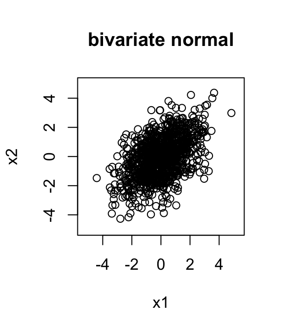
And we can check that the sample covariances are close to the theoretical values:
cov(t(X))
#          [,1]     [,2]
# [1,] 1.844647 0.898902
# [2,] 0.898902 1.915543
General algorithm
From the above, we can see that you can simulate from a multivariate normal with any mean \(\mu\) and variance covariance matrix \(\Sigma\) provided that \(\Sigma\) can be written as \(\Sigma = AA^T\) for some matrix \(A\). This turns out to be possible if and only if \(\Sigma\) is what is known as a “positive semi-definite” matrix—that is, a symmetric matrix with non-negative eigenvalues.
Given a positive semi-definite matrix \(\Sigma\), there are multiple ways to find a
matrix \(A\) such that \(\Sigma = AA^T\) (and indeed multiple
matrices \(A\) that obey this).
However, for our purposes here we only need one way, and here we use the
“Cholesky decomposition”, which finds a unique lower triangular matrix
\(L\) such that \(LL^T =
\Sigma\). Here’s an illustration of the Cholesky decomposition
(the R function chol() finds an upper triangular matrix, so
we transpose it here to make it lower triangular).
Sigma <- rbind(c(2,1),c(1,2))
L <- t(chol(Sigma))
L
#           [,1]     [,2]
# [1,] 1.4142136 0.000000
# [2,] 0.7071068 1.224745
L %*% t(L)
#      [,1] [,2]
# [1,]    2    1
# [2,]    1    2
We can use this to generate any multivariate normal. Here we use it to generate a bivariate normal with covariance matrix \[ \begin{pmatrix} 1.0 & 0.9 \\ 0.9 & 1.0 \end{pmatrix}. \]
my_rmvnorm <- function (mu, Sigma) {
  r <- length(mu)
  L <- t(chol(Sigma))
  Z <- rnorm(r)
  return(L %*% Z + mu)
}
X <- matrix(0,2,1000)
S <- rbind(c(1.0,0.9),c(0.9,1.0))
for (i in 1:1000)
  X[,i] <- my_rmvnorm(c(0,0),S)
plot(X[1,],X[2,],main = " bivariate normal",asp = 1,xlab = "x1",ylab = "x2")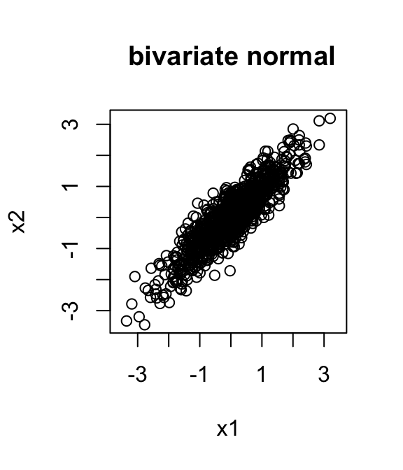
Note: If you want to actually generate multivariate normal random variables in R you should use a more carefully written function like “rmvnorm” from the mvtnorm package.
sessionInfo()
# R version 4.3.3 (2024-02-29)
# Platform: aarch64-apple-darwin20 (64-bit)
# Running under: macOS 15.7.1
#
# Matrix products: default
# BLAS:   /Library/Frameworks/R.framework/Versions/4.3-arm64/Resources/lib/libRblas.0.dylib
# LAPACK: /Library/Frameworks/R.framework/Versions/4.3-arm64/Resources/lib/libRlapack.dylib;  LAPACK version 3.11.0
#
# locale:
# [1] en_US.UTF-8/en_US.UTF-8/en_US.UTF-8/C/en_US.UTF-8/en_US.UTF-8
#
# time zone: America/Chicago
# tzcode source: internal
#
# attached base packages:
# [1] stats     graphics  grDevices utils     datasets  methods   base
#
# loaded via a namespace (and not attached):
#  [1] vctrs_0.6.5       cli_3.6.5         knitr_1.50        rlang_1.1.6
#  [5] xfun_0.52         stringi_1.8.7     promises_1.3.3    jsonlite_2.0.0
#  [9] workflowr_1.7.1   glue_1.8.0        rprojroot_2.0.4   git2r_0.33.0
# [13] htmltools_0.5.8.1 httpuv_1.6.14     sass_0.4.10       rmarkdown_2.29
# [17] evaluate_1.0.4    jquerylib_0.1.4   tibble_3.3.0      fastmap_1.2.0
# [21] yaml_2.3.10       lifecycle_1.0.4   whisker_0.4.1     stringr_1.5.1
# [25] compiler_4.3.3    fs_1.6.6          Rcpp_1.1.0        pkgconfig_2.0.3
# [29] later_1.4.2       digest_0.6.37     R6_2.6.1          pillar_1.11.0
# [33] magrittr_2.0.3    bslib_0.9.0       tools_4.3.3       cachem_1.1.0