Simulating discrete Markov chains: limiting disributions
Matt Bonakdarpour
University of ChicagoJanuary 15, 2026
Last updated: 2026-01-15
Checks: 6 1
Knit directory: fiveMinuteStats/analysis/
This reproducible R Markdown analysis was created with workflowr (version 1.7.1). The Checks tab describes the reproducibility checks that were applied when the results were created. The Past versions tab lists the development history.
The R Markdown file has unstaged changes. To know which version of
the R Markdown file created these results, you’ll want to first commit
it to the Git repo. If you’re still working on the analysis, you can
ignore this warning. When you’re finished, you can run
wflow_publish to commit the R Markdown file and build the
HTML.
Great job! The global environment was empty. Objects defined in the global environment can affect the analysis in your R Markdown file in unknown ways. For reproduciblity it’s best to always run the code in an empty environment.
The command set.seed(12345) was run prior to running the
code in the R Markdown file. Setting a seed ensures that any results
that rely on randomness, e.g. subsampling or permutations, are
reproducible.
Great job! Recording the operating system, R version, and package versions is critical for reproducibility.
Nice! There were no cached chunks for this analysis, so you can be confident that you successfully produced the results during this run.
Great job! Using relative paths to the files within your workflowr project makes it easier to run your code on other machines.
Great! You are using Git for version control. Tracking code development and connecting the code version to the results is critical for reproducibility.
The results in this page were generated with repository version a641c10. See the Past versions tab to see a history of the changes made to the R Markdown and HTML files.
Note that you need to be careful to ensure that all relevant files for
the analysis have been committed to Git prior to generating the results
(you can use wflow_publish or
wflow_git_commit). workflowr only checks the R Markdown
file, but you know if there are other scripts or data files that it
depends on. Below is the status of the Git repository when the results
were generated:
Unstaged changes:
    Modified:   Makefile
    Modified:   analysis/simulating_discrete_chains_1.Rmd
    Modified:   analysis/simulating_discrete_chains_2.Rmd
    Modified:   analysis/stationary_distribution.Rmd
Note that any generated files, e.g. HTML, png, CSS, etc., are not included in this status report because it is ok for generated content to have uncommitted changes.
These are the previous versions of the repository in which changes were
made to the R Markdown
(analysis/simulating_discrete_chains_2.Rmd) and HTML
(docs/simulating_discrete_chains_2.html) files. If you’ve
configured a remote Git repository (see ?wflow_git_remote),
click on the hyperlinks in the table below to view the files as they
were in that past version.
| File | Version | Author | Date | Message |
|---|---|---|---|---|
| html | 5f62ee6 | Matthew Stephens | 2019-03-31 | Build site. |
| Rmd | 0cd28bd | Matthew Stephens | 2019-03-31 | workflowr::wflow_publish(all = TRUE) |
| html | 34bcc51 | John Blischak | 2017-03-06 | Build site. |
| Rmd | 5fbc8b5 | John Blischak | 2017-03-06 | Update workflowr project with wflow_update (version 0.4.0). |
| Rmd | 391ba3c | John Blischak | 2017-03-06 | Remove front and end matter of non-standard templates. |
| html | 8e61683 | Marcus Davy | 2017-03-03 | rendered html using wflow_build(all=TRUE) |
| html | 5d0fa13 | Marcus Davy | 2017-03-02 | wflow_build() rendered html files |
| Rmd | d674141 | Marcus Davy | 2017-02-26 | typos, refs |
| html | c3b365a | John Blischak | 2017-01-02 | Build site. |
| Rmd | 67a8575 | John Blischak | 2017-01-02 | Use external chunk to set knitr chunk options. |
| Rmd | 5ec12c7 | John Blischak | 2017-01-02 | Use session-info chunk. |
| Rmd | f209a9a | mbonakda | 2016-01-30 | fix up typos |
| Rmd | 0f93e3c | mbonakda | 2016-01-30 | split simulating discrete markov chains into three separate notes |
See here for a PDF version of this vignette.
Pre-requisites
This document assumes basic familiarity with simulating Markov chains, as seen here: Simulating Discrete Markov Chains: An Introduction.
Overview
In this note, we show the empirical relationship between the stationary distribution, limiting probabilities, and empirical probabilities for discrete Markov chains.
Limiting Probabilities
Let \(\pi^{(0)}\) be our initial probability vector. For example, if we had a 3 state Markov chain with \(\pi^{(0)} = [0.5, 0.1, 0.4]\), this would tell us that our chain has a 50% probability of starting in state 1, a 10% probability of starting in state 2, and a 40% probability of starting in state 3. If we wanted to have our initial state equal to 1, we would set \(\pi^{(0)} = [1, 0, 0]\).
Let \(P\) be our probability transition matrix. Recall that the probability vector after \(n\) steps is equal to: \[\pi^{(n)} = \pi^{(0)}P^n\] where \(P^n\) is the matrix \(P\) raised to the \(n\)-th power.
With the facts above, we could keep track of our probability vector \(\pi^{(n)}\) as we simulate the Markov chain as follows:
- Obtain probability transition matrix \(P\)
- Set \(P_n = P\)
- For t = 1…T:
- Simulate next step of Markov chain.
- Set \(\pi^{(n)} =
\pi^{(0)}P_n\)
- Set \(P_n = P_nP\)
We augment our function for simulating Markov chains from this note with the
following changes:
1. We keep track of \(\pi^{(n)}\).
2. We add the functionality of simulating multiple chains at once – as a
result, the vectors we dealt with in the previous note have turned into
matrices.
3. We use the rmultinom() function instead of our
inv.transform.sample() method.
# simulate discrete Markov chains
run.mc.sim <- function( P,   # probability transition matrix
                        num.iters=50,
                        num.chains=150 )
  {

  # number of possible states
  num.states <- nrow(P)

  # states X_t for all chains
  states     <- matrix(NA, ncol=num.chains, nrow=num.iters)

  # probability vectors pi^n through time
  all_probs  <- matrix(NA, nrow=num.iters, ncol=num.states)

  # forces chains to start in state 1
  pi_0      <- c(1, rep(0, num.states-1))

  # initialize variables for first state
  P_n           <- P
  all_probs[1,] <- pi_0
  states[1,]    <- 1

  for(t in 2:num.iters) {

    # pi^n for this iteration
    pi_n           <- pi_0 %*% P_n
    all_probs[t,]  <- pi_n

    for(chain_num in seq_len(num.chains)) {
      # probability vector to simulating next state
      p                     <- P[ states[t-1,chain_num], ]
      states[t,chain_num]   <- which(rmultinom(1, 1, p) == 1)
    }

    # update probability transition matrix
    P_n           <- P_n %*% P
  }
  return(list(all.probs=all_probs, states=states))
}
Simulation 1: 3x3 example
Assume our probability transition matrix is: \[P = \begin{bmatrix} 0.7 & 0.2 & 0.1 \\ 0.4 & 0.6 & 0 \\ 0 & 1 & 0 \end{bmatrix}\]
We initialize this matrix in R below:
# setup transition matrix
P <- t(matrix(c( 0.7, 0.2, 0.1,
                 0.4, 0.6,   0,
                   0,   1,   0  ), nrow=3, ncol=3))
We will inspect the limiting probabilities and compare them to the stationary distribution. In this note, we derived the stationary distribution for this transition matrix. Recall that the stationary distribution \(\pi\) is the vector such that \[\pi = \pi P\]
We found that: \[ \pi_1 \approx 0.54, \pi_2 \approx 0.41, \pi_3 \approx 0.05 \]
Therefore, with proper conditions (see below), we expect the Markov chain to spend more time in states 1 and 2 as the chain evolves.
Now we will use the function we wrote in the previous section to check this result numerically.
sim1 <- run.mc.sim(P)Our function returns a list containing two matrices. The second matrix called “states” contains the states of each of our simulated chains through time. Recall that our state space is \(\{1,2,3\}\). Below, we first visualize how 5 of these chains evolve:
states <- sim1[[2]]
matplot(states[,1:5], type='l', lty=1, col=1:5, ylim=c(0,4), ylab='state', xlab='time')
abline(h=1, lty=3)
abline(h=3, lty=3)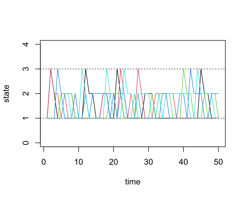
The first matrix we get from our function contains \(\pi^{(n)}\) through time. We can see how \(\pi^{(n)}\) evolves as \(n\) grows, and we can check if it converges to the stationary distribution we found above. For irreducible finite state Markov chains, note that \(\pi^{(n)}\) converges if and only if the Markov chain is aperiodic. In this note, we only consider finite, irreducible, and aperiodic Markov chains.
Using \(\pi^{(n)}\), we plot the time evolution of the probability of being in each state:
all.probs <- sim1[[1]]
matplot(all.probs, type='l', col=1:3, lty=1, ylab='probability', xlab='time')
legend('topright', c('state.1', 'state.2', 'state.3'), lty=1, col=1:3)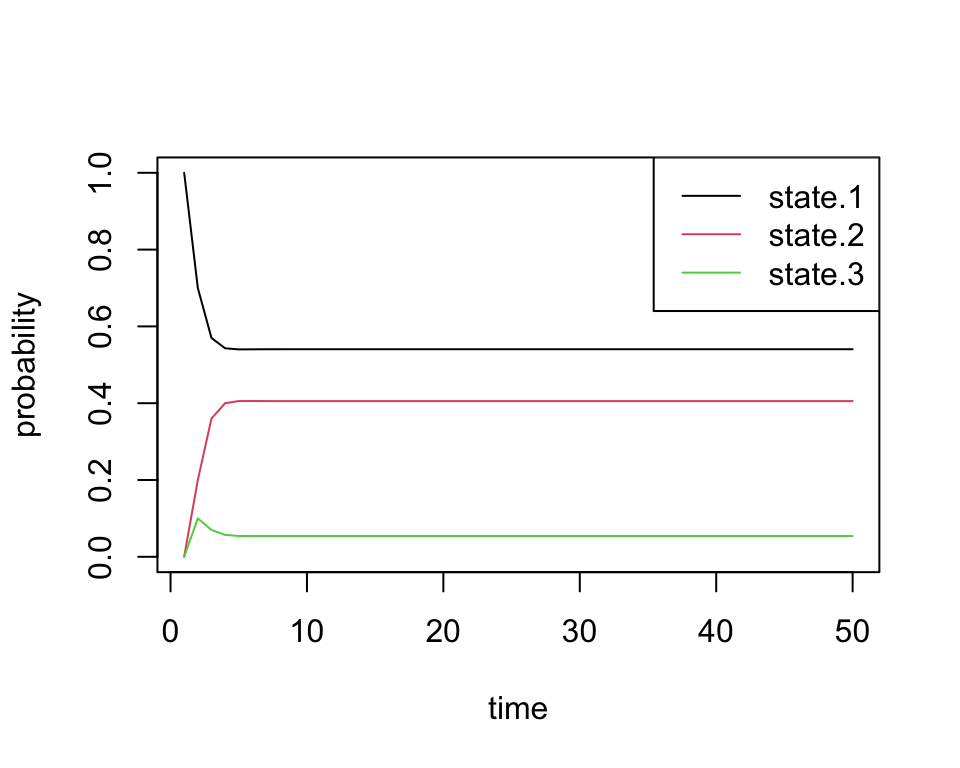
Indeed, we see that these probabilities quickly converge. Just by looking at the plot, we can see that the final probabilities are about equal to the stationary distribution \(\pi\) we found above.
By inspecting the actual values, we confirm that the values of \(\pi^{(n)}\) converge to the vector \(\pi\) exactly. The first row in the matrix below is from the simulation, and the second row is the quantity we obtained by solving for the stationary distribution:
# solve for stationary distribution
A         <- matrix(c(-0.3, 0.2, 0.1, 1, 0.4, -0.4, 0, 1, 0, 1, -1, 1 ), ncol=3,nrow=4)
b         <- c(0,0,0, 1)
pi        <- drop(solve(t(A) %*% A, t(A) %*% b))

# show comparison
results1           <- t(data.frame(pi_n = all.probs[50,], pi = pi))
colnames(results1) <- c('state.1', 'state.2', 'state.3')
results1
#        state.1   state.2    state.3
# pi_n 0.5405405 0.4054054 0.05405405
# pi   0.5405405 0.4054054 0.05405405
Finally, we can also plot the proportion of chains that are in each state through time. These should roughly equal the probability vectors above, with some noise due to random chance:
state.probs <- t(apply(apply(sim1[[2]], 1, function(x) table(factor(x, levels=1:3))), 2, function(x) x/sum(x)))
matplot(state.probs[1:50,], col=1:3, lty=1, type='l', ylab='empirical probability', xlab='time')
legend('topright', c('state.1', 'state.2', 'state.3'), lty=1, col=1:3)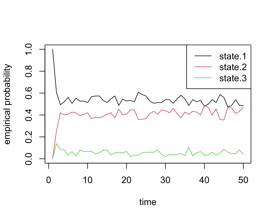
Simulation 2: 8x8 example
Next we will quickly do two larger experiments with the size of our state space equal to 8. Assume our probability transition matrix is: \[P = \begin{bmatrix} 0.33 & 0.66 & 0 & 0 & 0 & 0 & 0 & 0 \\ 0.33 & 0.33 & 0.33 & 0 & 0 & 0 & 0 & 0 \\ 0 & 0.33 & 0.33 & 0.33 & 0 & 0 & 0 & 0 \\ 0 & 0 & 0.33 & 0.33 & 0.33 & 0 & 0 & 0 \\ 0 & 0 & 0 & 0.33 & 0.33 & 0.33 & 0 & 0 \\ 0 & 0 & 0 & 0 & 0.33 & 0.33 & 0.33 & 0 \\ 0 & 0 & 0 & 0 & 0 & 0.33 & 0.33 & 0.33 \\ 0 & 0 & 0 & 0 & 0 & 0 & 0.66 & 0.33 \\ \end{bmatrix}\]
We first initialize our transition matrix in R:
P <- t(matrix(c( 1/3, 2/3,   0,   0,  0,   0,   0,   0,
                 1/3, 1/3, 1/3,   0,  0,   0,   0,   0,
                   0, 1/3, 1/3, 1/3,  0,   0,   0,   0,
                   0,   0, 1/3, 1/3, 1/3,  0,   0,   0,
                   0,   0,   0, 1/3, 1/3, 1/3,  0,   0,
                   0,   0,   0,   0, 1/3, 1/3, 1/3,  0,
                   0,   0,   0,   0,   0, 1/3, 1/3, 1/3,
                   0,   0,   0,   0,   0,   0, 2/3, 1/3), nrow=8, ncol=8))
After briefly studying this matrix, we can see that for states 2 through 7, this transition matrix forces the chain to either stay in the current state or move one state up or down, all with equal probability. For the edge cases, states 1 and 8, the chain can either stay or reflect towards the middle states. Since it’s “easier” to get to one of the middle states (either from above or below), we should see that the probabilities for these states converge to a higher number than the states on the boundaries.
Now we run our simulation with the transition matrix above:
sim2a <- run.mc.sim(P)and now plot 5 of the chains through time below:
states <- sim2a[[2]]
matplot(states[,1:5], type='l', lty=1, col=1:5, ylim=c(0,9), ylab='state', xlab='time')
abline(h=1, lty=3)
abline(h=8, lty=3)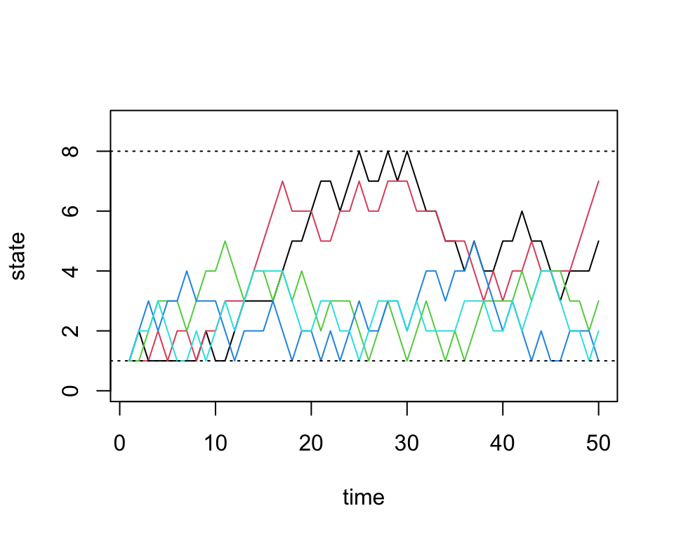
Next we inspect \(\pi^{(n)}\) through time:
all.probs <- sim2a[[1]]
matplot(all.probs, type='l', col=1:8, lty=1, ylab='probability',
        xlab='time', ylim=c(0, 0.5))
legend('topright', paste('state.', 1:8, sep=''), lty=1, col=1:8)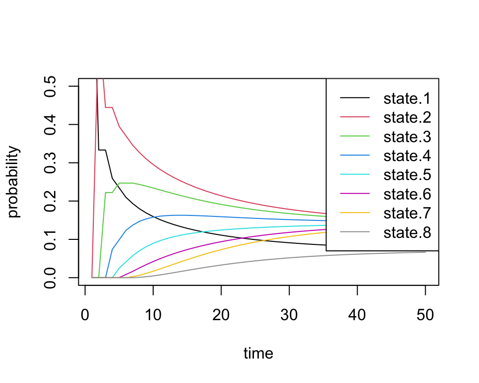
These results match our intuition above. The probability of being in states 1 and 8 converge to smaller values than the others.
Now we alter the transition matrix above to encourage the chain to stay in states 4 and 5: \[P = \begin{bmatrix} 0.33 & 0.66 & 0 & 0 & 0 & 0 & 0 & 0 \\ 0.33 & 0.33 & 0.33 & 0 & 0 & 0 & 0 & 0 \\ 0 & 0.08 & 0.08 & 0.84 & 0 & 0 & 0 & 0 \\ 0 & 0 & 0.08 & 0.84 & 0.08 & 0 & 0 & 0 \\ 0 & 0 & 0 & 0.08 & 0.84 & 0.08 & 0 & 0 \\ 0 & 0 & 0 & 0 & 0.84 & 0.08 & 0.08 & 0 \\ 0 & 0 & 0 & 0 & 0 & 0.33 & 0.33 & 0.33 \\ 0 & 0 & 0 & 0 & 0 & 0 & 0.66 & 0.33 \\ \end{bmatrix}\]
and initialize the transition matrix in R:
P <- t(matrix(c( 1/3,   2/3,    0,    0,    0,    0,    0,   0,
                 1/3,   1/3,  1/3,    0,    0,    0,    0,   0,
                   0,  .5/6, .5/6,  5/6,    0,    0,    0,   0,
                   0,     0, .5/6,  5/6, .5/6,    0,    0,   0,
                   0,     0,    0, .5/6,  5/6, .5/6,    0,   0,
                   0,     0,    0,    0,  5/6, .5/6, .5/6,   0,
                   0,     0,    0,    0,    0,  1/3,  1/3, 1/3,
                   0,     0,    0,    0,    0,    0,  2/3, 1/3 ), nrow=8, ncol=8))
sim2b <- run.mc.sim(P)Below we inspect \(\pi^{(n)}\) through time and see that the probability vector converges to a vector placing most of the probability mass on states 4 and 5.
all.probs <- sim2b[[1]]
matplot(all.probs, type='l', col=1:8, lty=1, ylab='probability',
        xlab='time', ylim=c(0,1.2))
legend('topright', paste('state.', 1:8, sep=''), lty=1, col=1:8)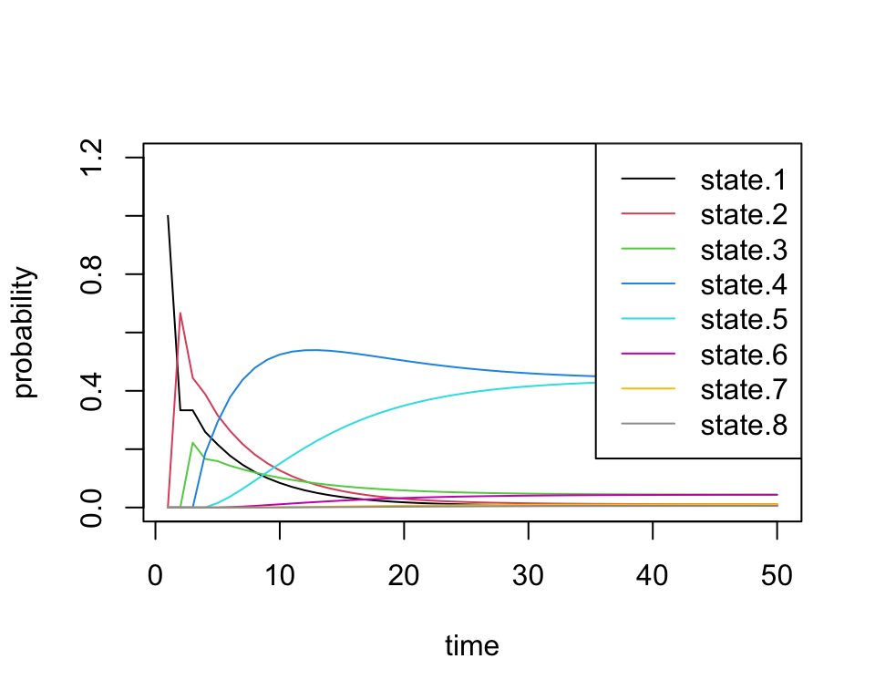
Finally we confirm that our empirical probabilities also exhibit similar behavior:
state.probs <- t(apply(apply(sim2b[[2]], 1, function(x) table(factor(x, levels=1:8))), 2, function(x) x/sum(x)))
matplot(state.probs[1:50,], col=1:8, lty=1, type='l', ylab='empirical probability', xlab='time', ylim=c(0,1.2))
legend('topright', paste('state.', 1:8, sep=''), lty=1, col=1:8)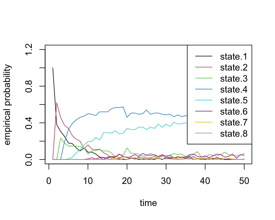
sessionInfo()
# R version 4.3.3 (2024-02-29)
# Platform: aarch64-apple-darwin20 (64-bit)
# Running under: macOS 15.7.1
#
# Matrix products: default
# BLAS:   /Library/Frameworks/R.framework/Versions/4.3-arm64/Resources/lib/libRblas.0.dylib
# LAPACK: /Library/Frameworks/R.framework/Versions/4.3-arm64/Resources/lib/libRlapack.dylib;  LAPACK version 3.11.0
#
# locale:
# [1] en_US.UTF-8/en_US.UTF-8/en_US.UTF-8/C/en_US.UTF-8/en_US.UTF-8
#
# time zone: America/Chicago
# tzcode source: internal
#
# attached base packages:
# [1] stats     graphics  grDevices utils     datasets  methods   base
#
# loaded via a namespace (and not attached):
#  [1] vctrs_0.6.5       cli_3.6.5         knitr_1.50        rlang_1.1.6
#  [5] xfun_0.52         stringi_1.8.7     promises_1.3.3    jsonlite_2.0.0
#  [9] workflowr_1.7.1   glue_1.8.0        rprojroot_2.0.4   git2r_0.33.0
# [13] htmltools_0.5.8.1 httpuv_1.6.14     sass_0.4.10       rmarkdown_2.29
# [17] evaluate_1.0.4    jquerylib_0.1.4   tibble_3.3.0      fastmap_1.2.0
# [21] yaml_2.3.10       lifecycle_1.0.4   whisker_0.4.1     stringr_1.5.1
# [25] compiler_4.3.3    fs_1.6.6          Rcpp_1.1.0        pkgconfig_2.0.3
# [29] later_1.4.2       digest_0.6.37     R6_2.6.1          pillar_1.11.0
# [33] magrittr_2.0.3    bslib_0.9.0       tools_4.3.3       cachem_1.1.0