The likelihood function
Matthew Stephens
University of ChicagoJanuary 12, 2026
Last updated: 2026-01-12
Checks: 7 0
Knit directory: fiveMinuteStats/analysis/
This reproducible R Markdown analysis was created with workflowr (version 1.7.1). The Checks tab describes the reproducibility checks that were applied when the results were created. The Past versions tab lists the development history.
Great! Since the R Markdown file has been committed to the Git repository, you know the exact version of the code that produced these results.
Great job! The global environment was empty. Objects defined in the global environment can affect the analysis in your R Markdown file in unknown ways. For reproduciblity it’s best to always run the code in an empty environment.
The command set.seed(12345) was run prior to running the
code in the R Markdown file. Setting a seed ensures that any results
that rely on randomness, e.g. subsampling or permutations, are
reproducible.
Great job! Recording the operating system, R version, and package versions is critical for reproducibility.
Nice! There were no cached chunks for this analysis, so you can be confident that you successfully produced the results during this run.
Great job! Using relative paths to the files within your workflowr project makes it easier to run your code on other machines.
Great! You are using Git for version control. Tracking code development and connecting the code version to the results is critical for reproducibility.
The results in this page were generated with repository version 4c61063. See the Past versions tab to see a history of the changes made to the R Markdown and HTML files.
Note that you need to be careful to ensure that all relevant files for
the analysis have been committed to Git prior to generating the results
(you can use wflow_publish or
wflow_git_commit). workflowr only checks the R Markdown
file, but you know if there are other scripts or data files that it
depends on. Below is the status of the Git repository when the results
were generated:
working directory clean
Note that any generated files, e.g. HTML, png, CSS, etc., are not included in this status report because it is ok for generated content to have uncommitted changes.
These are the previous versions of the repository in which changes were
made to the R Markdown (analysis/likelihood_function.Rmd)
and HTML (docs/likelihood_function.html) files. If you’ve
configured a remote Git repository (see ?wflow_git_remote),
click on the hyperlinks in the table below to view the files as they
were in that past version.
| File | Version | Author | Date | Message |
|---|---|---|---|---|
| Rmd | 4c61063 | Peter Carbonetto | 2026-01-12 | Some minor updates to the likelihood_function vignette. |
| html | a221240 | Peter Carbonetto | 2026-01-09 | Push a bunch of updates to the webpages. |
| Rmd | 25e1cf5 | Peter Carbonetto | 2026-01-08 | Adding pdf versions of three other vignettes. |
| html | 5f62ee6 | Matthew Stephens | 2019-03-31 | Build site. |
| Rmd | 0cd28bd | Matthew Stephens | 2019-03-31 | workflowr::wflow_publish(all = TRUE) |
| html | 34bcc51 | John Blischak | 2017-03-06 | Build site. |
| Rmd | 5fbc8b5 | John Blischak | 2017-03-06 | Update workflowr project with wflow_update (version 0.4.0). |
| Rmd | 391ba3c | John Blischak | 2017-03-06 | Remove front and end matter of non-standard templates. |
| html | 8e61683 | Marcus Davy | 2017-03-03 | rendered html using wflow_build(all=TRUE) |
| html | 5d0fa13 | Marcus Davy | 2017-03-02 | wflow_build() rendered html files |
| Rmd | d674141 | Marcus Davy | 2017-02-26 | typos, refs |
| html | c3b365a | John Blischak | 2017-01-02 | Build site. |
| Rmd | 67a8575 | John Blischak | 2017-01-02 | Use external chunk to set knitr chunk options. |
| Rmd | 5ec12c7 | John Blischak | 2017-01-02 | Use session-info chunk. |
| Rmd | 506f3b9 | stephens999 | 2016-04-06 | updates |
| Rmd | e140df9 | stephens999 | 2016-04-06 | correct bug |
| Rmd | 8354ea5 | stephens999 | 2016-04-06 | correct some typos |
| Rmd | 3ee2cf4 | stephens999 | 2016-01-12 | add likelihood function |
See here for a PDF version of this vignette.
Prerequisites
You should understand the concept of using likelihood ratio for discrete data and continuous data to compare support for two fully specified models.
Overview
We have seen how one can use the likelihood ratio to compare the support in the data for two fully-specified models. In practice, we often want to compare more than two models — indeed, we often want to compare a continuum of models. This is where the idea of a likelihood function comes from.
Example
In the example here, we assumed that the frequencies of different alleles (genetic types) in forest and savanna elephants were given to us. In practice, these frequencies themselves would have to be estimated from data.
For example, suppose we collect data on 100 savanna elephants, and we see that 30 of them carry allele 1 at marker 1, and 70 carry the allele 0 at marker 1 (again we are treating elephants as haploid to simplify things). Intuitively, we might estimate that the frequency of the 1 allele at that marker is 30/100, or 0.3. But we might think that the data are also consistent with other frequencies near 0.3. For example, maybe the data are also consistent with a frequency of 0.29. Or 0.28? Or…
In this case, we have many more than just two models to compare. Indeed, if we allow that the frequency could, in principle, lie anywhere in the interval [0,1], then we have a continuum of models to compare.
Specifically, for each \(q\in [0,1]\), let \(M_q\) denote the model that the true frequency of the 1 allele is \(q\). Then, given our observation that 30 of 100 elephants carry allele 1 at marker 1, the likelihood for model \(M_q\) is, by the previous definition, \[ L(M_q) = \Pr(D \mid M_q) = q^{30} (1-q)^{70}. \] And the LR comparing models \(M_{q_1}\) and \(M_{q_2}\) is \[ \mathrm{LR}(M_{q_1}, M_{q_2}) = [q_1/q_2]^{30} [(1-q_1)/(1-q_2)]^{70}. \]
This is an example of what is called a parametric model. A parametric model is collection of models indexed by a parameter vector, often denoted \(\theta\), whose values lie in some parameter space, usually denoted \(\Theta\). The number of parameters included in the vector \(\theta\) is called the “dimensionality” of the model or parameter space, and often denoted \(\mathrm{dim}(\Theta)\).
Here the parameter is \(q\), and the parameter space is \([0,1]\). The dimensionality of the parameter space is 1.
When computing likelihoods for parametric models, we usually dispense with the model notation and simply use the parameter value to denote the model. So instead of referring to the likelihood for \(M_q\) we just say the “likelihood for \(q\)”, and write \(L(q)\). So the likelihood for \(q\) is given by \[ L(q) = q^{30} (1-q)^{70}. \] Correspondingly, we can also refer to the “likelihood ratio for \(q_1\) vs. \(q_2\)”.
We could plot the likelihood function as follows:
q <- seq(0,1,length.out = 100)
L <- function (q)
  q^30 * (1-q)^70
plot(q,L(q),ylab = "L(q)",xlab = "q",type = "l")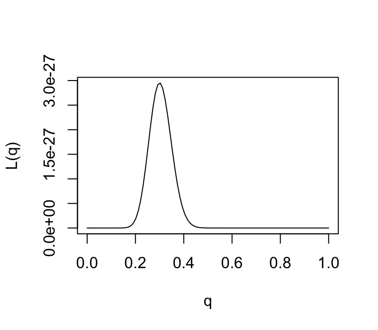
The value of \(\theta\) that maximizes the likelihood function is referred to as the “maximum likelihood estimate”, and usually denoted \(\hat{\theta}\). That is, \[ \hat{\theta} := \underset{\theta \,\in\, \Theta}{\mathrm{argmax}} \, L(\theta). \]
Provided the data are sufficiently informative and the number of parameters is not too large, maximum likelihood estimates tend to be sensible. In this case, we can see that the maximum likelihood estimate is \(q = 0.3\), which corresponds to our intuition.
Note that from the likelihood function we can easily compute the likelihood ratio for any pair of parameter values! And just as with comparing two models, it is not the likelihoods that matter, but the likelihood ratios. That is, you can divide the likelihood function by any constant without affecting the likelihood ratios.
One way to emphasize this is to standardize the likelihood function so that its maximum is at 1, by dividing \(L(\theta)/L(\hat{\theta})\).
q <- seq(0,1,length.out = 100)
L <- function (q)
  q^30 * (1-q)^70
plot(q,L(q)/L(0.3),ylab = "L(q)/L(qhat)",xlab = "q",type = "l")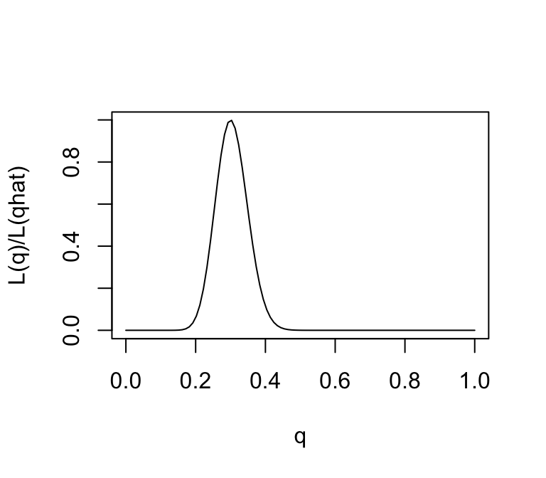
Note that, for some values of \(q\), the likelihood ratio compared with \(q=0.3\) is very close to zero. These values of \(q\) are so much less consistent with the data that they are effectively excluded by the data. Just looking at the picture we might say that the values of \(q\) less than 0.15 or bigger than 0.5 are pretty much excluded by the data. We will see later how Bayesian analysis methods can be used to make this kind of argument more formal.
The log-likelihood
Just as it can often be convenient to work with the log-likelihood ratio, it can be convenient to work with the log-likelihood function, usually denoted \(l(\theta)\) (“lowercase L”). As with log-likelihood ratios, unless otherwise specified, we use the “base e” log. Here is the log-likelihood function:
q <- seq(0,1,length.out = 100)
l <- function (q)
  30*log(q) + 70 * log(1-q)
plot(q,l(q) - l(0.3),ylab = "l(q) - l(qhat)",xlab = "q",type = "l",
     ylim = c(-10,0))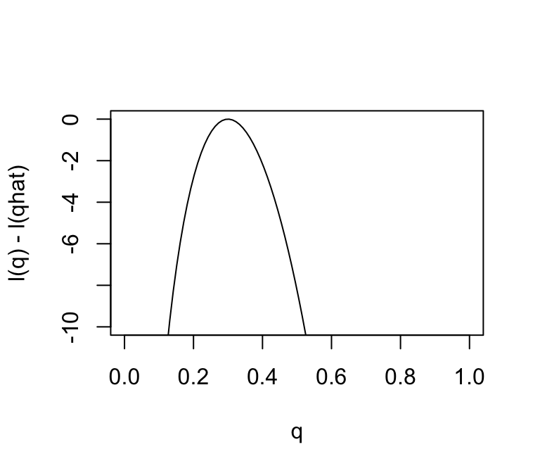
Changes in the log-likelihood function are referred to as “log-likelihood units”. For example, the difference in the support for \(q = 0.3\) and \(q = 0.35\) is \(l(0.3) - l(0.35)\) which is 0.5630377 log-likelihood units. Again, remember that it is differences in \(l\) that matter.
Notice that the scale of the Y axis in this plot was set to span 10 log-likelihood units. Setting the scale in this way makes sure the plot focuses on the parts of the parameter space that have more than minuscule support from the data (in this case, LR no smaller than \(1/e^{10}\). Without this, the plot can be much harder to read. For example, here is the plot using the default scale selected by R:
plot(q,l(q) - l(0.3),ylab = "l(q) - l(qhat)",xlab = "q",type = "l")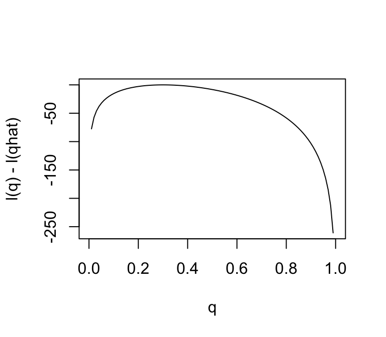
Notice how different this plot looks to the eye even though it is exactly the same curve being plotted (just different Y axis scale). It is worth thinking about what scale you use when plotting log-likelihoods (and, of course, figures in general!).
sessionInfo()
# R version 4.3.3 (2024-02-29)
# Platform: aarch64-apple-darwin20 (64-bit)
# Running under: macOS 15.7.1
#
# Matrix products: default
# BLAS:   /Library/Frameworks/R.framework/Versions/4.3-arm64/Resources/lib/libRblas.0.dylib
# LAPACK: /Library/Frameworks/R.framework/Versions/4.3-arm64/Resources/lib/libRlapack.dylib;  LAPACK version 3.11.0
#
# locale:
# [1] en_US.UTF-8/en_US.UTF-8/en_US.UTF-8/C/en_US.UTF-8/en_US.UTF-8
#
# time zone: America/Chicago
# tzcode source: internal
#
# attached base packages:
# [1] stats     graphics  grDevices utils     datasets  methods   base
#
# loaded via a namespace (and not attached):
#  [1] vctrs_0.6.5       cli_3.6.5         knitr_1.50        rlang_1.1.6
#  [5] xfun_0.52         stringi_1.8.7     promises_1.3.3    jsonlite_2.0.0
#  [9] workflowr_1.7.1   glue_1.8.0        rprojroot_2.0.4   git2r_0.33.0
# [13] htmltools_0.5.8.1 httpuv_1.6.14     sass_0.4.10       rmarkdown_2.29
# [17] evaluate_1.0.4    jquerylib_0.1.4   tibble_3.3.0      fastmap_1.2.0
# [21] yaml_2.3.10       lifecycle_1.0.4   whisker_0.4.1     stringr_1.5.1
# [25] compiler_4.3.3    fs_1.6.6          Rcpp_1.1.0        pkgconfig_2.0.3
# [29] later_1.4.2       digest_0.6.37     R6_2.6.1          pillar_1.11.0
# [33] magrittr_2.0.3    bslib_0.9.0       tools_4.3.3       cachem_1.1.0