FGF Nuclei Neuron Prep
Last updated: 2019-10-28
Checks: 6 1
Knit directory: fgf_alldata/
This reproducible R Markdown analysis was created with workflowr (version 1.4.0). The Checks tab describes the reproducibility checks that were applied when the results were created. The Past versions tab lists the development history.
Great! Since the R Markdown file has been committed to the Git repository, you know the exact version of the code that produced these results.
The global environment had objects present when the code in the R Markdown file was run. These objects can affect the analysis in your R Markdown file in unknown ways. For reproduciblity it’s best to always run the code in an empty environment. Use wflow_publish or wflow_build to ensure that the code is always run in an empty environment.
The following objects were defined in the global environment when these results were created:
| Name | Class | Size |
|---|---|---|
| data | environment | 56 bytes |
| env | environment | 56 bytes |
The command set.seed(20191021) was run prior to running the code in the R Markdown file. Setting a seed ensures that any results that rely on randomness, e.g. subsampling or permutations, are reproducible.
Great job! Recording the operating system, R version, and package versions is critical for reproducibility.
Nice! There were no cached chunks for this analysis, so you can be confident that you successfully produced the results during this run.
Great job! Using relative paths to the files within your workflowr project makes it easier to run your code on other machines.
Great! You are using Git for version control. Tracking code development and connecting the code version to the results is critical for reproducibility. The version displayed above was the version of the Git repository at the time these results were generated.
Note that you need to be careful to ensure that all relevant files for the analysis have been committed to Git prior to generating the results (you can use wflow_publish or wflow_git_commit). workflowr only checks the R Markdown file, but you know if there are other scripts or data files that it depends on. Below is the status of the Git repository when the results were generated:
Ignored files:
    Ignored:    .Rproj.user/
    Ignored:    test_files/

Untracked files:
    Untracked:  code/sc_functions.R
    Untracked:  data/fgf_filtered_nuclei.RDS
    Untracked:  data/filtglia.RDS
    Untracked:  data/glia/
    Untracked:  data/lps1.txt
    Untracked:  data/mcao1.txt
    Untracked:  data/mcao_d3.txt
    Untracked:  data/mcaod7.txt
    Untracked:  data/neur_astro_induce.xlsx
    Untracked:  data/neuron/
    Untracked:  data/synaptic_activity_induced.xlsx
    Untracked:  docs/figure/
    Untracked:  olig_ttest_padj.csv
    Untracked:  output/agrp_pcgenes.csv
    Untracked:  output/all_wc_markers.csv
    Untracked:  output/allglia_wgcna_genemodules.csv
    Untracked:  output/glia/
    Untracked:  output/glial_markergenes.csv
    Untracked:  output/integrated_all_markergenes.csv
    Untracked:  output/integrated_neuronmarkers.csv
    Untracked:  output/neuron/
Note that any generated files, e.g. HTML, png, CSS, etc., are not included in this status report because it is ok for generated content to have uncommitted changes.
There are no past versions. Publish this analysis with wflow_publish() to start tracking its development.
Load Libraries
library(Seurat)
library(tidyverse)
library(DESeq2)
library(here)
library(future)
library(cluster)
library(parallelDist)
library(ggplot2)
library(cowplot)
plan("multiprocess", workers = 16)
options(future.globals.maxSize = 4000 * 1024^2)
Functions
source(here("code/sc_functions.R"))Load prepped data
seur.sub<-readRDS(here("data/fgf_filtered_nuclei.RDS"))
a <- DimPlot(seur.sub, reduction="tsne", label=T)+ theme_void() + NoLegend()
Warning: Using `as.character()` on a quosure is deprecated as of rlang 0.3.0.
Please use `as_label()` or `as_name()` instead.
This warning is displayed once per session.b <- DimPlot(seur.sub, reduction="tsne", group.by = "group") + theme_void()
plot_grid(a,b, rel_widths = c(1,1.5))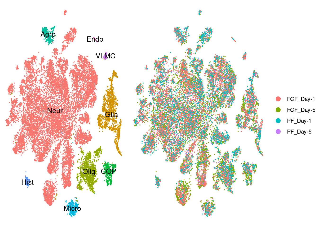
Subset Neurons and Recluster
fgf.neur<-subset(seur.sub, ident=c("Agrp","Neur","Hist"))
# Run the standard workflow for visualization and clustering
fgf.neur %>% ScaleData(verbose = TRUE,block.size = 15000) %>%
  RunPCA(verbose = FALSE) %>%
  RunUMAP(dims = 1:30) %>%
  FindNeighbors(dims = 1:30) %>%
  FindClusters(resolution=0.1) -> fgf.neur
Modularity Optimizer version 1.3.0 by Ludo Waltman and Nees Jan van Eck
Number of nodes: 19416
Number of edges: 1033519
Running Louvain algorithm...
Maximum modularity in 10 random starts: 0.9599
Number of communities: 13
Elapsed time: 3 secondsDimPlot(fgf.neur, label=T)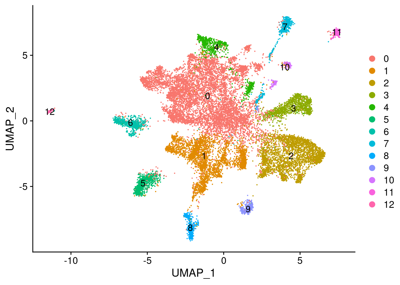
Silhouette calculation and removal of doublets/poor quality cells
fgf.neur<-RunSIL(fgf.neur, ndims = 30)
fgf.neur.sub<-subset(fgf.neur, subset= silhouette>0)
Check which cells are removed
cellrem<-data.frame(sil=ifelse(fgf.neur$silhouette>0, yes="T", no="F"), sample=fgf.neur$sample,
                    trt=fgf.neur$trt, day=fgf.neur$day,cell_type=as.character(Idents(fgf.neur)))
cellrem%>%group_by(sample)%>%
  dplyr::count(sil)%>%ggplot(aes(x=sample, y=n, fill=sil)) +
  geom_bar(position = "fill",stat = "identity")  + ylab("Percent of Cells") + xlab(NULL) + theme(legend.position = "none", axis.text.x = element_text(angle=45, hjust=1)) -> p1
cellrem%>%group_by(day)%>%
  dplyr::count(sil)%>%ggplot(aes(x=day, y=n, fill=sil)) +
  geom_bar(position = "fill",stat = "identity") + theme(legend.position = "none") +ylab(NULL) + xlab(NULL) -> p2
cellrem%>%group_by(cell_type)%>%
  dplyr::count(sil)%>%ggplot(aes(x=cell_type, y=n, fill=sil)) +
  geom_bar(position = "fill",stat = "identity") + scale_fill_discrete(name = "Cell\nKept?") + ylab(NULL) + xlab(NULL) + theme(axis.text.x = element_text(angle=45, hjust=1)) -> p3
plot_grid(p1,p2,p3, nrow=1, axis="b", align = "hv")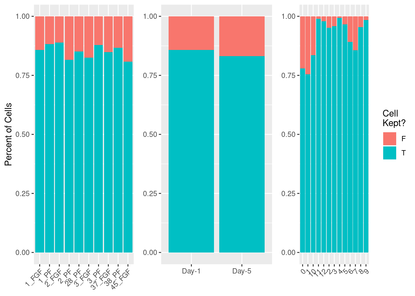
Run the standard workflow for visualization and clustering
fgf.neur.sub %>% ScaleData(verbose = TRUE,block.size = 15000) %>%
  RunPCA(verbose = FALSE) %>%
  RunTSNE(dims = 1:30) -> fgf.neur.sub
Identify marker genes
DefaultAssay(fgf.neur.sub)<-"SCT"
marks<-FindAllMarkers(fgf.neur.sub, only.pos = T, logfc.threshold = .5, max.cells.per.ident = 100)
write_csv(marks, path=here("output/integrated_neuronmarkers.csv"))
marks%>%group_by(cluster)%>%top_n(5, avg_logFC)%>%data.frame->top5
DoHeatmap(fgf.neur.sub, top5$gene)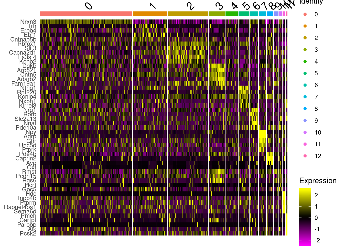
Identify clusters for silhouette removal of poor quality cells
new.cluster.ids<-c("Nrxn3","Trh","Rbfox1","Arpp21","Unknown", "Ntng1",
             "Rorb", "Agrp", "Avp/Oxt", "Rmst", "Hcrt","Hdc","Pmch")
names(new.cluster.ids) <- levels(fgf.neur.sub)
fgf.neur.sub <- RenameIdents(fgf.neur.sub, new.cluster.ids)
DimPlot(fgf.neur.sub, reduction="tsne", label=T)
Save final neuron object
saveRDS(fgf.neur.sub, here("data/neuron/neurons_seur_filtered.RDS"))
sessionInfo()R version 3.5.3 (2019-03-11)
Platform: x86_64-pc-linux-gnu (64-bit)
Running under: Storage
Matrix products: default
BLAS/LAPACK: /usr/lib64/libopenblas-r0.3.3.so
locale:
[1] LC_CTYPE=en_DK.UTF-8 LC_NUMERIC=C
[3] LC_TIME=en_DK.UTF-8 LC_COLLATE=en_DK.UTF-8
[5] LC_MONETARY=en_DK.UTF-8 LC_MESSAGES=en_DK.UTF-8
[7] LC_PAPER=en_DK.UTF-8 LC_NAME=C
[9] LC_ADDRESS=C LC_TELEPHONE=C
[11] LC_MEASUREMENT=en_DK.UTF-8 LC_IDENTIFICATION=C
attached base packages:
[1] parallel stats4 stats graphics grDevices utils datasets
[8] methods base
other attached packages:
[1] cowplot_1.0.0 parallelDist_0.2.4
[3] cluster_2.1.0 future_1.14.0
[5] here_0.1 DESeq2_1.22.2
[7] SummarizedExperiment_1.12.0 DelayedArray_0.8.0
[9] BiocParallel_1.16.6 matrixStats_0.54.0
[11] Biobase_2.42.0 GenomicRanges_1.34.0
[13] GenomeInfoDb_1.18.2 IRanges_2.16.0
[15] S4Vectors_0.20.1 BiocGenerics_0.28.0
[17] forcats_0.4.0 stringr_1.4.0
[19] dplyr_0.8.3 purrr_0.3.2
[21] readr_1.3.1.9000 tidyr_0.8.3
[23] tibble_2.1.3 ggplot2_3.2.1
[25] tidyverse_1.2.1 Seurat_3.0.3.9036
loaded via a namespace (and not attached):
[1] reticulate_1.13 R.utils_2.9.0 tidyselect_0.2.5
[4] RSQLite_2.1.1 AnnotationDbi_1.44.0 htmlwidgets_1.3
[7] grid_3.5.3 Rtsne_0.15 munsell_0.5.0
[10] codetools_0.2-16 ica_1.0-2 withr_2.1.2
[13] colorspace_1.4-1 highr_0.8 knitr_1.23
[16] rstudioapi_0.10 ROCR_1.0-7 gbRd_0.4-11
[19] listenv_0.7.0 labeling_0.3 Rdpack_0.11-0
[22] git2r_0.25.2 GenomeInfoDbData_1.2.0 bit64_0.9-7
[25] rprojroot_1.3-2 vctrs_0.2.0 generics_0.0.2
[28] xfun_0.8 R6_2.4.0 rsvd_1.0.2
[31] locfit_1.5-9.1 bitops_1.0-6 assertthat_0.2.1
[34] SDMTools_1.1-221.1 scales_1.0.0 nnet_7.3-12
[37] gtable_0.3.0 npsurv_0.4-0 globals_0.12.4
[40] workflowr_1.4.0 rlang_0.4.0 zeallot_0.1.0
[43] genefilter_1.64.0 splines_3.5.3 lazyeval_0.2.2
[46] acepack_1.4.1 broom_0.5.2 checkmate_1.9.4
[49] yaml_2.2.0 reshape2_1.4.3 modelr_0.1.4
[52] backports_1.1.4 Hmisc_4.2-0 tools_3.5.3
[55] gplots_3.0.1.1 RColorBrewer_1.1-2 ggridges_0.5.1
[58] Rcpp_1.0.2 plyr_1.8.4 base64enc_0.1-3
[61] zlibbioc_1.28.0 RCurl_1.95-4.12 rpart_4.1-15
[64] pbapply_1.4-1 zoo_1.8-6 haven_2.1.0
[67] ggrepel_0.8.1 fs_1.3.1 magrittr_1.5
[70] RSpectra_0.15-0 data.table_1.12.2 lmtest_0.9-37
[73] RANN_2.6.1 fitdistrplus_1.0-14 hms_0.5.0
[76] lsei_1.2-0 evaluate_0.14 xtable_1.8-4
[79] XML_3.98-1.20 readxl_1.3.1 gridExtra_2.3
[82] compiler_3.5.3 KernSmooth_2.23-15 crayon_1.3.4
[85] R.oo_1.22.0 htmltools_0.3.6 Formula_1.2-3
[88] geneplotter_1.60.0 RcppParallel_4.4.3 lubridate_1.7.4
[91] DBI_1.0.0 MASS_7.3-51.4 Matrix_1.2-17
[94] cli_1.1.0 R.methodsS3_1.7.1 gdata_2.18.0
[97] metap_1.1 igraph_1.2.4.1 pkgconfig_2.0.2
[100] foreign_0.8-71 plotly_4.9.0 xml2_1.2.0
[103] annotate_1.60.1 XVector_0.22.0 bibtex_0.4.2
[106] rvest_0.3.4 digest_0.6.20 sctransform_0.2.0
[109] RcppAnnoy_0.0.12 tsne_0.1-3 rmarkdown_1.13
[112] cellranger_1.1.0 leiden_0.3.1 htmlTable_1.13.1
[115] uwot_0.1.3 gtools_3.8.1 nlme_3.1-140
[118] jsonlite_1.6 viridisLite_0.3.0 pillar_1.4.2
[121] lattice_0.20-38 httr_1.4.1 survival_2.44-1.1
[124] glue_1.3.1 png_0.1-7 bit_1.1-14
[127] stringi_1.4.3 blob_1.1.1 latticeExtra_0.6-28
[130] caTools_1.17.1.2 memoise_1.1.0 irlba_2.3.3
[133] future.apply_1.3.0 ape_5.3