Last updated: 2019-10-28

Checks: 6 1

Knit directory: fgf_alldata/

This reproducible R Markdown analysis was created with workflowr (version 1.4.0). The Checks tab describes the reproducibility checks that were applied when the results were created. The Past versions tab lists the development history.

R Markdown file: up-to-date

Great! Since the R Markdown file has been committed to the Git repository, you know the exact version of the code that produced these results.

Environment: objects present

The global environment had objects present when the code in the R Markdown file was run. These objects can affect the analysis in your R Markdown file in unknown ways. For reproduciblity it’s best to always run the code in an empty environment. Use wflow_publish or wflow_build to ensure that the code is always run in an empty environment.

The following objects were defined in the global environment when these results were created:

Name	Class	Size
data	environment	56 bytes
env	environment	56 bytes

Seed: set.seed(20191021)

The command set.seed(20191021) was run prior to running the code in the R Markdown file. Setting a seed ensures that any results that rely on randomness, e.g. subsampling or permutations, are reproducible.

Session information: recorded

Great job! Recording the operating system, R version, and package versions is critical for reproducibility.

Cache: none

Nice! There were no cached chunks for this analysis, so you can be confident that you successfully produced the results during this run.

File paths: relative

Great job! Using relative paths to the files within your workflowr project makes it easier to run your code on other machines.

Repository version: a4ac5aa

Great! You are using Git for version control. Tracking code development and connecting the code version to the results is critical for reproducibility. The version displayed above was the version of the Git repository at the time these results were generated.

Note that you need to be careful to ensure that all relevant files for the analysis have been committed to Git prior to generating the results (you can use wflow_publish or wflow_git_commit). workflowr only checks the R Markdown file, but you know if there are other scripts or data files that it depends on. Below is the status of the Git repository when the results were generated:


Ignored files:
    Ignored:    .Rproj.user/
    Ignored:    test_files/

Untracked files:
    Untracked:  code/sc_functions.R
    Untracked:  data/fgf_filtered_nuclei.RDS
    Untracked:  data/filtglia.RDS
    Untracked:  data/glia/
    Untracked:  data/lps1.txt
    Untracked:  data/mcao1.txt
    Untracked:  data/mcao_d3.txt
    Untracked:  data/mcaod7.txt
    Untracked:  data/neur_astro_induce.xlsx
    Untracked:  data/neuron/
    Untracked:  data/synaptic_activity_induced.xlsx
    Untracked:  docs/figure/
    Untracked:  olig_ttest_padj.csv
    Untracked:  output/agrp_pcgenes.csv
    Untracked:  output/all_wc_markers.csv
    Untracked:  output/allglia_wgcna_genemodules.csv
    Untracked:  output/glia/
    Untracked:  output/glial_markergenes.csv
    Untracked:  output/integrated_all_markergenes.csv
    Untracked:  output/integrated_neuronmarkers.csv
    Untracked:  output/neuron/

Unstaged changes:
    Modified:   analysis/8_astro_wgcna.Rmd

Note that any generated files, e.g. HTML, png, CSS, etc., are not included in this status report because it is ok for generated content to have uncommitted changes.

There are no past versions. Publish this analysis with wflow_publish() to start tracking its development.

library(Seurat)
library(tidyverse)
library(gProfileR)
library(ggraph)
library(future)
library(org.Mm.eg.db)
library(reactome.db)
library(ggraph)
library(igraph)
library(DESeq2)
library(here)
library(tidyverse)
library(ggrepel)
library(ggpubr)
library(wesanderson)
library(tidygraph)
library(ggforce)
library(reshape2)
library(ggbeeswarm)
library(ggsci)
library(cowplot)
library(gt)
plan(multiprocess, workers=16)
options(future.globals.maxSize = 4000 * 1024^2)

Load prepped data

fgf.neur.sub<-readRDS(here("data/neuron/neurons_seur_filtered.RDS"))

Specific Agrp analysis

agrp<-subset(fgf.neur.sub, ident="Agrp")
agrp %>% ScaleData(verbose=F) %>% 
  FindVariableFeatures(selection.method = "vst", nfeatures = 2000) %>%
  RunPCA(ndims.print=1:10)->agrp
list_sub<-SplitObject(agrp, split.by="sample")
pb<-(lapply(list_sub, function(y) {
    DefaultAssay(y) <- "SCT"
    mat<-GetAssayData(y, slot="counts")
    counts <- Matrix::rowSums(mat)
}) %>% do.call(rbind, .) %>% t() %>% as.data.frame())

trt<-ifelse(grepl("FGF", colnames(pb)), yes="F", no="P")
batch<-as.factor(sapply(strsplit(colnames(pb),"_"),"[",1))
day<-ifelse(as.numeric(as.character(batch))>10, yes="Day-5", no="Day-1")
group<-paste0(trt,"_",day)
meta<-data.frame(trt=trt, day=factor(day), group=group)
dds <- DESeqDataSetFromMatrix(countData = pb,
                              colData = meta,
                              design = ~ 0 + group)
keep <- rowSums(counts(dds) >= 5) > 5
dds <- dds[keep,]
dds<-DESeq(dds)
res_5<-results(dds, contrast = c("group","F_Day-5","P_Day-5"))
res_1<-results(dds, contrast = c("group","F_Day-1","P_Day-1"))
f_5_1<-results(dds, contrast = c("group","F_Day-5","F_Day-1"))
p_5_1<-results(dds, contrast = c("group","P_Day-5","P_Day-1"))

Filter 24 hr results

res_1<-as.data.frame(res_1)
res_1<-res_1[complete.cases(res_1),]
res_1<-res_1[order(res_1$padj),]
res_1$gene<-rownames(res_1)
write_csv(res_1, path=here("output/neuron/agrp_24hr_dge.csv"))

Volcano Plot of DE genes

res_1 %>% add_rownames("gene") %>%
  mutate(siglog=ifelse(padj<0.05&abs(log2FoldChange)>1, yes=T, no=F)) %>% 
  mutate(onlysig=ifelse(padj<0.05&abs(log2FoldChange)<1, yes=T, no=F)) %>% 
  mutate(onlylog=ifelse(padj>0.05&abs(log2FoldChange)>1, yes=T, no=F)) %>% 
  mutate(col=ifelse(siglog==T, yes="1", no = 
                      ifelse(onlysig==T, yes="2", no = 
                               ifelse(onlylog==T, yes="3", no="4")))) %>% 
  mutate(label=ifelse(padj<0.01, yes=gene, no="")) %>%
  dplyr::select(gene, log2FoldChange, padj, col, label) -> volc

Warning: Deprecated, use tibble::rownames_to_column() instead.

ggplot(volc, aes(y=(-log10(padj)), x=log2FoldChange, fill=factor(col), label=label)) + 
  xlab(expression(Log[2]*~Fold*~Change)) + ylab(expression(-Log[10]*~pvalue))+
  geom_point(shape=21, size=3, alpha=0.75) + geom_hline(yintercept = -log10(0.05), linetype="dashed") + 
  geom_vline(xintercept = c(-1,1), linetype="dashed") + geom_text_repel() + theme_pubr() + labs_pubr() + 
  theme(legend.position = "none") + 
  scale_fill_manual(values = wes_palette("Royal1", 4, type="discrete"))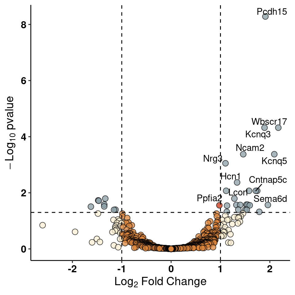

GO Term Analysis

resgo<-res_1[res_1$padj<0.1,]
resgo<-resgo[resgo$log2FoldChange>0,]

ego<-gprofiler(rownames(resgo), organism = "mmusculus", significant = T, custom_bg = rownames(dds),
                           src_filter = c("GO:BP","GO:MF","REAC","KEGG"),hier_filtering = "strong",
                           min_isect_size = 3, 
                           sort_by_structure = T,exclude_iea = T, 
                           min_set_size = 10, max_set_size = 300,correction_method = "fdr")
write_csv(ego, path=here("output/neuron/agrp_24hr_goterms.csv"))

ego %>% arrange(p.value) %>%
  select(domain, term.name, p.value) %>% 
  head(10) %>%
  gt()

domain	term.name	p.value
BP	regulation of membrane potential	0.000773
MF	voltage-gated cation channel activity	0.001780
BP	inorganic cation transmembrane transport	0.002580
BP	animal organ morphogenesis	0.008260
BP	multicellular organism growth	0.011000
BP	cellular response to nitrogen compound	0.014400
BP	regulation of long-term synaptic potentiation	0.020600
rea	Neuronal System	0.023700
BP	transmembrane receptor protein tyrosine kinase signaling pathway	0.029900
BP	synapse organization	0.031300

GO similarity plot

mouse.GO <- as.data.frame(org.Mm.egGO2ALLEGS)[,c("gene_id","go_id")]
mouse.PATH <- as.data.frame(org.Mm.egPATH2EG)[,c("gene_id","path_id")]
mouse.PATH$path_id<-paste0("KEGG:",mouse.PATH$path_id)
mouse.REAC <- as.data.frame(reactomePATHID2EXTID)[,c("gene_id","DB_ID")]
colnames(mouse.REAC)[2]<-"path_id"
mouse.REAC$path_id<-paste0("REAC:",mouse.REAC$path_id)
colnames(mouse.GO)[2]<-"path_id"
allpaths<-rbind(mouse.GO, mouse.PATH)
jac<-allpaths[allpaths$path_id%in%ego$term.id,]
jac_list<-split(jac$gene_id, f = jac$path_id)
df<-stringdist::seq_distmatrix(jac_list,method="jw")
attributes(df)$Labels<-ego[match(attributes(df)$Labels, ego$term.id),"term.name"]

g<-graph.adjacency(
  as.matrix(df),
  mode="undirected",
  weighted=TRUE,
  diag=T)

g<-delete_edges(g,which(E(g)$weight>.6))
g<-as_tbl_graph(g)
g %>% activate(nodes) %>%
  mutate(db = factor(toupper(ego[match(name, ego$term.name),"domain"]))) %>% 
  mutate(pval = -log10(ego[match(name, ego$term.name),"p.value"])) -> g

g %>% activate(nodes) %>% 
  mutate(community = as.factor(group_edge_betweenness())) %>% group_by(community) %>%
  mutate(label=ifelse(pval==max(pval),name, NA)) -> g

set.seed("139")
ggraph(g, layout = "fr") + 
  geom_edge_link(color="black", aes(width = weight), alpha = 0.2, show.legend = F)  + 
  scale_edge_width(range = c(0.2, 1)) + 
  geom_node_point(aes(size=pval, colour=db)) + scale_size(range = c(2,10)) + guides(colour = guide_legend(override.aes = list(size = 5))) +
  geom_mark_hull(aes(x=x,y=y, fill=community), show.legend = F)  + 
  geom_label_repel(aes(x=x,y=y,label=str_wrap(label,20)),fontface="bold", size=4, min.segment.length = .1, nudge_y = .5, alpha=0.5) +
  labs(colour="Database", size=expression(log[10]*pvalue)) + 
  theme_graph()

Warning: Removed 7 rows containing missing values (geom_label_repel).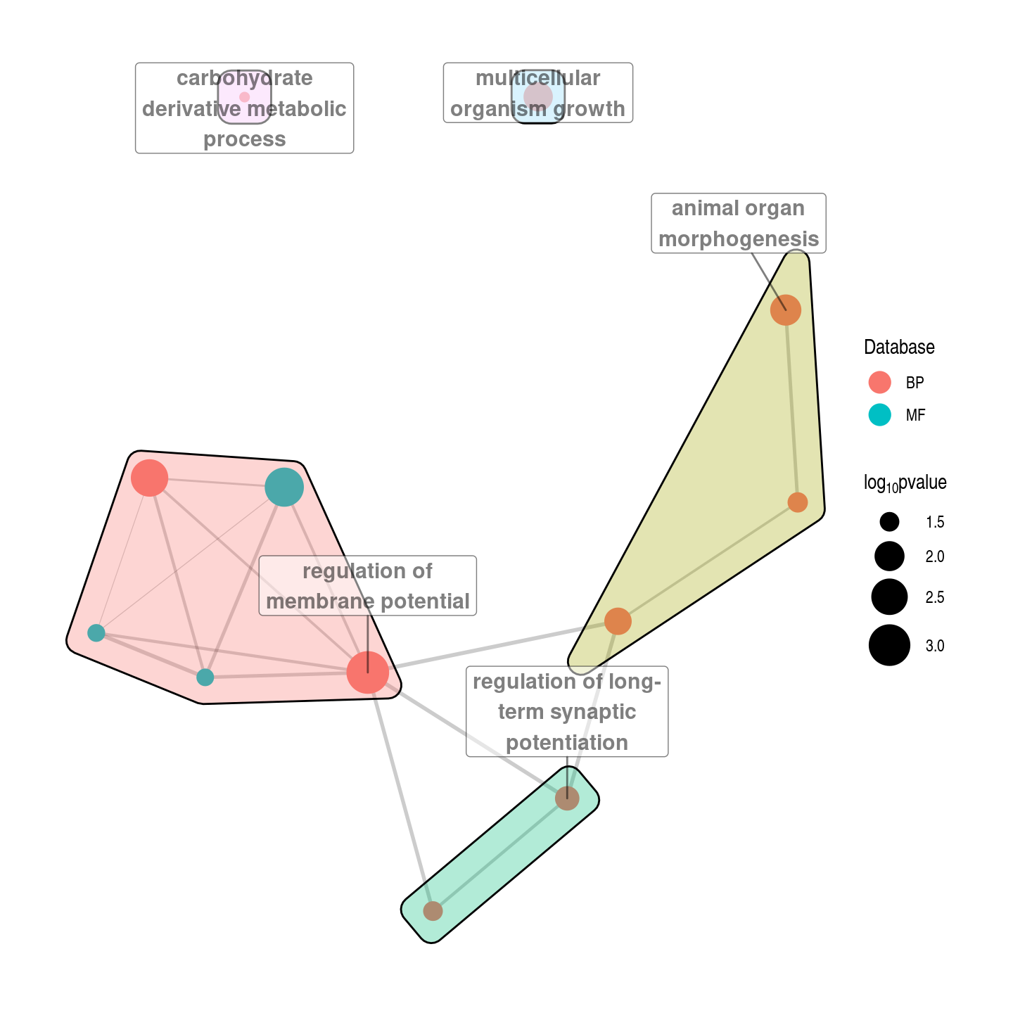

ggsave(filename = here("output/neuron/agrp_go_graph.png"))

Warning: Removed 7 rows containing missing values (geom_label_repel).

D5 v D1

embed <- data.frame(Embeddings(agrp, reduction = "pca")[,1:10])
embed$group <- agrp$group
embed <- melt(embed, id.vars = "group")
ggplot(embed[embed$variable%in%c("PC_1","PC_2","PC_3","PC_4","PC_5","PC_6"),], aes(x = group, y=value)) + 
  geom_quasirandom(aes(fill=group), alpha=.5, shape=21) + 
  facet_wrap(.~variable, scales="free") +
  scale_fill_jco()  + theme_pubr() + 
  theme(legend.position = "none", axis.text.x = element_text(angle=45, hjust=1)) + 
  ylab("PC Embedding Value") + xlab(NULL) + labs_pubr()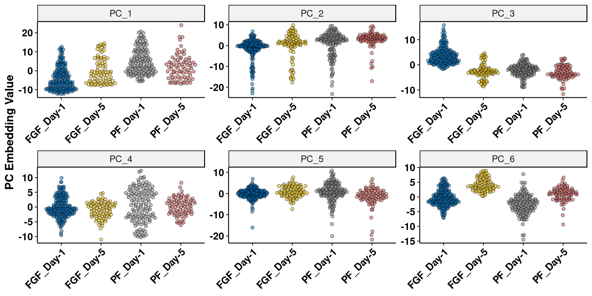

ggsave(filename = here("output/neuron/agrp_pc_graph.png"))

Calculate Variance Explained

mat <- Seurat::GetAssayData(agrp, assay = "SCT", slot = "scale.data")
pca <- agrp[["pca"]]
# Get the total variance:
total_variance <- sum(matrixStats::rowVars(mat))
eigValues = Stdev(object = agrp, reduction = "pca")^2
varExplained = eigValues / total_variance

Extract genes from top loading PCs

pc1<-rownames(agrp@reductions$pca[order(agrp@reductions$pca[,1]),])[1:100]
pc4<-rownames(agrp@reductions$pca[order(-agrp@reductions$pca[,4]),])[1:100]
pc6<-rownames(agrp@reductions$pca[order(-agrp@reductions$pca[,6]),])[1:100]
imp_pcs<-data.frame(pc1=rownames(agrp@reductions$pca[order(agrp@reductions$pca[,1]),]), pc4=rownames(agrp@reductions$pca[order(-agrp@reductions$pca[,4]),]),pc6=rownames(agrp@reductions$pca[order(-agrp@reductions$pca[,6]),]))
write_csv(imp_pcs, path=here("output/agrp_pcgenes.csv"))

res_5<-as.data.frame(res_5)
res_5<-res_5[complete.cases(res_5),]
res_5[order(res_5$pvalue),] %>% add_rownames("gene") %>% filter(baseMean>100)

Warning: Deprecated, use tibble::rownames_to_column() instead.

# A tibble: 92 x 7
   gene    baseMean log2FoldChange lfcSE  stat   pvalue  padj
   <chr>      <dbl>          <dbl> <dbl> <dbl>    <dbl> <dbl>
 1 Cntn5       173.          1.74  0.487  3.57 0.000354 0.883
 2 Mylip       233.         -1.47  0.527 -2.79 0.00523  1.000
 3 Pcdh15      147.          1.06  0.383  2.77 0.00563  1.000
 4 Nlgn1       181.          0.850 0.349  2.44 0.0148   1.000
 5 Pcdh7       194.          0.925 0.400  2.31 0.0208   1.000
 6 Galntl6     142.          0.912 0.408  2.24 0.0254   1.000
 7 Nrg1        157.          0.773 0.375  2.06 0.0392   1.000
 8 Lrrtm4      167.          0.860 0.449  1.92 0.0554   1.000
 9 Npy        1264.         -1.33  0.716 -1.85 0.0643   1.000
10 Syt1        103.          0.761 0.421  1.81 0.0708   1.000
# … with 82 more rows

GO term enrichment for PC6 (highest value for FGF_D5)

pc6_go<-gprofiler(pc6, organism = "mmusculus", significant = T, 
                           src_filter = c("GO:BP","GO:MF","REAC", "KEGG"),hier_filtering = "strong",
                           min_isect_size = 3, 
                           sort_by_structure = T,exclude_iea = T, 
                           min_set_size = 10, max_set_size = 500,correction_method = "fdr")

write_csv(pc6_go, path=here("output/neuron/agrp_PC6_goterms.csv"))
pc6_go %>% arrange(p.value) %>%
  select(domain, term.name, p.value) %>% 
  head(10) %>%
  gt()

domain	term.name	p.value
rea	Neuronal System	2.59e-06
BP	forebrain development	1.14e-04
BP	regulation of transmembrane transport	1.02e-03
BP	presynaptic membrane organization	1.02e-03
BP	cell-cell adhesion via plasma-membrane adhesion molecules	2.07e-03
BP	positive regulation of neurogenesis	2.41e-03
BP	cellular potassium ion transport	2.41e-03
BP	regulation of cell morphogenesis	4.47e-03
keg	Gap junction	4.72e-03
BP	negative regulation of JAK-STAT cascade	4.78e-03

Plot top loading genes

imp_gene<-data.frame(t(agrp[["SCT"]]@scale.data[c("Agrp","Npy","Cntn5"),]))
imp_gene$group<-agrp$group
imp_gene$Sample<-agrp$sample
imp_gene<-melt(imp_gene, id.vars = c("group","Sample"))
ggplot(imp_gene[sample(nrow(imp_gene)),], aes(x=group, y=value)) + 
  geom_quasirandom(aes(fill=Sample),alpha=.85, shape=21) +
  facet_wrap(.~variable, scales = "free", nrow = 1) + theme_pubr() + 
  theme(axis.text.x = element_text(angle=45, hjust=1), legend.position = "right") + 
  ylab("Normalized Expression") + xlab(NULL) + labs_pubr()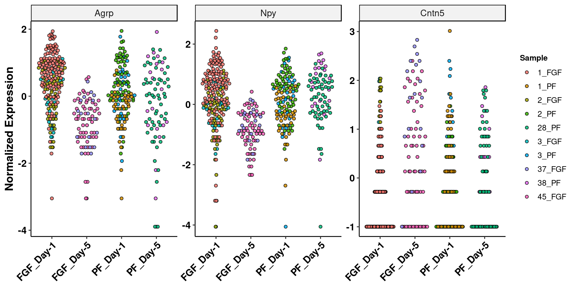

ggsave(filename = here("output/neuron/agrp_imp_gene.png"))

sessionInfo()

R version 3.5.3 (2019-03-11)
Platform: x86_64-pc-linux-gnu (64-bit)
Running under: Storage

Matrix products: default
BLAS/LAPACK: /usr/lib64/libopenblas-r0.3.3.so

locale:
 [1] LC_CTYPE=en_DK.UTF-8       LC_NUMERIC=C              
 [3] LC_TIME=en_DK.UTF-8        LC_COLLATE=en_DK.UTF-8    
 [5] LC_MONETARY=en_DK.UTF-8    LC_MESSAGES=en_DK.UTF-8   
 [7] LC_PAPER=en_DK.UTF-8       LC_NAME=C                 
 [9] LC_ADDRESS=C               LC_TELEPHONE=C            
[11] LC_MEASUREMENT=en_DK.UTF-8 LC_IDENTIFICATION=C       

attached base packages:
[1] parallel  stats4    stats     graphics  grDevices utils     datasets 
[8] methods   base     

other attached packages:
 [1] gt_0.1.0                    cowplot_1.0.0              
 [3] ggsci_2.9                   ggbeeswarm_0.6.0           
 [5] reshape2_1.4.3              ggforce_0.3.0.9000         
 [7] tidygraph_1.1.2             wesanderson_0.3.6.9000     
 [9] ggpubr_0.2.1                magrittr_1.5               
[11] ggrepel_0.8.1               here_0.1                   
[13] DESeq2_1.22.2               SummarizedExperiment_1.12.0
[15] DelayedArray_0.8.0          BiocParallel_1.16.6        
[17] matrixStats_0.54.0          GenomicRanges_1.34.0       
[19] GenomeInfoDb_1.18.2         igraph_1.2.4.1             
[21] reactome.db_1.66.0          org.Mm.eg.db_3.7.0         
[23] AnnotationDbi_1.44.0        IRanges_2.16.0             
[25] S4Vectors_0.20.1            Biobase_2.42.0             
[27] BiocGenerics_0.28.0         future_1.14.0              
[29] ggraph_1.0.2                gProfileR_0.6.7            
[31] forcats_0.4.0               stringr_1.4.0              
[33] dplyr_0.8.3                 purrr_0.3.2                
[35] readr_1.3.1.9000            tidyr_0.8.3                
[37] tibble_2.1.3                ggplot2_3.2.1              
[39] tidyverse_1.2.1             Seurat_3.0.3.9036          

loaded via a namespace (and not attached):
  [1] utf8_1.1.4             reticulate_1.13        R.utils_2.9.0         
  [4] tidyselect_0.2.5       RSQLite_2.1.1          htmlwidgets_1.3       
  [7] grid_3.5.3             Rtsne_0.15             munsell_0.5.0         
 [10] codetools_0.2-16       ica_1.0-2              withr_2.1.2           
 [13] colorspace_1.4-1       highr_0.8              knitr_1.23            
 [16] rstudioapi_0.10        ROCR_1.0-7             ggsignif_0.5.0        
 [19] gbRd_0.4-11            listenv_0.7.0          labeling_0.3          
 [22] Rdpack_0.11-0          git2r_0.25.2           GenomeInfoDbData_1.2.0
 [25] polyclip_1.10-0        bit64_0.9-7            farver_1.1.0          
 [28] rprojroot_1.3-2        vctrs_0.2.0            generics_0.0.2        
 [31] xfun_0.8               R6_2.4.0               rsvd_1.0.2            
 [34] locfit_1.5-9.1         concaveman_1.0.0       bitops_1.0-6          
 [37] assertthat_0.2.1       SDMTools_1.1-221.1     scales_1.0.0          
 [40] nnet_7.3-12            beeswarm_0.2.3         gtable_0.3.0          
 [43] npsurv_0.4-0           globals_0.12.4         workflowr_1.4.0       
 [46] rlang_0.4.0            genefilter_1.64.0      zeallot_0.1.0         
 [49] splines_3.5.3          lazyeval_0.2.2         acepack_1.4.1         
 [52] checkmate_1.9.4        broom_0.5.2            yaml_2.2.0            
 [55] modelr_0.1.4           backports_1.1.4        Hmisc_4.2-0           
 [58] tools_3.5.3            gplots_3.0.1.1         RColorBrewer_1.1-2    
 [61] ggridges_0.5.1         Rcpp_1.0.2             plyr_1.8.4            
 [64] base64enc_0.1-3        zlibbioc_1.28.0        RCurl_1.95-4.12       
 [67] rpart_4.1-15           pbapply_1.4-1          viridis_0.5.1         
 [70] zoo_1.8-6              haven_2.1.0            cluster_2.1.0         
 [73] fs_1.3.1               data.table_1.12.2      lmtest_0.9-37         
 [76] RANN_2.6.1             fitdistrplus_1.0-14    xtable_1.8-4          
 [79] hms_0.5.0              lsei_1.2-0             evaluate_0.14         
 [82] XML_3.98-1.20          readxl_1.3.1           gridExtra_2.3         
 [85] compiler_3.5.3         V8_2.3                 KernSmooth_2.23-15    
 [88] crayon_1.3.4           R.oo_1.22.0            htmltools_0.3.6       
 [91] Formula_1.2-3          geneplotter_1.60.0     RcppParallel_4.4.3    
 [94] lubridate_1.7.4        DBI_1.0.0              tweenr_1.0.1          
 [97] MASS_7.3-51.4          Matrix_1.2-17          cli_1.1.0             
[100] R.methodsS3_1.7.1      gdata_2.18.0           metap_1.1             
[103] pkgconfig_2.0.2        foreign_0.8-71         plotly_4.9.0          
[106] xml2_1.2.0             annotate_1.60.1        vipor_0.4.5           
[109] stringdist_0.9.5.2     XVector_0.22.0         bibtex_0.4.2          
[112] rvest_0.3.4            digest_0.6.20          sctransform_0.2.0     
[115] RcppAnnoy_0.0.12       tsne_0.1-3             rmarkdown_1.13        
[118] cellranger_1.1.0       leiden_0.3.1           htmlTable_1.13.1      
[121] uwot_0.1.3             curl_4.0               gtools_3.8.1          
[124] nlme_3.1-140           jsonlite_1.6           fansi_0.4.0           
[127] viridisLite_0.3.0      pillar_1.4.2           lattice_0.20-38       
[130] httr_1.4.1             survival_2.44-1.1      glue_1.3.1            
[133] png_0.1-7              bit_1.1-14             sass_0.1.2.1          
[136] stringi_1.4.3          blob_1.1.1             latticeExtra_0.6-28   
[139] caTools_1.17.1.2       memoise_1.1.0          irlba_2.3.3           
[142] future.apply_1.3.0     ape_5.3

Agrp_Analysis