GO enrichment
Philipp Bayer
01/10/2021
Last updated: 2021-10-18
Checks: 7 0
Knit directory: Amphibolis_Posidonia_Comparison/
This reproducible R Markdown analysis was created with workflowr (version 1.6.2). The Checks tab describes the reproducibility checks that were applied when the results were created. The Past versions tab lists the development history.
Great! Since the R Markdown file has been committed to the Git repository, you know the exact version of the code that produced these results.
Great job! The global environment was empty. Objects defined in the global environment can affect the analysis in your R Markdown file in unknown ways. For reproduciblity it’s best to always run the code in an empty environment.
The command set.seed(20210414) was run prior to running the code in the R Markdown file. Setting a seed ensures that any results that rely on randomness, e.g. subsampling or permutations, are reproducible.
Great job! Recording the operating system, R version, and package versions is critical for reproducibility.
Nice! There were no cached chunks for this analysis, so you can be confident that you successfully produced the results during this run.
Great job! Using relative paths to the files within your workflowr project makes it easier to run your code on other machines.
Great! You are using Git for version control. Tracking code development and connecting the code version to the results is critical for reproducibility.
The results in this page were generated with repository version 35aa72f. See the Past versions tab to see a history of the changes made to the R Markdown and HTML files.
Note that you need to be careful to ensure that all relevant files for the analysis have been committed to Git prior to generating the results (you can use wflow_publish or wflow_git_commit). workflowr only checks the R Markdown file, but you know if there are other scripts or data files that it depends on. Below is the status of the Git repository when the results were generated:
Ignored files:
    Ignored:    .Rhistory
    Ignored:    .Rproj.user/
    Ignored:    analysis/OTT.nb.html
    Ignored:    analysis/plotGenes.nb.html
    Ignored:    analysis/plotRgenes.nb.html
Note that any generated files, e.g. HTML, png, CSS, etc., are not included in this status report because it is ok for generated content to have uncommitted changes.
These are the previous versions of the repository in which changes were made to the R Markdown (analysis/GOenrichment.Rmd) and HTML (docs/GOenrichment.html) files. If you’ve configured a remote Git repository (see ?wflow_git_remote), click on the hyperlinks in the table below to view the files as they were in that past version.
| File | Version | Author | Date | Message |
|---|---|---|---|---|
| Rmd | 35aa72f | Philipp Bayer | 2021-10-18 | wflow_publish(c("analysis/GOenrichment.Rmd", "analysis/plotGenes.Rmd", |
| Rmd | 7e370e9 | Philipp Bayer | 2021-10-07 | Updated GOenrichment |
| Rmd | 95586f9 | Philipp Bayer | 2021-10-07 | Add missing data |
| html | 95586f9 | Philipp Bayer | 2021-10-07 | Add missing data |
| html | c0db4a5 | Philipp Bayer | 2021-10-07 | Build site. |
| Rmd | 08b28ea | Philipp Bayer | 2021-10-07 | wflow_publish(files = c("analysis/*")) |
Lost in seagrasses
The GO enrichment does not work well on my laptop so I’m setting this to eval=FALSE and run it on a remote server. The script which writes the input files is a Python script in the scripts/ folder: findClustersUniqueToAquatic.py. This script parses Orthofinder output to pull out genome-specific groups and genes.
# give properly formatted background in format: GO:0005838  GSBRNA2T00088508001;GSBRNA2T00088313001;GSBRNA2T00035842001
#annAT <- readMappings('BACKGROUND.txt.gz', sep="\t", IDsep=";")
#save(annAT, file='annAtObject.RData')

load('annAtObject.RData')
allgenes <- unique(unlist(annAT))

compare <- function(genelistfile, outname, allgenes, annAT) {
  # give file with your genes of interest, one gene_id per line

  mygenes <-scan(genelistfile ,what="")
  geneList <- factor(as.integer(allgenes %in% mygenes))
  names(geneList) <- allgenes

  GOdata <-new ("topGOdata", ontology = 'BP', allGenes = geneList, nodeSize = 5, annot=annFUN.GO2genes, GO2genes=annAT)
  # using ClassicCount:
  #test.stat <-new ("classicCount", testStatistic = GOFisherTest, name = "Fisher Test")
  #resultsFisherC <-getSigGroups (GOdata, test.stat)
  # using weight01:
  weight01.fisher <- runTest(GOdata, statistic = "fisher")
  # using ClassicCount:
  # allRes <- GenTable(GOdata, classicFisher= resultsFisherC, topNodes = 30)
  # using weight01:
  allRes <- GenTable(GOdata, classicFisher=weight01.fisher,topNodes=30)#,topNodes=100)
  names(allRes)[length(allRes)] <- "p.value"
  p_values <- score(weight01.fisher)
  adjusted_p <- p.adjust(p_values)
  adjusted_p[adjusted_p < 0.05] %>% enframe() %>% write_csv('data/' + outname)

}
lost in seagrasses, each one uniquely vs all terrestrials
compare('lost_in_amphi_vs_all.txt', 'missing_amphi_vs_all_GO.txt', allgenes, annAT)
compare('lost_in_posi_vs_all.txt', 'missing_posi_vs_all_GO.txt', allgenes, annAT)
compare('lost_in_zmar_vs_all.txt', 'missing_zmar_vs_all_GO.txt', allgenes, annAT)
compare('lost_in_zmuel_vs_all.txt', 'missing_zmuel_vs_all_GO.txt', allgenes, annAT)
lost in seagrasses vs all terrestrials
Here we compare GO terms for seagrasses and aquatics (seagrasses+duckweeds) vs all terrestrials
compare('lost_in_seagrasses.txt', 'missing_seagrasses_GO.txt', allgenes, annAT)
compare('lost_in_aquatics.txt', 'missing_aquatics_GO.txt', allgenes, annAT)
compare('only_in_seagrasses.txt', 'only_seagrasses_GO.txt', allgenes, annAT)
Seagrass only comparisons
Now we compare seagrasses within each other.
For the seagrass-only comparisons, I’m using a Seagrass-only background as that makes more biological sense to me.s
# give properly formatted background in format: GO:0005838  GSBRNA2T00088508001;GSBRNA2T00088313001;GSBRNA2T00035842001
#sannAT <- readMappings('SEAGRASSBACKGROUND.txt', sep="\t", IDsep=";")
#save(sannAT, file='sannAtObject.RData')

load('annAtObject.RData')
sallgenes <- unique(unlist(sannAT))

compare('lost_in_amphi.txt', 'lost_in_amphi_vs_seagrasses_GO.txt', sallgenes, sannAT)
compare('lost_in_posi.txt', 'lost_in_posi_vs_seagrasses_GO.txt', sallgenes, sannAT)
compare('lost_in_zmar.txt', 'lost_in_zmar_vs_seagrasses_GO.txt', sallgenes, sannAT)
compare('lost_in_zmuel.txt', 'lost_in_zmuel_vs_seagrasses_GO.txt', sallgenes, sannAT)
Present in seagrasses
The opposite - which GO-terms are present only in one of the four species?
compare('only_in_amphi.txt', 'only_in_amphi_vs_seagrasses_GO.txt', sallgenes, sannAT)
compare('only_in_posi.txt', 'only_in_posi_vs_seagrasses_GO.txt', sallgenes, sannAT)
compare('only_in_zmar.txt', 'only_in_zmar_vs_seagrasses_GO.txt', sallgenes, sannAT)
compare('only_in_zmuel.txt', 'only_in_zmuel_vs_seagrasses_GO.txt', sallgenes, sannAT)
Alright now we have all these different GO terms in all these files - we can send them to revigo for visualiation and some deduplication!
Revigo
This code is based on http://revigo.irb.hr/CodeExamples/revigo.R.txt
results_list <- list()

for (f in list.files('./data/', pattern='GO.txt')){
  filename <- paste('./data/', f, sep='')
  go_and_pvalues <- readChar(filename, file.info(filename)$size)
  go_and_pvalues <- gsub(',', ' ', go_and_pvalues)

  httr::POST(
    url = "http://revigo.irb.hr/StartJob.aspx",
    body = list(
      cutoff = "0.7",
      valueType = "pvalue",
     # speciesTaxon = "4577", # zea mays
     #speciesTaxon = '39947', # japonica
     speciesTaxon = '3702', # arabidopsis
      measure = "SIMREL",
      goList = go_and_pvalues
    ),
    # application/x-www-form-urlencoded
    encode = "form"
  ) -> res

  dat <- httr::content(res, encoding = "UTF-8")

  jobid <- jsonlite::fromJSON(dat,bigint_as_char=TRUE)$jobid

  # Check job status
  running <- "1"
  while (running != "0" ) {
      httr::POST(
        url = "http://revigo.irb.hr/QueryJobStatus.aspx",
        query = list( jobid = jobid )
      ) -> res2
      dat2 <- httr::content(res2, encoding = "UTF-8")
      running <- jsonlite::fromJSON(dat2)$running
      Sys.sleep(1)
  }

  # Fetch results
  httr::POST(
    url = "http://revigo.irb.hr/ExportJob.aspx",
    query = list(
      jobid = jobid,
      namespace = "1",
      type = "CSVTable"
    )
  ) -> res3

  dat3 <- httr::content(res3, encoding = "UTF-8")

  dat3 <- stri_replace_all_fixed(dat3, "\r", "")
  # Now we have a csv table in a string!

  # read_csv does not like the ', ', it wants ','
  dat <- read_csv(gsub(', ', ',', dat3), show_col_types = FALSE)

  # do we even have results?
  if(nrow(dat) == 0){next}
  results_list[[f]] <- dat

}
Warning in stri_replace_all_fixed(dat3, "\r", ""): argument is not an atomic
vector; coercingOK we have a list with all results in a big list. Now we can plot!
Venn diagram GO overlaps
Let’s also check which GO terms overlap between the 4 seagrasses!
Let’s have a look at all of these plots. Manually zooming in leads to ggrepel reloading labels, so on the small scale a lot of these plots don’t have labels.
plot_list$lost_in_amphi_GO.txtWarning: ggrepel: 59 unlabeled data points (too many overlaps). Consider
increasing max.overlaps
$lost_in_posi_GO.txtWarning: ggrepel: 37 unlabeled data points (too many overlaps). Consider
increasing max.overlaps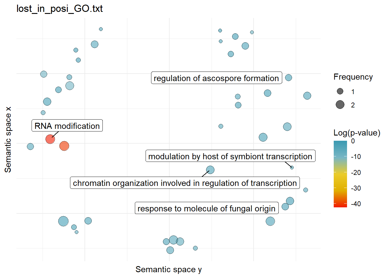
$lost_in_zmar_GO.txtWarning: ggrepel: 43 unlabeled data points (too many overlaps). Consider
increasing max.overlaps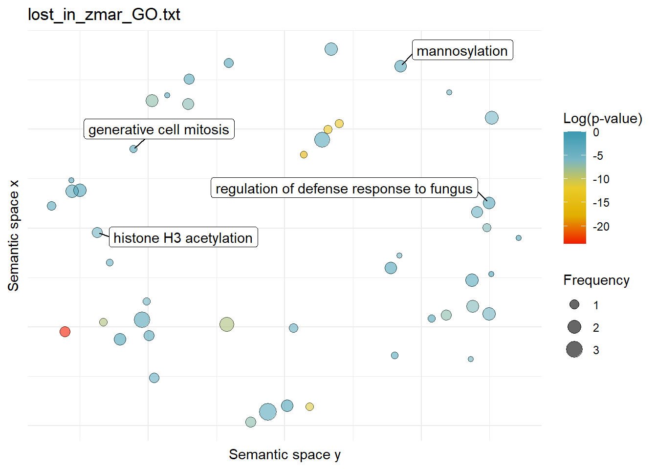
$lost_in_zmuel_GO.txtWarning: ggrepel: 1 unlabeled data points (too many overlaps). Consider
increasing max.overlaps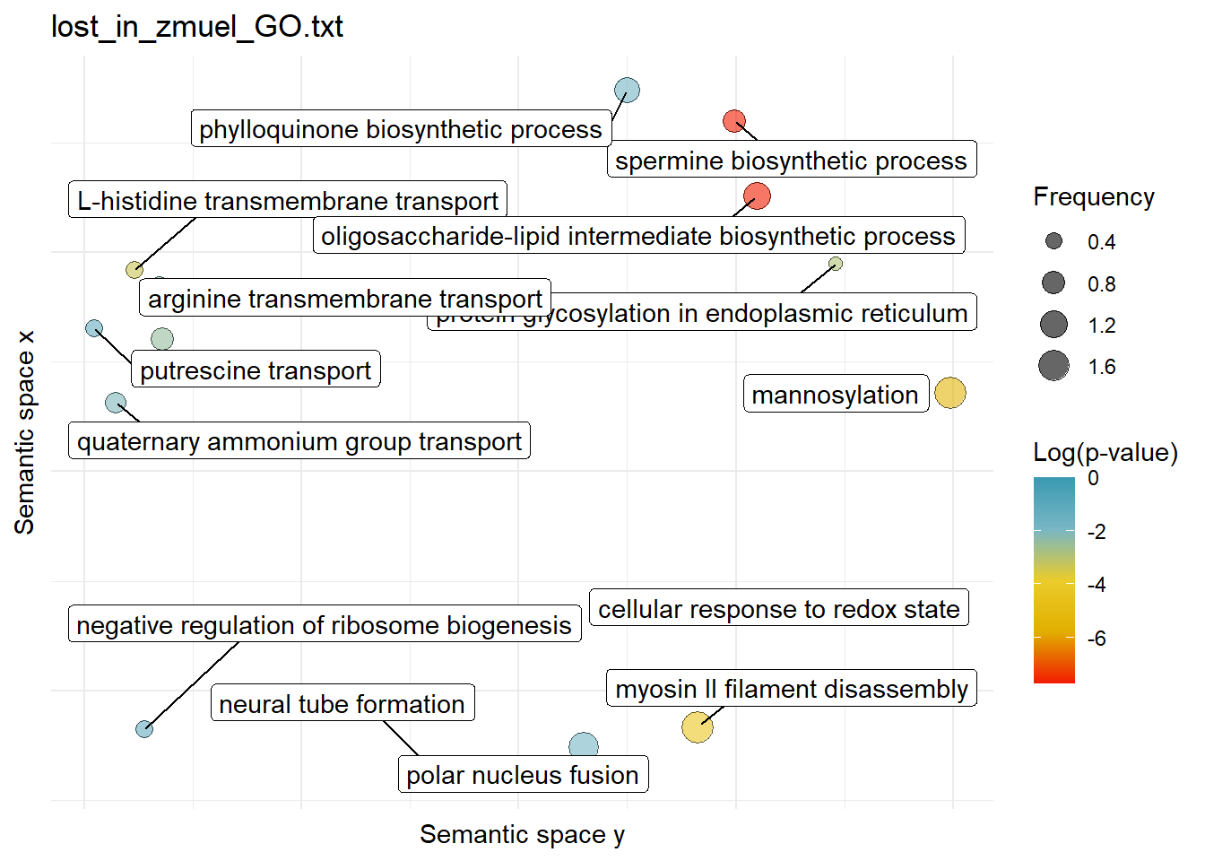
$missing_amphi_vs_all_GO.txtWarning: ggrepel: 244 unlabeled data points (too many overlaps). Consider
increasing max.overlaps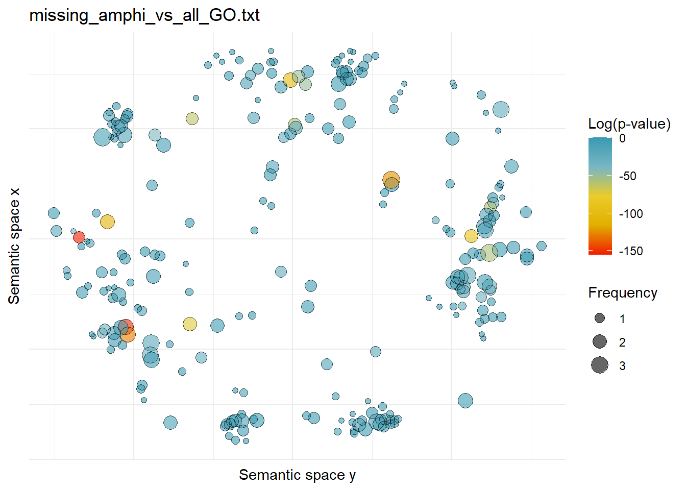
$missing_aquatics_GO.txtWarning: ggrepel: 145 unlabeled data points (too many overlaps). Consider
increasing max.overlaps
$missing_arabidopsis_vs_all_GO.txtWarning: ggrepel: 119 unlabeled data points (too many overlaps). Consider
increasing max.overlaps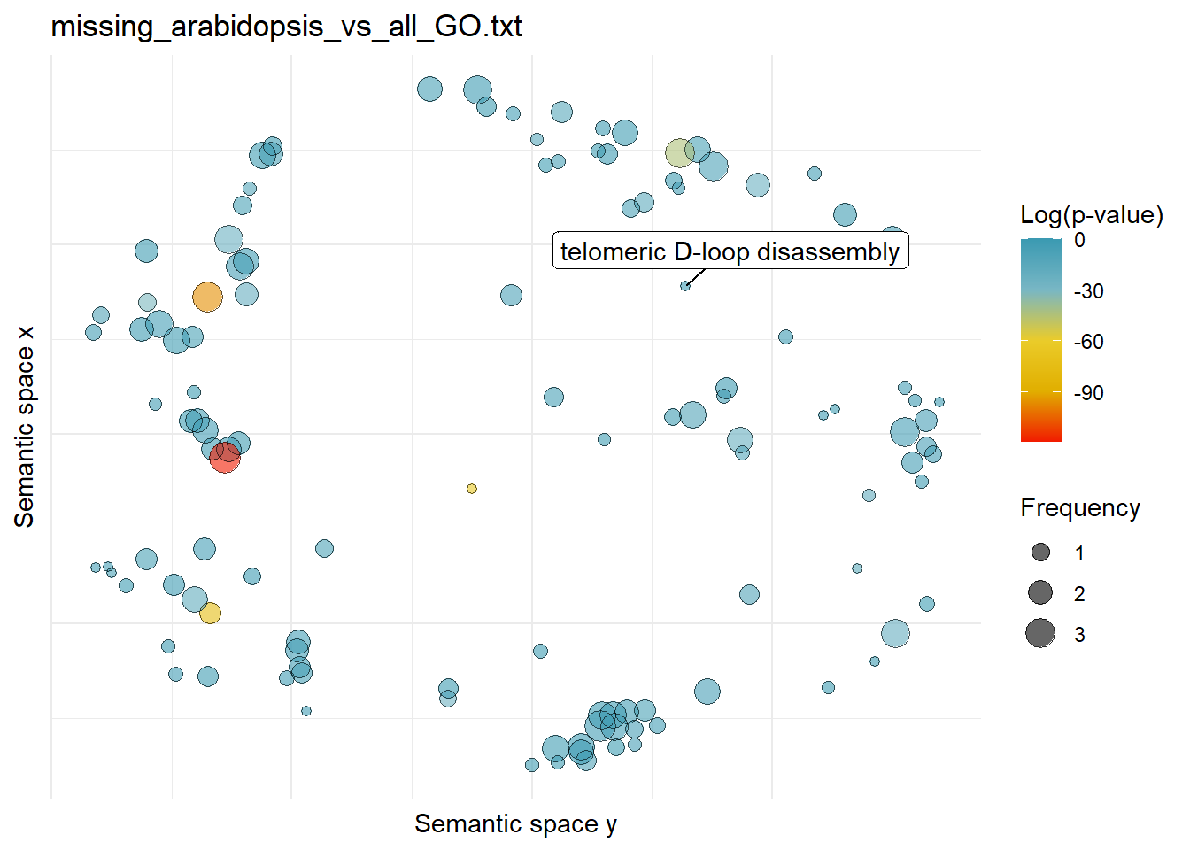
$missing_posi_vs_all_GO.txtWarning: ggrepel: 230 unlabeled data points (too many overlaps). Consider
increasing max.overlaps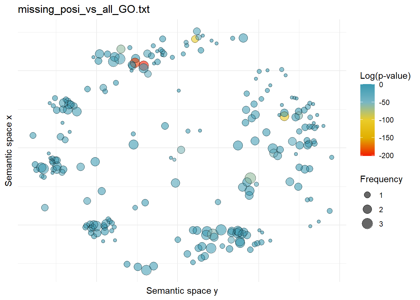
$missing_seagrasses_GO.txtWarning: ggrepel: 166 unlabeled data points (too many overlaps). Consider
increasing max.overlaps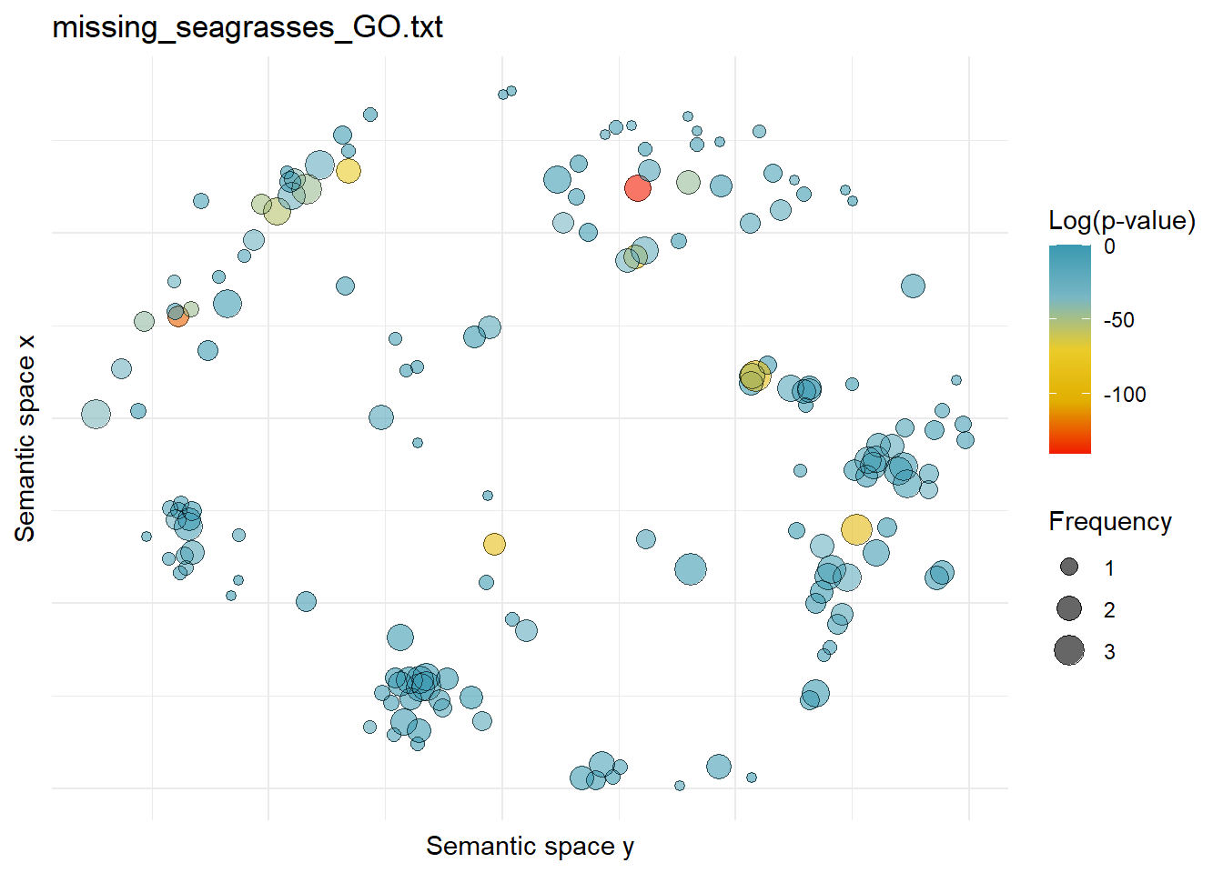
$missing_zmar_vs_all_GO.txtWarning: ggrepel: 220 unlabeled data points (too many overlaps). Consider
increasing max.overlaps
$missing_zmuel_vs_all_GO.txtWarning: ggrepel: 219 unlabeled data points (too many overlaps). Consider
increasing max.overlaps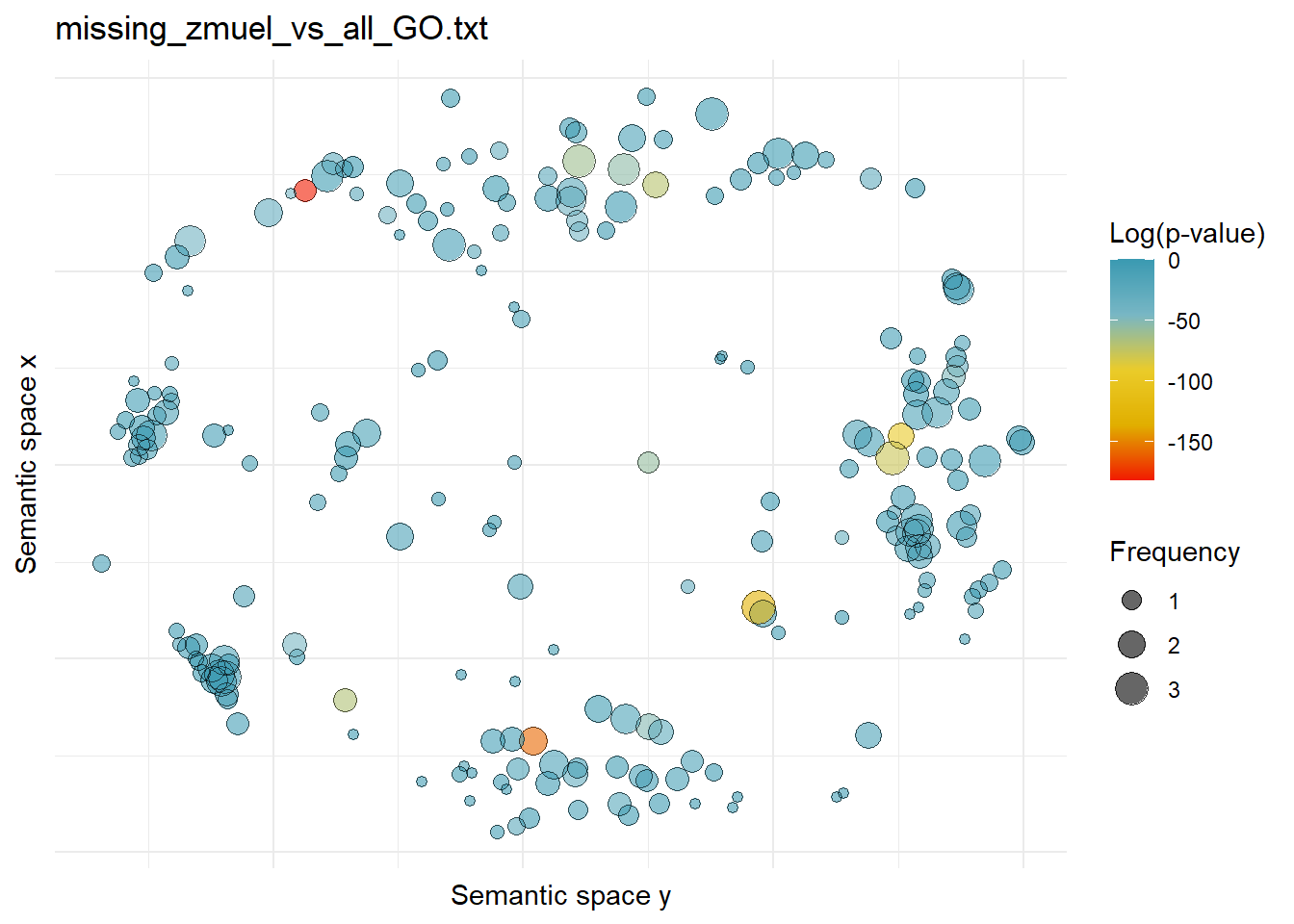
$only_in_posi_GO.txt
$only_in_zmar_GO.txtWarning: ggrepel: 5 unlabeled data points (too many overlaps). Consider
increasing max.overlaps
$only_in_zmuel_GO.txtWarning: ggrepel: 5 unlabeled data points (too many overlaps). Consider
increasing max.overlaps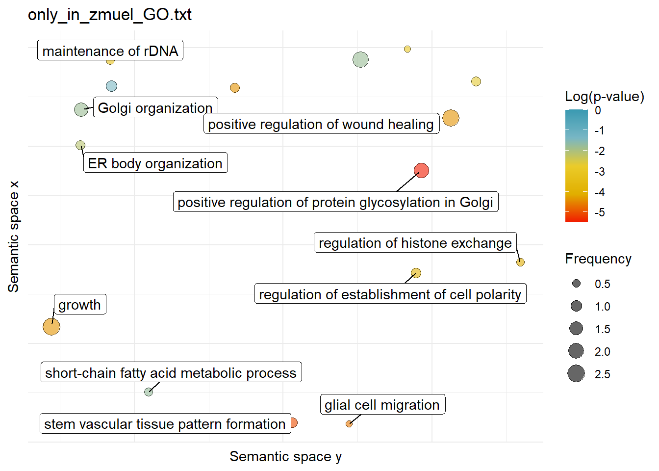
$only_seagrasses_GO.txtWarning: ggrepel: 29 unlabeled data points (too many overlaps). Consider
increasing max.overlaps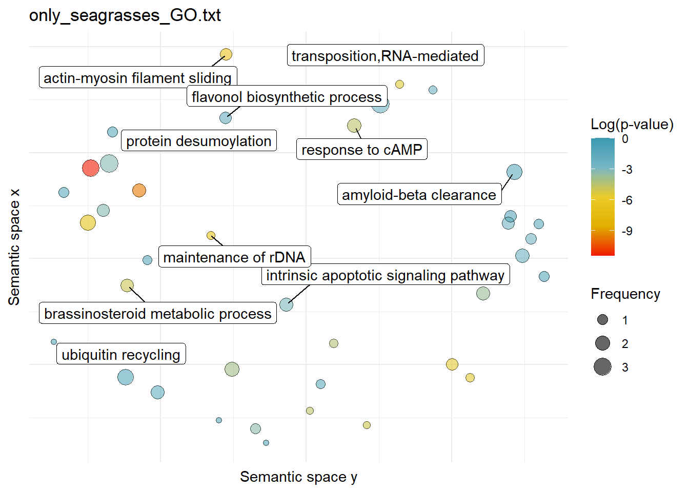
How many shared lost GO-terms are there? Hopefully, all four species will have lost the most GO-terms.
a <- list(`P. australis` = results_list$missing_posi_vs_all_GO.txt$Name,
          `A. antarctica` = results_list$missing_amphi_vs_all_GO.txt$Name,
          `Z. marina` = results_list$missing_zmar_vs_all_GO.txt$Name,
          `Z. muelleri` = results_list$missing_zmuel_vs_all_GO.txt$Name,
          `A. thaliana` = results_list$missing_arabidopsis_vs_all_GO.txt$Name)

a_go_ids <- list(`P. australis` = results_list$missing_posi_vs_all_GO.txt$TermID,
          `A. antarctica` = results_list$missing_amphi_vs_all_GO.txt$TermID,
          `Z. marina` = results_list$missing_zmar_vs_all_GO.txt$TermID,
          `Z. muelleri` = results_list$missing_zmuel_vs_all_GO.txt$TermID,
          `A. thaliana` = results_list$missing_arabidopsis_vs_all_GO.txt$TermID)
plot(euler(a),
quantities = TRUE,
fill = rev(wes_palette("Zissou1", 15, type = 'continuous')),
alpha = 0.5,
labels = list(font = 4))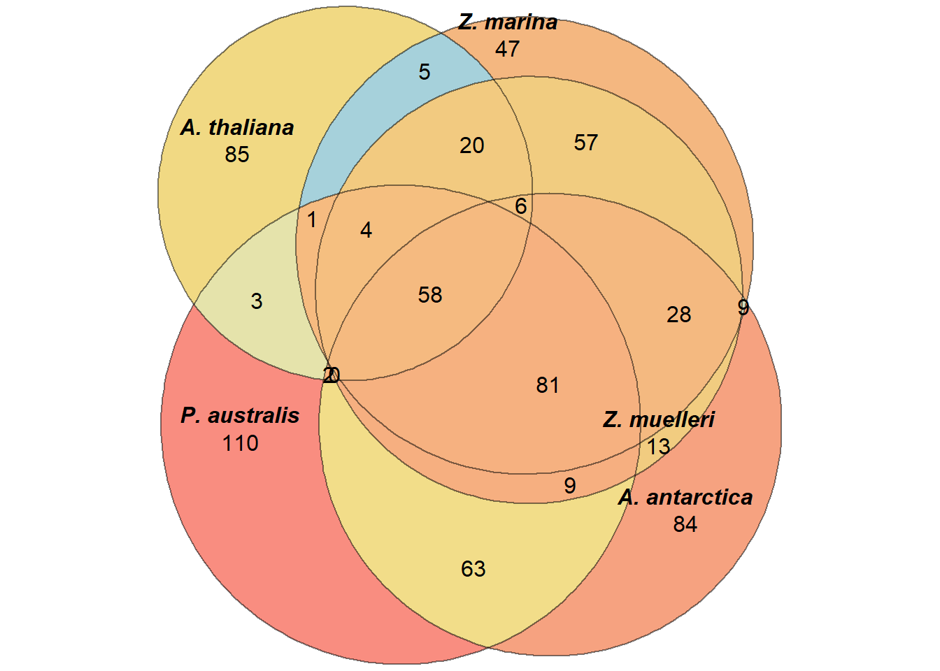
upset(fromList(a), order.by='freq', )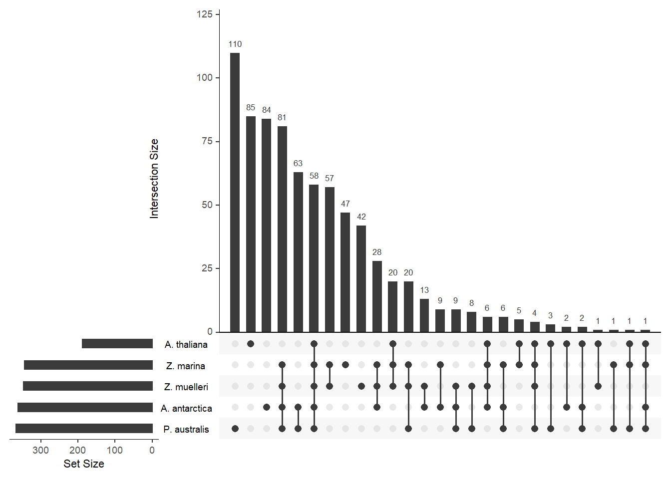
a_no_ara <- list(`P. australis` = results_list$missing_posi_vs_all_GO.txt$Name,
          `A. antarctica` = results_list$missing_amphi_vs_all_GO.txt$Name,
          `Z. marina` = results_list$missing_zmar_vs_all_GO.txt$Name,
          `Z. muelleri` = results_list$missing_zmuel_vs_all_GO.txt$Name)
What are the shared GO-terms in seagrasses, WITHOUT the Ara loss??
setdiff(Reduce(intersect, a_no_ara), Reduce(intersect, a)) %>% enframe() %>% writexl::write_xlsx('./data/shared_lost_genes.xlsx')What if we remove Posidonia?
b <- list(`A. antarctica` = results_list$missing_amphi_vs_all_GO.txt$Name,
          `Z. marina` = results_list$missing_zmar_vs_all_GO.txt$Name,
          `Z. muelleri` = results_list$missing_zmuel_vs_all_GO.txt$Name)
intersections <- Reduce(intersect, b)
intersections[grepl('ethylene', intersections)]
[1] "jasmonic acid and ethylene-dependent systemic resistance,ethylene mediated signaling pathway"
[2] "regulation of ethylene-activated signaling pathway" OK we need a big list of all GO-terms here - which GO-term is lost in which species. That will be a supplementary table.
all_species <- c("P. australis","A. antarctica","Z. marina","Z. muelleri", 'A. thaliana')
all_go_terms <- Reduce(union, a)
all_go_ids <- Reduce(union, a_go_ids)
results_d <- data.frame('GOID' = character(),
                        'GO' = character(),
                        'P. australis' = character(),
                        'A. antarctica' = character(),
                        'Z. marina' = character(),
                        'Z. muelleri' = character(),
                        'A. thaliana' = character())


for (index in seq_along(all_go_terms)){
  go <- all_go_terms[index]
  go_id <- all_go_ids[index]
  specs <- c()
  for (species in names(a)) {
    if ( length(a[[species]][grep(paste('^', go, '$', sep=''), a[[species]])]) > 0 ) {
      specs <- c(specs, species)
    }
  }

  results_d[index,] <- c(go_id, go, gsub('FALSE', 'Present', gsub('TRUE', 'Lost', all_species %in% specs)))
}
writexl::write_xlsx(results_d, 'data/Lost_GO_terms_in_five_species.xlsx')after filtering for plant-specific GO-terms
We will use the GO-terms that are plant-specific as identified by the GOMAP paper. See https://github.com/wkpalan/GOMAP-maize-analysis/blob/main/6.plantSpecific/1.getSppSpecific.R or https://plantmethods.biomedcentral.com/articles/10.1186/s13007-021-00754-1
go_plant <- read_tsv('https://raw.githubusercontent.com/wkpalan/GOMAP-maize-analysis/main/data/go/speciesSpecificGOTerms.txt')Rows: 45031 Columns: 5-- Column specification --------------------------------------------------------
Delimiter: "\t"
chr (1): GOterm
dbl (4): NCBITaxon:10090, NCBITaxon:33090, NCBITaxon:3702, NCBITaxon:40674
i Use `spec()` to retrieve the full column specification for this data.
i Specify the column types or set `show_col_types = FALSE` to quiet this message.
# taxon 33090 is Viridiplantae
plantSpecificGO <- go_plant %>% dplyr::filter(`NCBITaxon:33090`==1) %>% pull(GOterm)
plantSpecificGO <- c(plantSpecificGO,c("GO:0005575","GO:0008150","GO:0003674"))results_d %>% filter(GOID %in% plantSpecificGO) %>% writexl::write_xlsx('data/Lost_GO_terms_in_five_species.PlantSpecific.xlsx')Now let’s redo the Venn diagram with those filtered GO-terms
filters <- lapply(a_go_ids, function(ch) ch %in% plantSpecificGO)

newa <- list()
for (species in names(filters)) {
  before <- a[[species]]
  after <- before[filters[[species]]]
  newa[[species]] <- after
}
plot(euler(newa),
quantities = TRUE,
fill = rev(wes_palette("Zissou1", 15, type = 'continuous')),
alpha = 0.5,
labels = list(font = 4))
Not much difference?
sessionInfo()R version 4.1.1 (2021-08-10)
Platform: x86_64-w64-mingw32/x64 (64-bit)
Running under: Windows 10 x64 (build 17134)
Matrix products: default
locale:
[1] LC_COLLATE=English_Australia.1252 LC_CTYPE=English_Australia.1252
[3] LC_MONETARY=English_Australia.1252 LC_NUMERIC=C
[5] LC_TIME=English_Australia.1252
attached base packages:
[1] stats4 parallel stats graphics grDevices utils datasets
[8] methods base
other attached packages:
[1] rrvgo_1.4.4 UpSetR_1.4.0 eulerr_6.1.1
[4] ggrepel_0.9.1 stringi_1.7.5 httr_1.4.2
[7] wesanderson_0.3.6 rvest_1.0.1 forcats_0.5.1
[10] stringr_1.4.0 dplyr_1.0.7 purrr_0.3.4
[13] readr_2.0.2 tidyr_1.1.4 tibble_3.1.5
[16] ggplot2_3.3.5 tidyverse_1.3.1 topGO_2.44.0
[19] SparseM_1.81 GO.db_3.13.0 AnnotationDbi_1.54.1
[22] IRanges_2.26.0 S4Vectors_0.30.2 Biobase_2.52.0
[25] graph_1.70.0 BiocGenerics_0.38.0 workflowr_1.6.2
loaded via a namespace (and not attached):
[1] colorspace_2.0-2 ellipsis_0.3.2 rprojroot_2.0.2
[4] XVector_0.32.0 fs_1.5.0 rstudioapi_0.13
[7] farver_2.1.0 bit64_4.0.5 fansi_0.5.0
[10] lubridate_1.7.10 xml2_1.3.2 cachem_1.0.6
[13] GOSemSim_2.18.1 knitr_1.36 polyclip_1.10-0
[16] jsonlite_1.7.2 broom_0.7.9 gridBase_0.4-7
[19] dbplyr_2.1.1 png_0.1-7 pheatmap_1.0.12
[22] shiny_1.7.1 compiler_4.1.1 backports_1.2.1
[25] assertthat_0.2.1 fastmap_1.1.0 cli_3.0.1
[28] later_1.3.0 htmltools_0.5.2 tools_4.1.1
[31] igraph_1.2.6 NLP_0.2-1 gtable_0.3.0
[34] glue_1.4.2 GenomeInfoDbData_1.2.6 Rcpp_1.0.7
[37] slam_0.1-48 cellranger_1.1.0 jquerylib_0.1.4
[40] vctrs_0.3.8 Biostrings_2.60.2 writexl_1.4.0
[43] polylabelr_0.2.0 xfun_0.26 mime_0.12
[46] lifecycle_1.0.1 zlibbioc_1.38.0 scales_1.1.1
[49] treemap_2.4-3 vroom_1.5.5 hms_1.1.1
[52] promises_1.2.0.1 RColorBrewer_1.1-2 yaml_2.2.1
[55] curl_4.3.2 memoise_2.0.0 gridExtra_2.3
[58] sass_0.4.0 RSQLite_2.2.8 highr_0.9
[61] GenomeInfoDb_1.28.4 rlang_0.4.11 pkgconfig_2.0.3
[64] matrixStats_0.61.0 bitops_1.0-7 evaluate_0.14
[67] lattice_0.20-44 labeling_0.4.2 bit_4.0.4
[70] tidyselect_1.1.1 plyr_1.8.6 magrittr_2.0.1
[73] R6_2.5.1 generics_0.1.0 DBI_1.1.1
[76] pillar_1.6.3 haven_2.4.3 whisker_0.4
[79] withr_2.4.2 KEGGREST_1.32.0 RCurl_1.98-1.5
[82] modelr_0.1.8 crayon_1.4.1 wordcloud_2.6
[85] utf8_1.2.2 tzdb_0.1.2 rmarkdown_2.11
[88] grid_4.1.1 readxl_1.3.1 data.table_1.14.2
[91] blob_1.2.2 git2r_0.28.0 reprex_2.0.1
[94] digest_0.6.28 xtable_1.8-4 tm_0.7-8
[97] httpuv_1.6.3 munsell_0.5.0 bslib_0.3.1