Clustering/Orthofinder analysis
Philipp Bayer
15 April 2021
Last updated: 2021-04-15
Checks: 7 0
Knit directory: Amphibolis_Posidonia_Comparison/
This reproducible R Markdown analysis was created with workflowr (version 1.6.2.9000). The Checks tab describes the reproducibility checks that were applied when the results were created. The Past versions tab lists the development history.
Great! Since the R Markdown file has been committed to the Git repository, you know the exact version of the code that produced these results.
Great job! The global environment was empty. Objects defined in the global environment can affect the analysis in your R Markdown file in unknown ways. For reproduciblity it’s best to always run the code in an empty environment.
The command set.seed(20210414) was run prior to running the code in the R Markdown file. Setting a seed ensures that any results that rely on randomness, e.g. subsampling or permutations, are reproducible.
Great job! Recording the operating system, R version, and package versions is critical for reproducibility.
Nice! There were no cached chunks for this analysis, so you can be confident that you successfully produced the results during this run.
Great job! Using relative paths to the files within your workflowr project makes it easier to run your code on other machines.
Great! You are using Git for version control. Tracking code development and connecting the code version to the results is critical for reproducibility.
The results in this page were generated with repository version 49dcbb8. See the Past versions tab to see a history of the changes made to the R Markdown and HTML files.
Note that you need to be careful to ensure that all relevant files for the analysis have been committed to Git prior to generating the results (you can use wflow_publish or wflow_git_commit). workflowr only checks the R Markdown file, but you know if there are other scripts or data files that it depends on. Below is the status of the Git repository when the results were generated:
Ignored files:
    Ignored:    .Rhistory
    Ignored:    .Rproj.user/
    Ignored:    analysis/OTT.nb.html

Untracked files:
    Untracked:  species.csv
Note that any generated files, e.g. HTML, png, CSS, etc., are not included in this status report because it is ok for generated content to have uncommitted changes.
These are the previous versions of the repository in which changes were made to the R Markdown (analysis/Orthofinder.Rmd) and HTML (docs/Orthofinder.html) files. If you’ve configured a remote Git repository (see ?wflow_git_remote), click on the hyperlinks in the table below to view the files as they were in that past version.
| File | Version | Author | Date | Message |
|---|---|---|---|---|
| Rmd | 49dcbb8 | Philipp Bayer | 2021-04-15 | wflow_publish(files = list.files(“analysis/”, pattern = "*Rmd", |
library(tidyverse)-- Attaching packages ------------------------------------------------------------------------------------------------------------------- tidyverse 1.3.0 --v ggplot2 3.3.2 v purrr 0.3.4
v tibble 3.0.2 v dplyr 1.0.0
v tidyr 1.1.0 v stringr 1.4.0
v readr 1.3.1 v forcats 0.5.0-- Conflicts ---------------------------------------------------------------------------------------------------------------------- tidyverse_conflicts() --
x dplyr::filter() masks stats::filter()
x dplyr::lag() masks stats::lag()library(cowplot)
********************************************************Note: As of version 1.0.0, cowplot does not change the default ggplot2 theme anymore. To recover the previous behavior, execute:
theme_set(theme_cowplot())********************************************************theme_set(theme_cowplot())
library(RColorBrewer)
library(patchwork)
Attaching package: 'patchwork'The following object is masked from 'package:cowplot':
align_plotslibrary(UpSetR)groups <- read_tsv('data/Orthogroups.tsv') Parsed with column specification:
cols(
Orthogroup = col_character(),
Amphibolis_final.genome.scf.bigger1kbp.all.maker.proteins = col_character(),
Atrichopoda_291_v1.0.protein_primaryTranscriptOnly = col_character(),
Bdistachyon_556_v3.2.protein_primaryTranscriptOnly = col_character(),
Creinhardtii_281_v5.6.protein_primaryTranscriptOnly = col_character(),
Lemna_gibba.prots = col_character(),
Osativa_323_v7.0.protein_primaryTranscriptOnly = col_character(),
P_australis_genome_bigger1kbp.all.maker.proteins = col_character(),
Ppatens_318_v3.3.protein_primaryTranscriptOnly = col_character(),
Ptrichocarpa_533_v4.1.protein_primaryTranscriptOnly = col_character(),
Smoellendorffii_91_v1.0.protein_primaryTranscriptOnly = col_character(),
Sp9509_oxford_v3.proteins = col_character(),
TAIR10_pep_20101214 = col_character(),
TpV84ORFs.protein = col_character(),
Vvinifera_457_v2.1.protein_primaryTranscriptOnly = col_character(),
Zmays_493_RefGen_V4.protein_primaryTranscriptOnly = col_character(),
Zmu_v1_protein = col_character(),
ZosmaV2_prot_LATEST = col_character(),
mRNA_ostlu_active_pep_20170531 = col_character()
)names(groups) <- c('Orthogroup', 'A. antarctica', 'A. trichopada', 'B. distachyon', 'C. reinhardtii', 'L. gibba', 'O. sativa', 'P. australis', 'P. patens', 'P. trichocarpa', 'S. moellendorffii', 'S. polyrhiza', 'A. thaliana', 'T. parvula', 'V. vinifera', 'Z. mays', 'Z. muelleri', 'Z. marina', 'O. lucimarinus')# for upsetr, we need to know only which OG-groups are shared between species, the actual genes don't matter
per_spec <- groups %>% pivot_longer(-Orthogroup) %>%
filter(!is.na(value)) %>% # species not in an orthogroup are still listed, they just have NA genes for this group
select(-value) # don't need all gene names, speed things up# now I want the data in this format:
# listInput <- list(one = c(1, 2, 3, 5, 7, 8, 11, 12, 13), two = c(1, 2, 4, 5,
# 10), three = c(1, 5, 6, 7, 8, 9, 10, 12, 13))
x <- per_spec %>%
select(name, Orthogroup) %>% # turn the table around
deframe() # convert to named vectormylist <- lapply(split(x, names(x)), unname) # yuck - ugly code to convert the named vector to a listx <- upset(fromList(mylist), order.by='freq', nsets = length(groups) - 1)x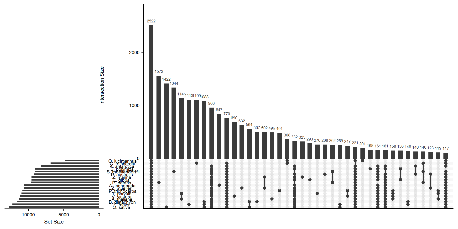
Let’s get the species-only cluster numbers
species_specific_orthos <- per_spec %>%
  group_by(Orthogroup) %>%
  summarise(counts = length(name)) %>%
  filter(counts == 1)
`summarise()` ungrouping output (override with `.groups` argument)per_spec %>%
filter(Orthogroup %in% species_specific_orthos$Orthogroup) %>%
group_by(name) %>%
count() %>%
arrange(n) %>%
knitr::kable()| name | n |
|---|---|
| A. antarctica | 74 |
| S. polyrhiza | 168 |
| O. lucimarinus | 201 |
| P. australis | 268 |
| T. parvula | 270 |
| L. gibba | 293 |
| Z. marina | 325 |
| P. trichocarpa | 491 |
| A. thaliana | 496 |
| B. distachyon | 507 |
| Z. muelleri | 632 |
| V. vinifera | 690 |
| A. trichopada | 847 |
| C. reinhardtii | 1109 |
| Z. mays | 1113 |
| S. moellendorffii | 1344 |
| O. sativa | 1422 |
| P. patens | 1572 |
species_names <- per_spec %>%
  group_by(Orthogroup) %>%
  group_by(Orthogroup) %>%
  summarise(catty = paste0(sort(name), collapse = ', '))
`summarise()` ungrouping output (override with `.groups` argument)How many orthogroups are shared between the four seagrasses?
species_names %>% dplyr::filter(catty == 'A. antarctica, P. australis, Z. marina, Z. muelleri') %>% nrow()[1] 31species_names %>% dplyr::filter(catty == 'A. antarctica, P. australis') %>% nrow()[1] 140species_names %>% dplyr::filter(catty == 'A. antarctica, P. australis, Z. marina') %>% nrow()[1] 5species_names %>% dplyr::filter(catty == 'A. antarctica, P. australis, Z. muelleri') %>% nrow()[1] 53species_names %>% dplyr::filter(catty == 'P. australis, Z. marina, Z. muelleri') %>% nrow()[1] 32I should automate this…. and I can!
newlist <- mylist[c('A. antarctica', 'Z. marina', 'P. australis', 'Z. muelleri')]

x <- upset(fromList(newlist), order.by='freq', nsets = 4)
x
This can’t be right, how are 6532 clusters suddenly shared…. that’s less than the overall. Need to subset the original clusters, NOT the species.
sessionInfo()R version 3.6.3 (2020-02-29)
Platform: x86_64-w64-mingw32/x64 (64-bit)
Running under: Windows 10 x64 (build 17134)
Matrix products: default
locale:
[1] LC_COLLATE=English_Australia.1252 LC_CTYPE=English_Australia.1252
[3] LC_MONETARY=English_Australia.1252 LC_NUMERIC=C
[5] LC_TIME=English_Australia.1252
attached base packages:
[1] stats graphics grDevices utils datasets methods base
other attached packages:
[1] UpSetR_1.4.0 patchwork_1.0.0 RColorBrewer_1.1-2
[4] cowplot_1.0.0 forcats_0.5.0 stringr_1.4.0
[7] dplyr_1.0.0 purrr_0.3.4 readr_1.3.1
[10] tidyr_1.1.0 tibble_3.0.2 ggplot2_3.3.2
[13] tidyverse_1.3.0 workflowr_1.6.2.9000
loaded via a namespace (and not attached):
[1] Rcpp_1.0.5 lubridate_1.7.9 lattice_0.20-41 getPass_0.2-2
[5] ps_1.3.4 assertthat_0.2.1 rprojroot_1.3-2 digest_0.6.25
[9] plyr_1.8.6 R6_2.4.1 cellranger_1.1.0 backports_1.1.10
[13] reprex_0.3.0 evaluate_0.14 highr_0.8 httr_1.4.2
[17] pillar_1.4.4 rlang_0.4.7 readxl_1.3.1 rstudioapi_0.11
[21] whisker_0.4 callr_3.4.4 blob_1.2.1 rmarkdown_2.3
[25] labeling_0.3 munsell_0.5.0 broom_0.5.6 compiler_3.6.3
[29] httpuv_1.5.4 modelr_0.1.8 xfun_0.17 pkgconfig_2.0.3
[33] htmltools_0.5.0 tidyselect_1.1.0 gridExtra_2.3 fansi_0.4.1
[37] crayon_1.3.4 dbplyr_1.4.4 withr_2.2.0 later_1.1.0.1
[41] grid_3.6.3 nlme_3.1-148 jsonlite_1.7.1 gtable_0.3.0
[45] lifecycle_0.2.0 DBI_1.1.0 git2r_0.27.1 magrittr_1.5
[49] scales_1.1.1 cli_2.0.2 stringi_1.5.3 farver_2.0.3
[53] fs_1.5.0.9000 promises_1.1.1 xml2_1.3.2 ellipsis_0.3.1
[57] generics_0.0.2 vctrs_0.3.1 tools_3.6.3 glue_1.4.2
[61] hms_0.5.3 processx_3.4.4 yaml_2.2.1 colorspace_1.4-1
[65] rvest_0.3.5 knitr_1.29 haven_2.3.1