first-analysis
Philipp Bayer
2020-09-17
Last updated: 2020-09-18
Checks: 7 0
Knit directory: R_gene_analysis/
This reproducible R Markdown analysis was created with workflowr (version 1.6.2). The Checks tab describes the reproducibility checks that were applied when the results were created. The Past versions tab lists the development history.
Great! Since the R Markdown file has been committed to the Git repository, you know the exact version of the code that produced these results.
Great job! The global environment was empty. Objects defined in the global environment can affect the analysis in your R Markdown file in unknown ways. For reproduciblity it’s best to always run the code in an empty environment.
The command set.seed(20200917) was run prior to running the code in the R Markdown file. Setting a seed ensures that any results that rely on randomness, e.g. subsampling or permutations, are reproducible.
Great job! Recording the operating system, R version, and package versions is critical for reproducibility.
Nice! There were no cached chunks for this analysis, so you can be confident that you successfully produced the results during this run.
Great job! Using relative paths to the files within your workflowr project makes it easier to run your code on other machines.
Great! You are using Git for version control. Tracking code development and connecting the code version to the results is critical for reproducibility.
The results in this page were generated with repository version 6f536bc. See the Past versions tab to see a history of the changes made to the R Markdown and HTML files.
Note that you need to be careful to ensure that all relevant files for the analysis have been committed to Git prior to generating the results (you can use wflow_publish or wflow_git_commit). workflowr only checks the R Markdown file, but you know if there are other scripts or data files that it depends on. Below is the status of the Git repository when the results were generated:
Ignored files:
    Ignored:    .Rhistory
    Ignored:    .Rproj.user/
Note that any generated files, e.g. HTML, png, CSS, etc., are not included in this status report because it is ok for generated content to have uncommitted changes.
These are the previous versions of the repository in which changes were made to the R Markdown (analysis/first-analysis.Rmd) and HTML (docs/first-analysis.html) files. If you’ve configured a remote Git repository (see ?wflow_git_remote), click on the hyperlinks in the table below to view the files as they were in that past version.
| File | Version | Author | Date | Message |
|---|---|---|---|---|
| Rmd | 6f536bc | Philipp Bayer | 2020-09-18 | wflow_git_commit(all = T) |
| html | 6f536bc | Philipp Bayer | 2020-09-18 | wflow_git_commit(all = T) |
library(tidyverse)-- Attaching packages ------------------------------------------------------------------------------------------------------------------ tidyverse 1.3.0 --v ggplot2 3.3.2 v purrr 0.3.4
v tibble 3.0.2 v dplyr 1.0.0
v tidyr 1.1.0 v stringr 1.4.0
v readr 1.3.1 v forcats 0.5.0-- Conflicts --------------------------------------------------------------------------------------------------------------------- tidyverse_conflicts() --
x dplyr::filter() masks stats::filter()
x dplyr::lag() masks stats::lag()library(patchwork)
library(ggsci)
library(cowplot)
********************************************************Note: As of version 1.0.0, cowplot does not change the default ggplot2 theme anymore. To recover the previous behavior, execute:
theme_set(theme_cowplot())********************************************************
Attaching package: 'cowplot'The following object is masked from 'package:patchwork':
align_plotstheme_set(theme_cowplot())Introduction
npg_col = pal_npg("nrc")(9)
col_list <- c(`Wild-type`=npg_col[8],
   Landrace = npg_col[3],
  `Old cultivar`=npg_col[2],
  `Modern cultivar`=npg_col[4])

pav_table <- read_tsv('./data/soybean_pan_pav.matrix_gene.txt')
Parsed with column specification:
cols(
.default = col_double(),
Individual = col_character()
)See spec(...) for full column specifications.pav_table# A tibble: 51,414 x 1,111
Individual `AB-01` `AB-02` `BR-01` `BR-02` `BR-03` `BR-04` `BR-05` `BR-06`
<chr> <dbl> <dbl> <dbl> <dbl> <dbl> <dbl> <dbl> <dbl>
1 GlymaLee.~ 1 1 1 1 1 1 1 1
2 GlymaLee.~ 1 1 1 1 1 1 1 1
3 GlymaLee.~ 1 1 1 1 1 1 1 1
4 GlymaLee.~ 1 1 1 1 1 1 1 1
5 GlymaLee.~ 1 1 1 1 1 1 1 1
6 GlymaLee.~ 1 1 1 1 1 1 1 1
7 GlymaLee.~ 1 1 1 1 1 1 1 1
8 GlymaLee.~ 1 1 1 1 1 1 1 1
9 GlymaLee.~ 1 1 1 1 1 1 1 1
10 GlymaLee.~ 1 1 1 1 1 1 1 1
# ... with 51,404 more rows, and 1,102 more variables: `BR-07` <dbl>,
# `BR-08` <dbl>, `BR-09` <dbl>, `BR-10` <dbl>, `BR-11` <dbl>, `BR-12` <dbl>,
# `BR-13` <dbl>, `BR-14` <dbl>, `BR-15` <dbl>, `BR-16` <dbl>, `BR-17` <dbl>,
# `BR-18` <dbl>, `BR-20` <dbl>, `BR-23` <dbl>, `BR-24` <dbl>, `BR-29` <dbl>,
# `BR-30` <dbl>, `BR-32` <dbl>, DT2000 <dbl>, ESS <dbl>, For <dbl>,
# HN001 <dbl>, HN002 <dbl>, HN003 <dbl>, HN004 <dbl>, HN005 <dbl>,
# HN006 <dbl>, HN007 <dbl>, HN008 <dbl>, HN009 <dbl>, HN010 <dbl>,
# HN011 <dbl>, HN012 <dbl>, HN013 <dbl>, HN015 <dbl>, HN016B <dbl>,
# HN017B <dbl>, HN018 <dbl>, HN019 <dbl>, HN021 <dbl>, HN022 <dbl>,
# HN023 <dbl>, HN024 <dbl>, HN025 <dbl>, HN026 <dbl>, HN027 <dbl>,
# HN028 <dbl>, HN029 <dbl>, HN030 <dbl>, HN031 <dbl>, HN032 <dbl>,
# HN033 <dbl>, HN034 <dbl>, HN035 <dbl>, HN036 <dbl>, HN037 <dbl>,
# HN038 <dbl>, HN039 <dbl>, HN040 <dbl>, HN041 <dbl>, HN042 <dbl>,
# HN043 <dbl>, HN044 <dbl>, HN045 <dbl>, HN046 <dbl>, HN047 <dbl>,
# HN048 <dbl>, HN049 <dbl>, HN050 <dbl>, HN051 <dbl>, HN052 <dbl>,
# HN053 <dbl>, HN054 <dbl>, HN055 <dbl>, HN056 <dbl>, HN057 <dbl>,
# HN058 <dbl>, HN059 <dbl>, HN060 <dbl>, HN061 <dbl>, HN062 <dbl>,
# HN063 <dbl>, HN064 <dbl>, HN065 <dbl>, HN066 <dbl>, HN067 <dbl>,
# HN068 <dbl>, HN069 <dbl>, HN070 <dbl>, HN071 <dbl>, HN072 <dbl>,
# HN073 <dbl>, HN074 <dbl>, HN075 <dbl>, HN076 <dbl>, HN077 <dbl>,
# HN078 <dbl>, HN079 <dbl>, HN080 <dbl>, HN081 <dbl>, ...NBS part
Let’s pull the NBS genes from the table
nbs <- read_tsv('./data/Lee.NBS.candidates.lst', col_names = c('Name', 'Class'))Parsed with column specification:
cols(
Name = col_character(),
Class = col_character()
)nbs# A tibble: 486 x 2
Name Class
<chr> <chr>
1 UWASoyPan00953.t1 CN
2 GlymaLee.13G222900.1.p CN
3 GlymaLee.18G227000.1.p CN
4 GlymaLee.18G080600.1.p CN
5 GlymaLee.20G036200.1.p CN
6 UWASoyPan01876.t1 CN
7 UWASoyPan04211.t1 CN
8 GlymaLee.19G105400.1.p CN
9 GlymaLee.18G085100.1.p CN
10 GlymaLee.11G142600.1.p CN
# ... with 476 more rows# have to remove the .t1s
nbs$Name <- gsub('.t1','', nbs$Name)nbs_pav_table <- pav_table %>% filter(Individual %in% nbs$Name)
nbs_pav_table# A tibble: 486 x 1,111
Individual `AB-01` `AB-02` `BR-01` `BR-02` `BR-03` `BR-04` `BR-05` `BR-06`
<chr> <dbl> <dbl> <dbl> <dbl> <dbl> <dbl> <dbl> <dbl>
1 GlymaLee.~ 1 1 1 1 1 1 1 1
2 GlymaLee.~ 1 1 1 1 1 1 1 1
3 GlymaLee.~ 1 1 1 1 1 1 1 1
4 GlymaLee.~ 1 1 1 1 1 1 1 1
5 GlymaLee.~ 1 1 1 1 1 1 1 1
6 GlymaLee.~ 1 1 1 1 1 1 1 1
7 GlymaLee.~ 1 1 1 1 1 1 1 1
8 GlymaLee.~ 1 0 1 1 1 1 1 1
9 GlymaLee.~ 1 1 1 1 1 1 1 1
10 GlymaLee.~ 1 1 1 1 1 1 1 1
# ... with 476 more rows, and 1,102 more variables: `BR-07` <dbl>,
# `BR-08` <dbl>, `BR-09` <dbl>, `BR-10` <dbl>, `BR-11` <dbl>, `BR-12` <dbl>,
# `BR-13` <dbl>, `BR-14` <dbl>, `BR-15` <dbl>, `BR-16` <dbl>, `BR-17` <dbl>,
# `BR-18` <dbl>, `BR-20` <dbl>, `BR-23` <dbl>, `BR-24` <dbl>, `BR-29` <dbl>,
# `BR-30` <dbl>, `BR-32` <dbl>, DT2000 <dbl>, ESS <dbl>, For <dbl>,
# HN001 <dbl>, HN002 <dbl>, HN003 <dbl>, HN004 <dbl>, HN005 <dbl>,
# HN006 <dbl>, HN007 <dbl>, HN008 <dbl>, HN009 <dbl>, HN010 <dbl>,
# HN011 <dbl>, HN012 <dbl>, HN013 <dbl>, HN015 <dbl>, HN016B <dbl>,
# HN017B <dbl>, HN018 <dbl>, HN019 <dbl>, HN021 <dbl>, HN022 <dbl>,
# HN023 <dbl>, HN024 <dbl>, HN025 <dbl>, HN026 <dbl>, HN027 <dbl>,
# HN028 <dbl>, HN029 <dbl>, HN030 <dbl>, HN031 <dbl>, HN032 <dbl>,
# HN033 <dbl>, HN034 <dbl>, HN035 <dbl>, HN036 <dbl>, HN037 <dbl>,
# HN038 <dbl>, HN039 <dbl>, HN040 <dbl>, HN041 <dbl>, HN042 <dbl>,
# HN043 <dbl>, HN044 <dbl>, HN045 <dbl>, HN046 <dbl>, HN047 <dbl>,
# HN048 <dbl>, HN049 <dbl>, HN050 <dbl>, HN051 <dbl>, HN052 <dbl>,
# HN053 <dbl>, HN054 <dbl>, HN055 <dbl>, HN056 <dbl>, HN057 <dbl>,
# HN058 <dbl>, HN059 <dbl>, HN060 <dbl>, HN061 <dbl>, HN062 <dbl>,
# HN063 <dbl>, HN064 <dbl>, HN065 <dbl>, HN066 <dbl>, HN067 <dbl>,
# HN068 <dbl>, HN069 <dbl>, HN070 <dbl>, HN071 <dbl>, HN072 <dbl>,
# HN073 <dbl>, HN074 <dbl>, HN075 <dbl>, HN076 <dbl>, HN077 <dbl>,
# HN078 <dbl>, HN079 <dbl>, HN080 <dbl>, HN081 <dbl>, ...names <- c()
percs <- c()
for (i in seq_along(nbs_pav_table)){
if ( i == 1) next
thisind <- colnames(nbs_pav_table)[i]
pavs <- nbs_pav_table[[i]]
perc <- sum(pavs) / length(pavs) * 100
names <- c(names, thisind)
percs <- c(percs, perc)
}
res_tibb <- new_tibble(list(names = names, percs = percs))Warning: The `nrow` argument of `new_tibble()` can't be missing as of tibble 2.0.0.
`x` must be a scalar integer.
This warning is displayed once every 8 hours.
Call `lifecycle::last_warnings()` to see where this warning was generated.res_tibb# A tibble: 1,110 x 2
names percs
<chr> <dbl>
1 AB-01 91.6
2 AB-02 93.4
3 BR-01 94.4
4 BR-02 93.0
5 BR-03 92.8
6 BR-04 93.6
7 BR-05 93.6
8 BR-06 94.0
9 BR-07 93.4
10 BR-08 93.8
# ... with 1,100 more rowsOK what do these presence percentages look like?
ggplot(data=res_tibb, aes(x=percs)) + geom_histogram(bins=25) 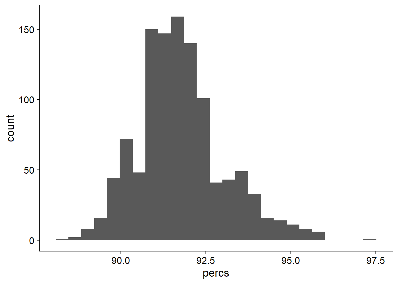
On average, 91.7701034% of NBS genes are present in each individual.
Now let’s join the table of presences to the four different types so we can group these numbers.
groups <- read_csv('./data/Table_of_cultivar_groups.csv')Parsed with column specification:
cols(
`Data-storage-ID` = col_character(),
`PI-ID` = col_character(),
`Group in violin table` = col_character()
)groups# A tibble: 1,069 x 3
`Data-storage-ID` `PI-ID` `Group in violin table`
<chr> <chr> <chr>
1 SRR1533284 PI416890 landrace
2 SRR1533282 PI323576 landrace
3 SRR1533292 PI157421 landrace
4 SRR1533216 PI594615 landrace
5 SRR1533239 PI603336 landrace
6 USB-108 PI165675 landrace
7 HNEX-13 PI253665D landrace
8 USB-382 PI603549 landrace
9 SRR1533236 PI587552 landrace
10 SRR1533332 PI567293 landrace
# ... with 1,059 more rowsjoined_groups <- left_join(res_tibb, groups, by = c('names'='Data-storage-ID'))joined_groups$`Group in violin table` <- gsub('landrace', 'Landrace', joined_groups$`Group in violin table`)
joined_groups$`Group in violin table` <- gsub('Modern_cultivar', 'Modern cultivar', joined_groups$`Group in violin table`)
joined_groups$`Group in violin table` <- gsub('Old_cultivar', 'Old cultivar', joined_groups$`Group in violin table`)
joined_groups$`Group in violin table` <- factor(joined_groups$`Group in violin table`, levels=c(NA, 'Wild-type', 'Landrace', 'Old cultivar', 'Modern cultivar'))nbs_vio <- joined_groups %>% filter(`Group in violin table` != 'NA') %>%
ggplot(aes(y=percs, x=`Group in violin table`, fill=`Group in violin table`)) +
geom_violin() +
scale_fill_manual(values=col_list)+
guides(fill = FALSE) +
ylim(c(87, 100))RLK part
Let’s do the same plot with RLKs
rlk <- read_tsv('./data/Lee.RLK.candidates.lst', col_names = c('Name', 'Class', 'Subtype'))Parsed with column specification:
cols(
Name = col_character(),
Class = col_character(),
Subtype = col_character()
)rlk# A tibble: 1,173 x 3
Name Class Subtype
<chr> <chr> <chr>
1 GlymaLee.01G001800.1.p RLK lrr
2 GlymaLee.01G004900.1.p RLK lrr
3 GlymaLee.01G007300.1.p RLK lrr
4 GlymaLee.01G007400.1.p RLK lrr
5 GlymaLee.01G012800.1.p RLK other_receptor
6 GlymaLee.01G018800.1.p RLK lrr
7 GlymaLee.01G021100.1.p RLK other_receptor
8 GlymaLee.01G025500.1.p RLK lysm
9 GlymaLee.01G026500.1.p RLK other_receptor
10 GlymaLee.01G027000.1.p RLK lrr
# ... with 1,163 more rows# have to remove the .t1s
rlk$Name <- gsub('.t1','', rlk$Name)rlk_pav_table <- pav_table %>% filter(Individual %in% rlk$Name)
rlk_pav_table# A tibble: 1,173 x 1,111
Individual `AB-01` `AB-02` `BR-01` `BR-02` `BR-03` `BR-04` `BR-05` `BR-06`
<chr> <dbl> <dbl> <dbl> <dbl> <dbl> <dbl> <dbl> <dbl>
1 GlymaLee.~ 1 1 1 1 1 1 1 1
2 GlymaLee.~ 1 1 1 1 1 1 1 1
3 GlymaLee.~ 1 1 1 1 1 1 1 1
4 GlymaLee.~ 1 1 1 1 1 1 1 1
5 GlymaLee.~ 1 1 1 1 1 1 1 1
6 GlymaLee.~ 1 1 1 1 1 1 1 1
7 GlymaLee.~ 1 1 1 1 1 1 1 1
8 GlymaLee.~ 1 1 1 1 1 1 1 1
9 GlymaLee.~ 1 1 1 1 1 1 1 1
10 GlymaLee.~ 1 1 1 1 1 1 1 1
# ... with 1,163 more rows, and 1,102 more variables: `BR-07` <dbl>,
# `BR-08` <dbl>, `BR-09` <dbl>, `BR-10` <dbl>, `BR-11` <dbl>, `BR-12` <dbl>,
# `BR-13` <dbl>, `BR-14` <dbl>, `BR-15` <dbl>, `BR-16` <dbl>, `BR-17` <dbl>,
# `BR-18` <dbl>, `BR-20` <dbl>, `BR-23` <dbl>, `BR-24` <dbl>, `BR-29` <dbl>,
# `BR-30` <dbl>, `BR-32` <dbl>, DT2000 <dbl>, ESS <dbl>, For <dbl>,
# HN001 <dbl>, HN002 <dbl>, HN003 <dbl>, HN004 <dbl>, HN005 <dbl>,
# HN006 <dbl>, HN007 <dbl>, HN008 <dbl>, HN009 <dbl>, HN010 <dbl>,
# HN011 <dbl>, HN012 <dbl>, HN013 <dbl>, HN015 <dbl>, HN016B <dbl>,
# HN017B <dbl>, HN018 <dbl>, HN019 <dbl>, HN021 <dbl>, HN022 <dbl>,
# HN023 <dbl>, HN024 <dbl>, HN025 <dbl>, HN026 <dbl>, HN027 <dbl>,
# HN028 <dbl>, HN029 <dbl>, HN030 <dbl>, HN031 <dbl>, HN032 <dbl>,
# HN033 <dbl>, HN034 <dbl>, HN035 <dbl>, HN036 <dbl>, HN037 <dbl>,
# HN038 <dbl>, HN039 <dbl>, HN040 <dbl>, HN041 <dbl>, HN042 <dbl>,
# HN043 <dbl>, HN044 <dbl>, HN045 <dbl>, HN046 <dbl>, HN047 <dbl>,
# HN048 <dbl>, HN049 <dbl>, HN050 <dbl>, HN051 <dbl>, HN052 <dbl>,
# HN053 <dbl>, HN054 <dbl>, HN055 <dbl>, HN056 <dbl>, HN057 <dbl>,
# HN058 <dbl>, HN059 <dbl>, HN060 <dbl>, HN061 <dbl>, HN062 <dbl>,
# HN063 <dbl>, HN064 <dbl>, HN065 <dbl>, HN066 <dbl>, HN067 <dbl>,
# HN068 <dbl>, HN069 <dbl>, HN070 <dbl>, HN071 <dbl>, HN072 <dbl>,
# HN073 <dbl>, HN074 <dbl>, HN075 <dbl>, HN076 <dbl>, HN077 <dbl>,
# HN078 <dbl>, HN079 <dbl>, HN080 <dbl>, HN081 <dbl>, ...names <- c()
percs <- c()
for (i in seq_along(rlk_pav_table)){
if ( i == 1) next
thisind <- colnames(rlk_pav_table)[i]
pavs <- rlk_pav_table[[i]]
perc <- sum(pavs) / length(pavs) * 100
names <- c(names, thisind)
percs <- c(percs, perc)
}
res_tibb <- new_tibble(list(names = names, percs = percs))
res_tibb# A tibble: 1,110 x 2
names percs
<chr> <dbl>
1 AB-01 99.5
2 AB-02 99.1
3 BR-01 99.4
4 BR-02 99.3
5 BR-03 99.4
6 BR-04 99.5
7 BR-05 99.2
8 BR-06 99.5
9 BR-07 99.3
10 BR-08 99.5
# ... with 1,100 more rowsOK what do these presence percentages look like?
ggplot(data=res_tibb, aes(x=percs)) + geom_histogram(bins=25) 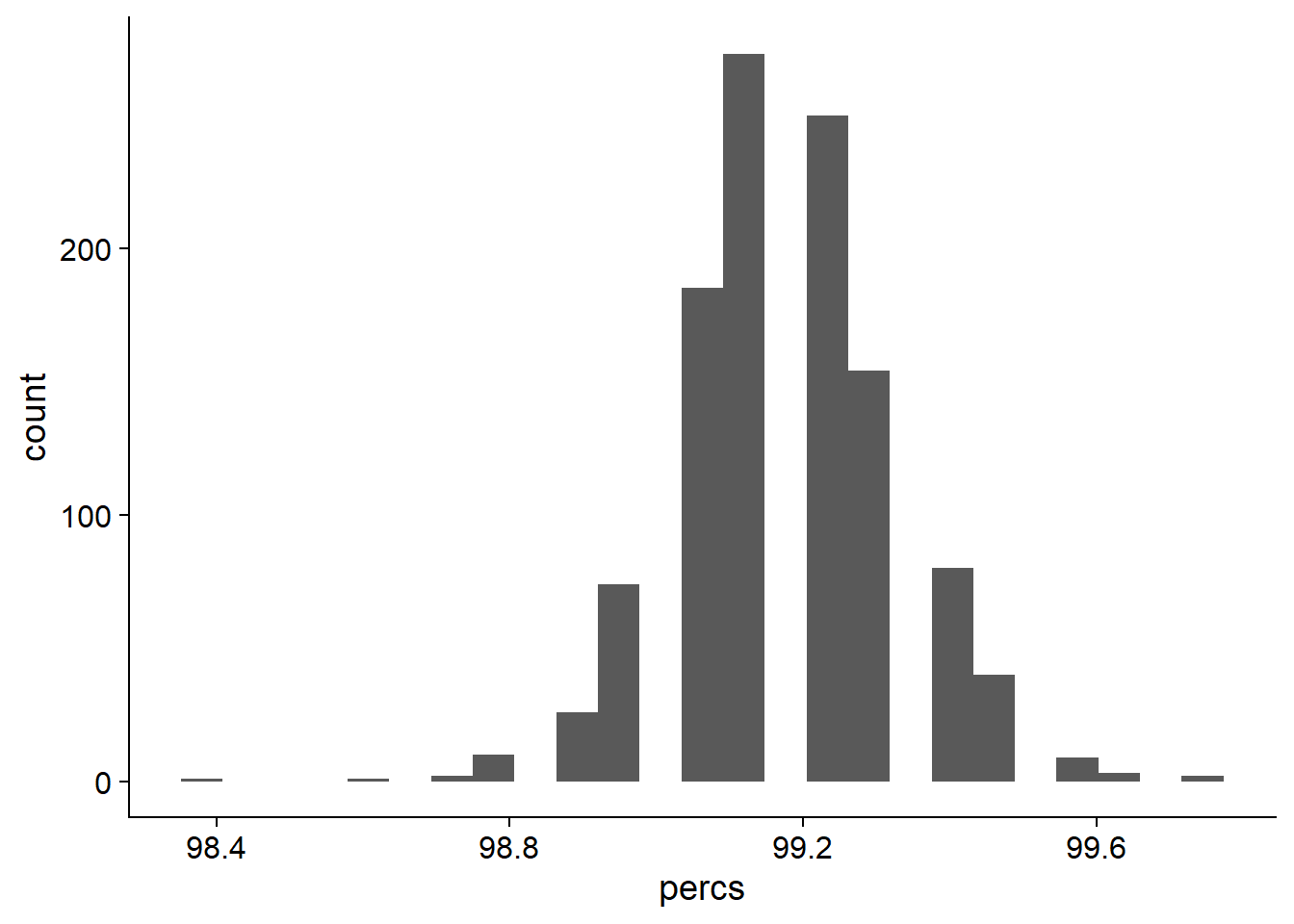
On average, 99.190418% of NBS genes are present in each individual.
Now let’s join the table of presences to the four different types so we can group these numbers.
groups <- read_csv('./data/Table_of_cultivar_groups.csv')Parsed with column specification:
cols(
`Data-storage-ID` = col_character(),
`PI-ID` = col_character(),
`Group in violin table` = col_character()
)groups# A tibble: 1,069 x 3
`Data-storage-ID` `PI-ID` `Group in violin table`
<chr> <chr> <chr>
1 SRR1533284 PI416890 landrace
2 SRR1533282 PI323576 landrace
3 SRR1533292 PI157421 landrace
4 SRR1533216 PI594615 landrace
5 SRR1533239 PI603336 landrace
6 USB-108 PI165675 landrace
7 HNEX-13 PI253665D landrace
8 USB-382 PI603549 landrace
9 SRR1533236 PI587552 landrace
10 SRR1533332 PI567293 landrace
# ... with 1,059 more rowsjoined_groups <- left_join(res_tibb, groups, by = c('names'='Data-storage-ID'))joined_groups$`Group in violin table` <- gsub('landrace', 'Landrace', joined_groups$`Group in violin table`)
joined_groups$`Group in violin table` <- gsub('Modern_cultivar', 'Modern cultivar', joined_groups$`Group in violin table`)
joined_groups$`Group in violin table` <- gsub('Old_cultivar', 'Old cultivar', joined_groups$`Group in violin table`)
joined_groups$`Group in violin table` <- factor(joined_groups$`Group in violin table`, levels=c(NA, 'Wild-type', 'Landrace', 'Old cultivar', 'Modern cultivar'))rlk_vio <- joined_groups %>% filter(`Group in violin table` != 'NA') %>%
ggplot(aes(y=percs, x=`Group in violin table`, fill=`Group in violin table`)) +
geom_violin() +
scale_fill_manual(values=col_list) +
guides(fill = FALSE) +
ylim(c(87, 100))RLP part
And now with RLPs
rlp <- read_tsv('./data/Lee.RLP.candidates.lst', col_names = c('Name', 'Class', 'Subtype'))Parsed with column specification:
cols(
Name = col_character(),
Class = col_character(),
Subtype = col_character()
)rlp# A tibble: 180 x 3
Name Class Subtype
<chr> <chr> <chr>
1 GlymaLee.01G033200.1.p RLP lrr
2 GlymaLee.01G071200.1.p RLP lrr
3 GlymaLee.01G073300.1.p RLP lrr
4 GlymaLee.01G091600.1.p RLP lrr
5 GlymaLee.01G091700.1.p RLP lrr
6 GlymaLee.01G093500.1.p RLP lrr
7 GlymaLee.01G099100.1.p RLP lrr
8 GlymaLee.01G100300.1.p RLP lrr
9 GlymaLee.01G118800.1.p RLP lrr
10 GlymaLee.01G121400.1.p RLP lrr
# ... with 170 more rows# have to remove the .t1s
rlp$Name <- gsub('.t1','', rlp$Name)rlp_pav_table <- pav_table %>% filter(Individual %in% rlp$Name)
rlp_pav_table# A tibble: 180 x 1,111
Individual `AB-01` `AB-02` `BR-01` `BR-02` `BR-03` `BR-04` `BR-05` `BR-06`
<chr> <dbl> <dbl> <dbl> <dbl> <dbl> <dbl> <dbl> <dbl>
1 GlymaLee.~ 1 1 1 1 1 1 1 1
2 GlymaLee.~ 1 1 1 1 1 1 1 1
3 GlymaLee.~ 1 1 1 1 1 1 1 1
4 GlymaLee.~ 1 1 1 1 1 1 1 1
5 GlymaLee.~ 1 1 1 1 1 1 1 1
6 GlymaLee.~ 1 1 1 1 0 1 1 1
7 GlymaLee.~ 1 1 1 1 1 1 1 1
8 GlymaLee.~ 1 1 1 1 1 1 1 1
9 GlymaLee.~ 1 1 1 1 1 1 1 1
10 GlymaLee.~ 1 1 1 1 1 1 1 1
# ... with 170 more rows, and 1,102 more variables: `BR-07` <dbl>,
# `BR-08` <dbl>, `BR-09` <dbl>, `BR-10` <dbl>, `BR-11` <dbl>, `BR-12` <dbl>,
# `BR-13` <dbl>, `BR-14` <dbl>, `BR-15` <dbl>, `BR-16` <dbl>, `BR-17` <dbl>,
# `BR-18` <dbl>, `BR-20` <dbl>, `BR-23` <dbl>, `BR-24` <dbl>, `BR-29` <dbl>,
# `BR-30` <dbl>, `BR-32` <dbl>, DT2000 <dbl>, ESS <dbl>, For <dbl>,
# HN001 <dbl>, HN002 <dbl>, HN003 <dbl>, HN004 <dbl>, HN005 <dbl>,
# HN006 <dbl>, HN007 <dbl>, HN008 <dbl>, HN009 <dbl>, HN010 <dbl>,
# HN011 <dbl>, HN012 <dbl>, HN013 <dbl>, HN015 <dbl>, HN016B <dbl>,
# HN017B <dbl>, HN018 <dbl>, HN019 <dbl>, HN021 <dbl>, HN022 <dbl>,
# HN023 <dbl>, HN024 <dbl>, HN025 <dbl>, HN026 <dbl>, HN027 <dbl>,
# HN028 <dbl>, HN029 <dbl>, HN030 <dbl>, HN031 <dbl>, HN032 <dbl>,
# HN033 <dbl>, HN034 <dbl>, HN035 <dbl>, HN036 <dbl>, HN037 <dbl>,
# HN038 <dbl>, HN039 <dbl>, HN040 <dbl>, HN041 <dbl>, HN042 <dbl>,
# HN043 <dbl>, HN044 <dbl>, HN045 <dbl>, HN046 <dbl>, HN047 <dbl>,
# HN048 <dbl>, HN049 <dbl>, HN050 <dbl>, HN051 <dbl>, HN052 <dbl>,
# HN053 <dbl>, HN054 <dbl>, HN055 <dbl>, HN056 <dbl>, HN057 <dbl>,
# HN058 <dbl>, HN059 <dbl>, HN060 <dbl>, HN061 <dbl>, HN062 <dbl>,
# HN063 <dbl>, HN064 <dbl>, HN065 <dbl>, HN066 <dbl>, HN067 <dbl>,
# HN068 <dbl>, HN069 <dbl>, HN070 <dbl>, HN071 <dbl>, HN072 <dbl>,
# HN073 <dbl>, HN074 <dbl>, HN075 <dbl>, HN076 <dbl>, HN077 <dbl>,
# HN078 <dbl>, HN079 <dbl>, HN080 <dbl>, HN081 <dbl>, ...names <- c()
percs <- c()
for (i in seq_along(rlp_pav_table)){
if ( i == 1) next
thisind <- colnames(rlp_pav_table)[i]
pavs <- rlp_pav_table[[i]]
perc <- sum(pavs) / length(pavs) * 100
names <- c(names, thisind)
percs <- c(percs, perc)
}
res_tibb <- new_tibble(list(names = names, percs = percs))
res_tibb# A tibble: 1,110 x 2
names percs
<chr> <dbl>
1 AB-01 95
2 AB-02 95.6
3 BR-01 96.7
4 BR-02 95.6
5 BR-03 96.7
6 BR-04 96.1
7 BR-05 96.1
8 BR-06 96.1
9 BR-07 96.1
10 BR-08 96.1
# ... with 1,100 more rowsOK what do these presence percentages look like?
ggplot(data=res_tibb, aes(x=percs)) + geom_histogram(bins=25) 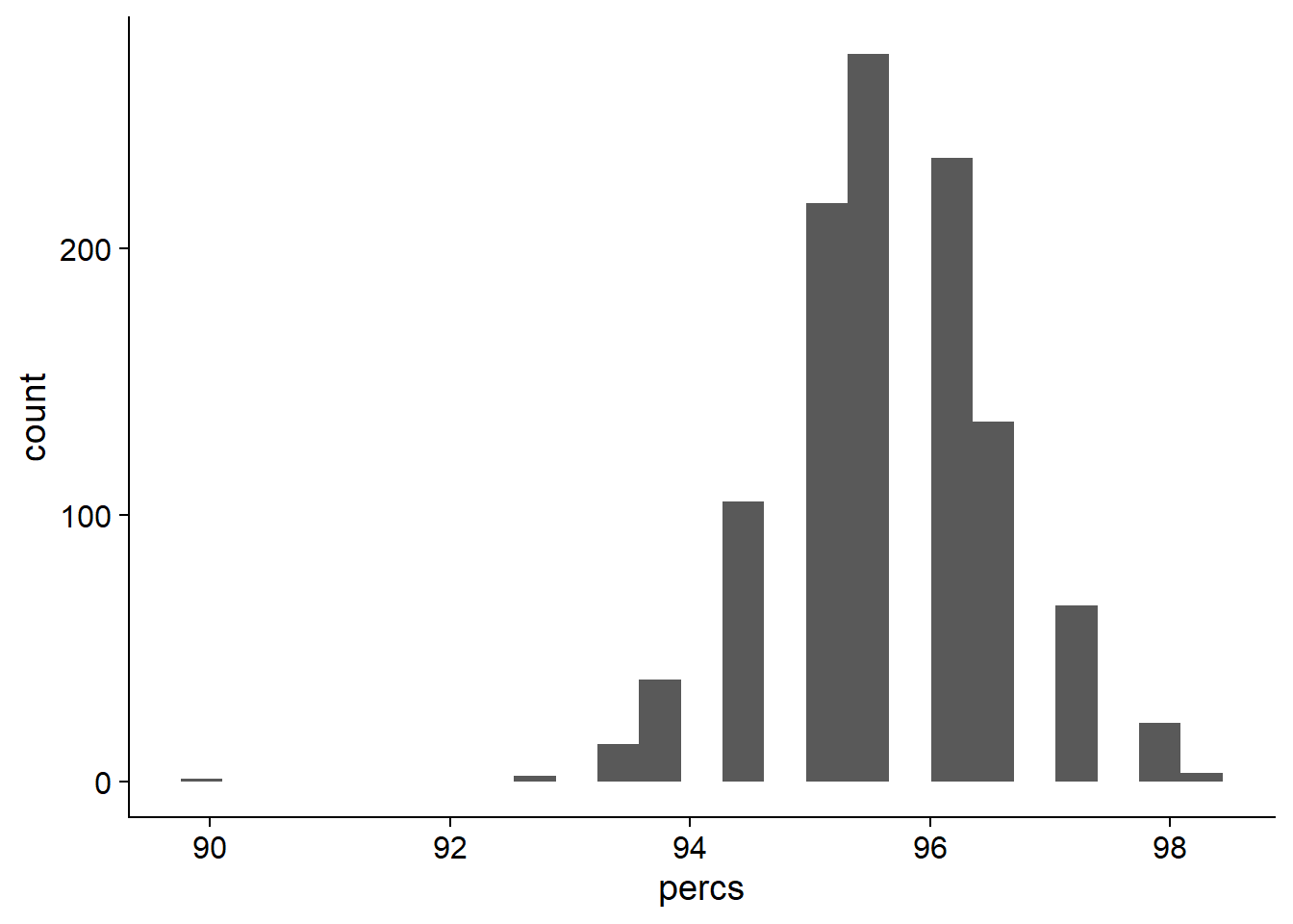
On average, 95.6496496% of NBS genes are present in each individual.
Now let’s join the table of presences to the four different types so we can group these numbers.
groups <- read_csv('./data/Table_of_cultivar_groups.csv')Parsed with column specification:
cols(
`Data-storage-ID` = col_character(),
`PI-ID` = col_character(),
`Group in violin table` = col_character()
)groups# A tibble: 1,069 x 3
`Data-storage-ID` `PI-ID` `Group in violin table`
<chr> <chr> <chr>
1 SRR1533284 PI416890 landrace
2 SRR1533282 PI323576 landrace
3 SRR1533292 PI157421 landrace
4 SRR1533216 PI594615 landrace
5 SRR1533239 PI603336 landrace
6 USB-108 PI165675 landrace
7 HNEX-13 PI253665D landrace
8 USB-382 PI603549 landrace
9 SRR1533236 PI587552 landrace
10 SRR1533332 PI567293 landrace
# ... with 1,059 more rowsjoined_groups <- left_join(res_tibb, groups, by = c('names'='Data-storage-ID'))joined_groups$`Group in violin table` <- gsub('landrace', 'Landrace', joined_groups$`Group in violin table`)
joined_groups$`Group in violin table` <- gsub('Modern_cultivar', 'Modern cultivar', joined_groups$`Group in violin table`)
joined_groups$`Group in violin table` <- gsub('Old_cultivar', 'Old cultivar', joined_groups$`Group in violin table`)
joined_groups$`Group in violin table` <- factor(joined_groups$`Group in violin table`, levels=c(NA, 'Wild-type', 'Landrace', 'Old cultivar', 'Modern cultivar'))rlp_vio <- joined_groups %>% filter(`Group in violin table` != 'NA') %>%
ggplot(aes(y=percs, x=`Group in violin table`, fill=`Group in violin table`)) +
geom_violin() +
scale_fill_manual(values=col_list) +
guides(fill = FALSE) +
ylim(c(87, 100))Plotting together
nbs_vio + rlk_vio + rlp_vio
sessionInfo()R version 3.6.3 (2020-02-29)
Platform: x86_64-w64-mingw32/x64 (64-bit)
Running under: Windows 10 x64 (build 17134)
Matrix products: default
locale:
[1] LC_COLLATE=English_Australia.1252 LC_CTYPE=English_Australia.1252
[3] LC_MONETARY=English_Australia.1252 LC_NUMERIC=C
[5] LC_TIME=English_Australia.1252
attached base packages:
[1] stats graphics grDevices utils datasets methods base
other attached packages:
[1] cowplot_1.0.0 ggsci_2.9 patchwork_1.0.0 forcats_0.5.0
[5] stringr_1.4.0 dplyr_1.0.0 purrr_0.3.4 readr_1.3.1
[9] tidyr_1.1.0 tibble_3.0.2 ggplot2_3.3.2 tidyverse_1.3.0
[13] workflowr_1.6.2
loaded via a namespace (and not attached):
[1] Rcpp_1.0.5 lubridate_1.7.9 lattice_0.20-41 assertthat_0.2.1
[5] rprojroot_1.3-2 digest_0.6.25 utf8_1.1.4 R6_2.4.1
[9] cellranger_1.1.0 backports_1.1.8 reprex_0.3.0 evaluate_0.14
[13] httr_1.4.1 pillar_1.4.4 rlang_0.4.6 readxl_1.3.1
[17] rstudioapi_0.11 whisker_0.4 blob_1.2.1 rmarkdown_2.3
[21] labeling_0.3 munsell_0.5.0 broom_0.5.6 compiler_3.6.3
[25] httpuv_1.5.4 modelr_0.1.8 xfun_0.15 pkgconfig_2.0.3
[29] htmltools_0.5.0 tidyselect_1.1.0 fansi_0.4.1 crayon_1.3.4
[33] dbplyr_1.4.4 withr_2.2.0 later_1.1.0.1 grid_3.6.3
[37] nlme_3.1-148 jsonlite_1.7.0 gtable_0.3.0 lifecycle_0.2.0
[41] DBI_1.1.0 git2r_0.26.1 magrittr_1.5 scales_1.1.1
[45] cli_2.0.2 stringi_1.4.6 farver_2.0.3 fs_1.5.0.9000
[49] promises_1.1.1 xml2_1.3.2 ellipsis_0.3.1 generics_0.0.2
[53] vctrs_0.3.1 tools_3.6.3 glue_1.4.1 hms_0.5.3
[57] yaml_2.2.1 colorspace_1.4-1 rvest_0.3.5 knitr_1.29
[61] haven_2.3.1