Linking yield with NLR PAV
Philipp Bayer
2020-09-22
Last updated: 2020-09-24
Checks: 6 1
Knit directory: R_gene_analysis/
This reproducible R Markdown analysis was created with workflowr (version 1.6.2.9000). The Checks tab describes the reproducibility checks that were applied when the results were created. The Past versions tab lists the development history.
The R Markdown is untracked by Git. To know which version of the R Markdown file created these results, you’ll want to first commit it to the Git repo. If you’re still working on the analysis, you can ignore this warning. When you’re finished, you can run wflow_publish to commit the R Markdown file and build the HTML.
Great job! The global environment was empty. Objects defined in the global environment can affect the analysis in your R Markdown file in unknown ways. For reproduciblity it’s best to always run the code in an empty environment.
The command set.seed(20200917) was run prior to running the code in the R Markdown file. Setting a seed ensures that any results that rely on randomness, e.g. subsampling or permutations, are reproducible.
Great job! Recording the operating system, R version, and package versions is critical for reproducibility.
Nice! There were no cached chunks for this analysis, so you can be confident that you successfully produced the results during this run.
Great job! Using relative paths to the files within your workflowr project makes it easier to run your code on other machines.
Great! You are using Git for version control. Tracking code development and connecting the code version to the results is critical for reproducibility.
The results in this page were generated with repository version 1b346e9. See the Past versions tab to see a history of the changes made to the R Markdown and HTML files.
Note that you need to be careful to ensure that all relevant files for the analysis have been committed to Git prior to generating the results (you can use wflow_publish or wflow_git_commit). workflowr only checks the R Markdown file, but you know if there are other scripts or data files that it depends on. Below is the status of the Git repository when the results were generated:
Ignored files:
    Ignored:    .Rhistory
    Ignored:    .Rproj.user/

Untracked files:
    Untracked:  analysis/gwas.Rmd
    Untracked:  analysis/phylo.Rmd
    Untracked:  analysis/yield_link.Rmd
    Untracked:  code/transformToGAPIT.py
    Untracked:  data/Brec_R1.txt
    Untracked:  data/Brec_R2.txt
    Untracked:  data/CR15_R1.txt
    Untracked:  data/CR15_R2.txt
    Untracked:  data/CR_14_R1.txt
    Untracked:  data/CR_14_R2.txt
    Untracked:  data/KS_R1.txt
    Untracked:  data/KS_R2.txt
    Untracked:  data/NBS_PAV.txt.gz
    Untracked:  data/NLR_PAV_GD.txt
    Untracked:  data/NLR_PAV_GM.txt
    Untracked:  data/PPR1.txt
    Untracked:  data/PPR2.txt
    Untracked:  data/bac.txt
    Untracked:  data/brown.txt
    Untracked:  data/cy3.txt
    Untracked:  data/cy5.txt
    Untracked:  data/early.txt
    Untracked:  data/flowerings.txt
    Untracked:  data/foregeye.txt
    Untracked:  data/height.txt
    Untracked:  data/late.txt
    Untracked:  data/mature.txt
    Untracked:  data/motting.txt
    Untracked:  data/oil.txt
    Untracked:  data/pdh.txt
    Untracked:  data/protein.txt
    Untracked:  data/rust_tan.txt
    Untracked:  data/salt.txt
    Untracked:  data/seedq.txt
    Untracked:  data/seedweight.txt
    Untracked:  data/stem_termination.txt
    Untracked:  data/sudden.txt
    Untracked:  data/virus.txt
    Untracked:  data/yield.txt
    Untracked:  output/GAPIT/

Unstaged changes:
    Modified:   README.md
    Modified:   analysis/index.Rmd
    Modified:   analysis/total_numbers.Rmd
Note that any generated files, e.g. HTML, png, CSS, etc., are not included in this status report because it is ok for generated content to have uncommitted changes.
There are no past versions. Publish this analysis with wflow_publish() to start tracking its development.
knitr::opts_chunk$set(warning = FALSE, message = FALSE)
library(tidyverse)
-- Attaching packages ------------------------------------------------------------------------------------------------------------------- tidyverse 1.3.0 --v ggplot2 3.3.2 v purrr 0.3.4
v tibble 3.0.2 v dplyr 1.0.0
v tidyr 1.1.0 v stringr 1.4.0
v readr 1.3.1 v forcats 0.5.0-- Conflicts ---------------------------------------------------------------------------------------------------------------------- tidyverse_conflicts() --
x dplyr::filter() masks stats::filter()
x dplyr::lag() masks stats::lag()library(patchwork)
library(ggsci)
library(dabestr)Loading required package: magrittr
Attaching package: 'magrittr'The following object is masked from 'package:purrr':
set_namesThe following object is masked from 'package:tidyr':
extractlibrary(dabestr)
library(cowplot)
********************************************************Note: As of version 1.0.0, cowplot does not change the default ggplot2 theme anymore. To recover the previous behavior, execute:
theme_set(theme_cowplot())********************************************************
Attaching package: 'cowplot'The following object is masked from 'package:patchwork':
align_plotslibrary(ggsignif)
library(ggforce)
theme_set(theme_cowplot())Data loading
npg_col = pal_npg("nrc")(9)
col_list <- c(`Wild-type`=npg_col[8],
   Landrace = npg_col[3],
  `Old cultivar`=npg_col[2],
  `Modern cultivar`=npg_col[4])

pav_table <- read_tsv('./data/soybean_pan_pav.matrix_gene.txt.gz')
nbs <- read_tsv('./data/Lee.NBS.candidates.lst', col_names = c('Name', 'Class'))
nbs# A tibble: 486 x 2
Name Class
<chr> <chr>
1 UWASoyPan00953.t1 CN
2 GlymaLee.13G222900.1.p CN
3 GlymaLee.18G227000.1.p CN
4 GlymaLee.18G080600.1.p CN
5 GlymaLee.20G036200.1.p CN
6 UWASoyPan01876.t1 CN
7 UWASoyPan04211.t1 CN
8 GlymaLee.19G105400.1.p CN
9 GlymaLee.18G085100.1.p CN
10 GlymaLee.11G142600.1.p CN
# ... with 476 more rows# have to remove the .t1s
nbs$Name <- gsub('.t1','', nbs$Name)
nbs_pav_table <- pav_table %>% filter(Individual %in% nbs$Name)names <- c()
presences <- c()
for (i in seq_along(nbs_pav_table)){
if ( i == 1) next
thisind <- colnames(nbs_pav_table)[i]
pavs <- nbs_pav_table[[i]]
presents <- sum(pavs)
names <- c(names, thisind)
presences <- c(presences, presents)
}
nbs_res_tibb <- new_tibble(list(names = names, presences = presences))groups <- read_csv('./data/Table_of_cultivar_groups.csv')
groups <- groups %>%
mutate(`Group in violin table` = str_replace_all(`Group in violin table`, 'landrace', 'Landrace')) %>%
mutate(`Group in violin table` = str_replace_all(`Group in violin table`, 'Old_cultivar', 'Old cultivar')) %>%
mutate(`Group in violin table` = str_replace_all(`Group in violin table`, 'Modern_cultivar', 'Modern cultivar'))
groups$`Group in violin table` <-
factor(
groups$`Group in violin table`,
levels = c('Wild-type',
'Landrace',
'Old cultivar',
'Modern cultivar')
)
nbs_joined_groups <-
inner_join(nbs_res_tibb, groups, by = c('names' = 'Data-storage-ID'))Linking with yield
Can we link the trajectory of NLR genes with the trajectory of yield across the history of soybean breeding? let’s make a simple regression for now
Yield
yield <- read_tsv('./data/yield.txt')
yield_join <- inner_join(nbs_res_tibb, yield, by=c('names'='Line'))
yield_join %>% ggplot(aes(x=presences, y=Yield)) + geom_hex() + geom_smooth() +
xlab('NLR gene count')
Protein
protein <- read_tsv('./data/protein_phenotype.txt')
protein_join <- left_join(nbs_res_tibb, protein, by=c('names'='Line')) %>% filter(!is.na(Protein))
protein_join %>% ggplot(aes(x=presences, y=Protein)) + geom_hex() + geom_smooth() +
xlab('NLR gene count')
summary(lm(Protein ~ presences, data = protein_join))
Call:
lm(formula = Protein ~ presences, data = protein_join)

Residuals:
     Min       1Q   Median       3Q      Max
-11.8479  -2.1274  -0.3336   1.9959  10.0949

Coefficients:
            Estimate Std. Error t value Pr(>|t|)
(Intercept) -7.98158    7.24125  -1.102    0.271
presences    0.11786    0.01624   7.258 8.07e-13 ***
---
Signif. codes:  0 '***' 0.001 '**' 0.01 '*' 0.05 '.' 0.1 ' ' 1

Residual standard error: 3.106 on 960 degrees of freedom
Multiple R-squared:  0.05203,   Adjusted R-squared:  0.05104
F-statistic: 52.69 on 1 and 960 DF,  p-value: 8.075e-13
Seed weight
Let’s look at seed weight:
seed_weight <- read_tsv('./data/Seed_weight_Phenotype.txt', col_names = c('names', 'wt'))
seed_join <- left_join(nbs_res_tibb, seed_weight) %>% filter(!is.na(wt))
seed_join %>% filter(wt > 5) %>% ggplot(aes(x=presences, y=wt)) + geom_hex() + geom_smooth() +
ylab('Seed weight') +
xlab('NLR gene count')
summary(lm(wt ~ presences, data = seed_join))
Call:
lm(formula = wt ~ presences, data = seed_join)

Residuals:
     Min       1Q   Median       3Q      Max
-12.2910  -2.8692   0.1462   2.7771  19.6962

Coefficients:
            Estimate Std. Error t value Pr(>|t|)
(Intercept) 91.40656   14.67990   6.227 8.28e-10 ***
presences   -0.17636    0.03298  -5.348 1.21e-07 ***
---
Signif. codes:  0 '***' 0.001 '**' 0.01 '*' 0.05 '.' 0.1 ' ' 1

Residual standard error: 4.714 on 690 degrees of freedom
Multiple R-squared:  0.0398,    Adjusted R-squared:  0.0384
F-statistic:  28.6 on 1 and 690 DF,  p-value: 1.213e-07
Oil content
And now let’s look at the oil phenotype:
oil <- read_tsv('./data/oil_phenotype.txt')
oil_join <- left_join(nbs_res_tibb, oil, by=c('names'='Line')) %>% filter(!is.na(Oil))
oil_join %>% ggplot(aes(x=presences, y=Oil)) + geom_hex() + geom_smooth() +
xlab('NLR gene count')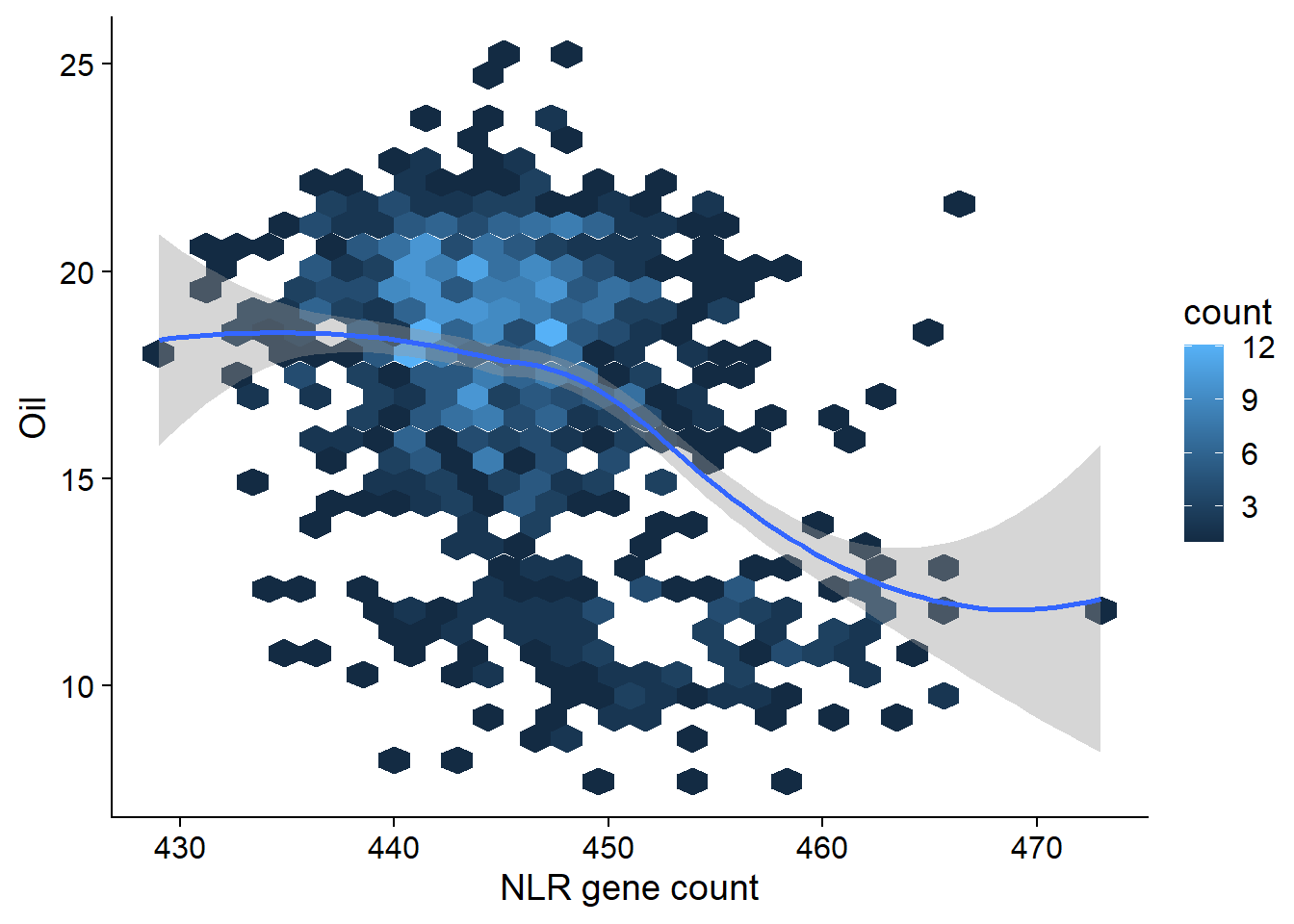
summary(lm(Oil ~ presences, data = oil_join))
Call:
lm(formula = Oil ~ presences, data = oil_join)

Residuals:
     Min       1Q   Median       3Q      Max
-10.4376  -1.9081   0.4846   2.2401   9.0361

Coefficients:
             Estimate Std. Error t value Pr(>|t|)
(Intercept) 118.03941    7.31646   16.13   <2e-16 ***
presences    -0.22591    0.01641  -13.77   <2e-16 ***
---
Signif. codes:  0 '***' 0.001 '**' 0.01 '*' 0.05 '.' 0.1 ' ' 1

Residual standard error: 3.139 on 960 degrees of freedom
Multiple R-squared:  0.1649,    Adjusted R-squared:  0.1641
F-statistic: 189.6 on 1 and 960 DF,  p-value: < 2.2e-16
OK there are many, many outliers here. Clearly I’ll have to do something fancier - for example, using the first two PCs as covariates might get rid of some of those outliers.
Boxplots per group
Yield
nbs_joined_groups %>%
  filter(!is.na(`Group in violin table`)) %>%
  inner_join(yield, by=c('names'='Line')) %>%
  ggplot(aes(x=`Group in violin table`, y=Yield, fill = `Group in violin table`)) +
  geom_boxplot() +
  scale_fill_manual(values = col_list) +
  theme_minimal_hgrid() +
  theme(axis.text.x = element_text(size=12),
        axis.text.y = element_text(size=12)) +
  geom_signif(comparisons = list(c('Old cultivar', 'Modern cultivar')),
              map_signif_level = T) +
  guides(fill=FALSE) +
  ylab('Protein') +
  xlab('Accession group')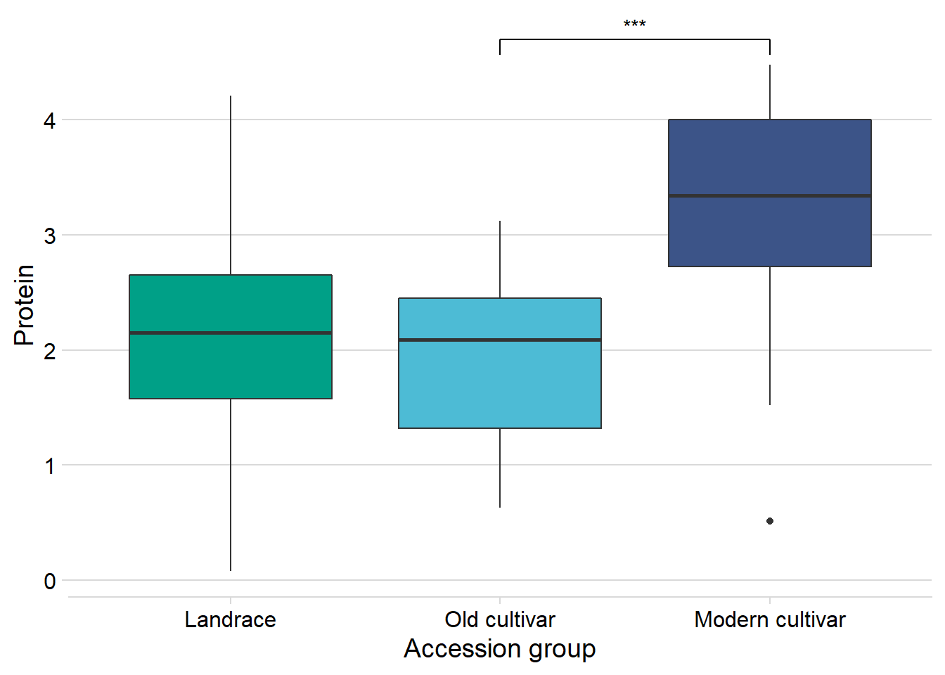
And let’s check the dots:
nbs_joined_groups %>%
  filter(!is.na(`Group in violin table`)) %>%
  inner_join(yield_join, by = 'names') %>%
  ggplot(aes(y=presences.x, x=Yield, color=`Group in violin table`)) +
  geom_point() +
  scale_color_manual(values = col_list) +
  theme_minimal_hgrid() +
  theme(axis.text.x = element_text(size=12),
        axis.text.y = element_text(size=12)) +
  ylab('NLR gene count')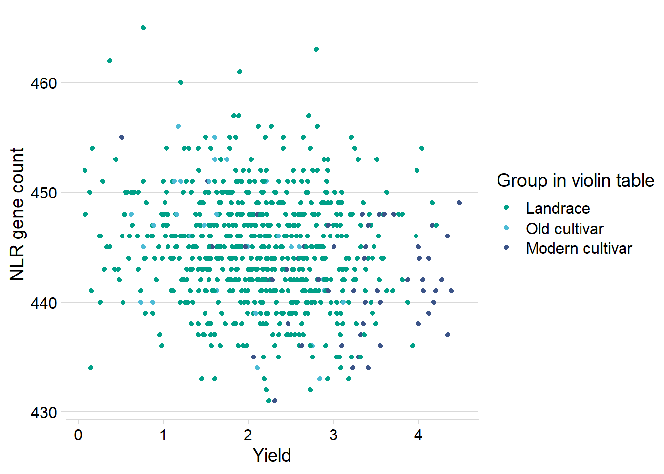
nbs_joined_groups %>%
filter(!is.na(`Group in violin table`)) %>%
inner_join(yield_join, by = 'names') %>%
filter(`Group in violin table` != 'Landrace') %>%
ggplot(aes(x=presences.x, y=Yield, color=`Group in violin table`)) +
geom_point() +
scale_color_manual(values = col_list) +
theme_minimal_hgrid() +
geom_smooth() +
theme(axis.text.x = element_text(size=12),
axis.text.y = element_text(size=12)) +
xlab('NLR gene count')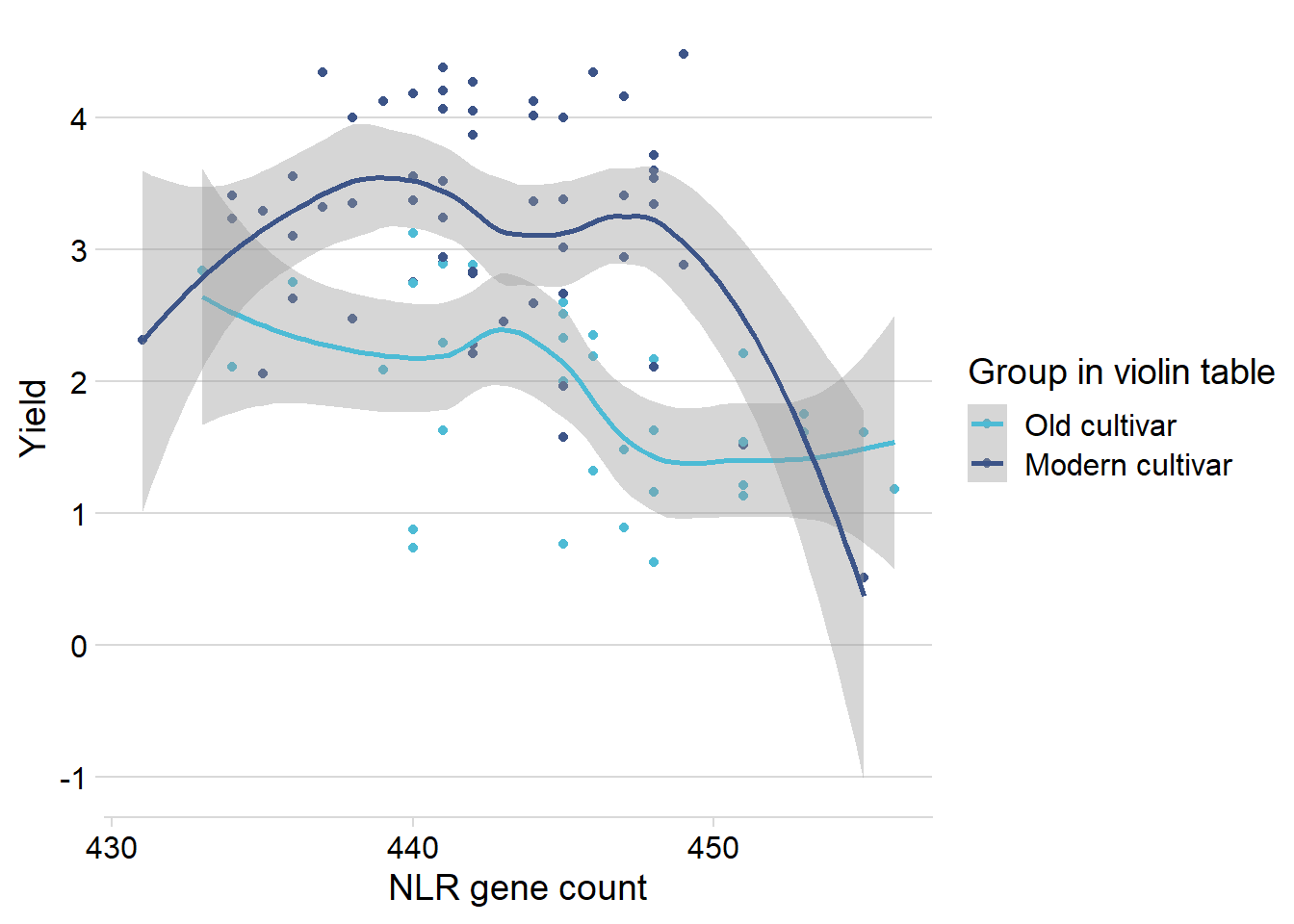 ## Protein
protein vs. the four groups:
nbs_joined_groups %>%
  filter(!is.na(`Group in violin table`)) %>%
  inner_join(protein, by=c('names'='Line')) %>%
  ggplot(aes(x=`Group in violin table`, y=Protein, fill = `Group in violin table`)) +
  geom_boxplot() +
  scale_fill_manual(values = col_list) +
  theme_minimal_hgrid() +
  theme(axis.text.x = element_text(size=12),
        axis.text.y = element_text(size=12)) +
  geom_signif(comparisons = list(c('Wild-type', 'Landrace'),
                                 c('Old cultivar', 'Modern cultivar')),
              map_signif_level = T) +
  guides(fill=FALSE) +
  ylab('Protein') +
  xlab('Accession group')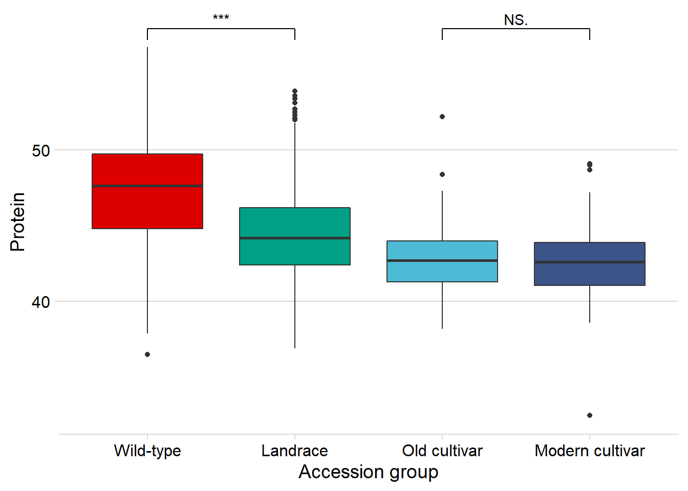
Seed weight
And seed weight:
nbs_joined_groups %>%
  filter(!is.na(`Group in violin table`)) %>%
  inner_join(seed_join) %>%
  ggplot(aes(x=`Group in violin table`, y=wt, fill = `Group in violin table`)) +
  geom_boxplot() +
  scale_fill_manual(values = col_list) +
  theme_minimal_hgrid() +
  theme(axis.text.x = element_text(size=12),
        axis.text.y = element_text(size=12)) +
  geom_signif(comparisons = list(c('Wild-type', 'Landrace'),
                                 c('Old cultivar', 'Modern cultivar')),
              map_signif_level = T) +
  guides(fill=FALSE) +
  ylab('Seed weight') +
  xlab('Accession group')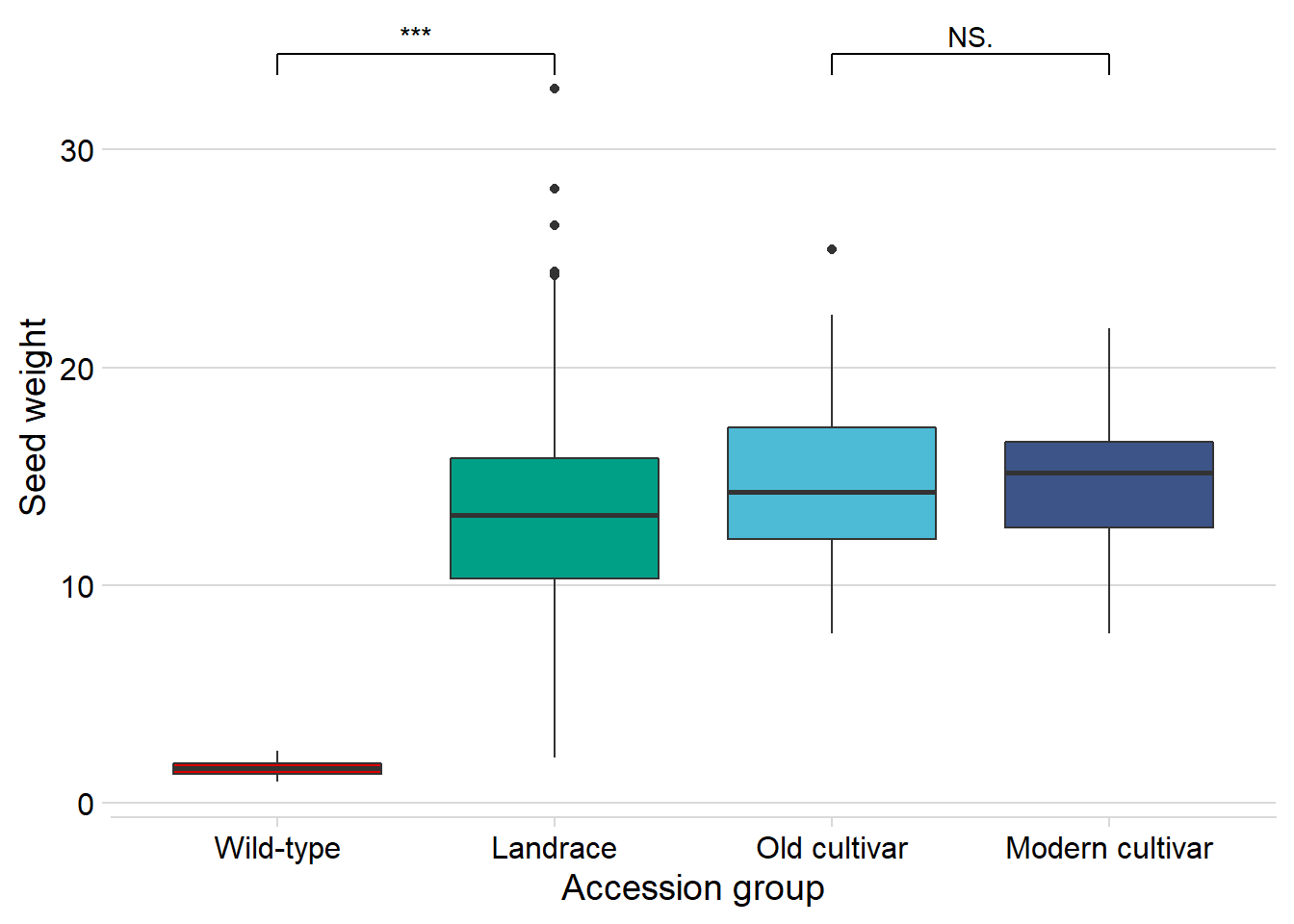
Wow, that’s breeding!
Oil content
And finally, Oil content:
nbs_joined_groups %>%
  filter(!is.na(`Group in violin table`)) %>%
  inner_join(oil_join, by = 'names') %>%
  ggplot(aes(x=`Group in violin table`, y=Oil, fill = `Group in violin table`)) +
  geom_boxplot() +
  scale_fill_manual(values = col_list) +
  theme_minimal_hgrid() +
  theme(axis.text.x = element_text(size=12),
        axis.text.y = element_text(size=12)) +
  geom_signif(comparisons = list(c('Wild-type', 'Landrace'),
                                 c('Old cultivar', 'Modern cultivar')),
              map_signif_level = T) +
  guides(fill=FALSE) +
  ylab('Oil content') +
  xlab('Accession group')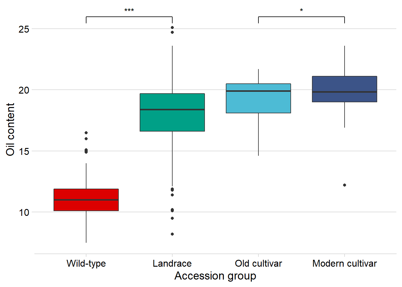
Oha, a single star. That’s p < 0.05!
Let’s redo the above hexplot, but also color the dots by group.
nbs_joined_groups %>%
  filter(!is.na(`Group in violin table`)) %>%
  inner_join(oil_join, by = 'names') %>%
  ggplot(aes(x=presences.x, y=Oil, color=`Group in violin table`)) +
  geom_point() +
  scale_color_manual(values = col_list) +
  theme_minimal_hgrid() +
  theme(axis.text.x = element_text(size=12),
        axis.text.y = element_text(size=12)) +
  xlab('NLR gene count')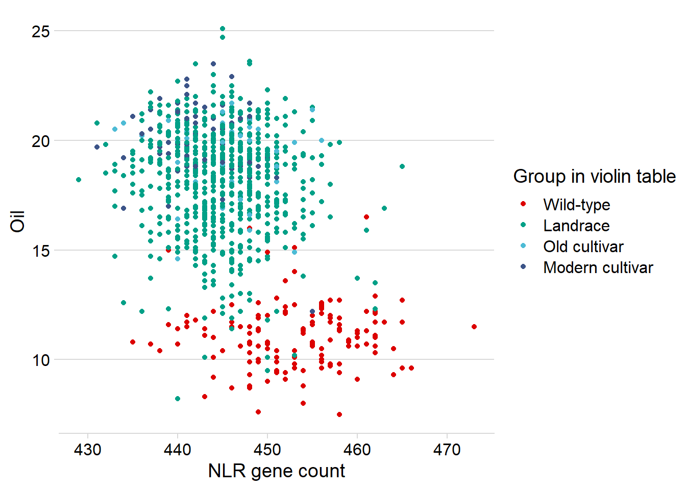
Oha, so it’s the wild-types that drag this out a lot.
Let’s remove them and see what it looks like:
nbs_joined_groups %>%
  filter(!is.na(`Group in violin table`)) %>%
  inner_join(oil_join, by = 'names') %>%
  filter(`Group in violin table` %in% c('Old cultivar', 'Modern cultivar')) %>%
  ggplot(aes(x=presences.x, y=Oil, color=`Group in violin table`)) +
  geom_point() +
  scale_color_manual(values = col_list) +
  theme_minimal_hgrid() +
  theme(axis.text.x = element_text(size=12),
        axis.text.y = element_text(size=12)) +
  xlab('NLR gene count') +
  geom_smooth()
Let’s remove that one outlier:
nbs_joined_groups %>%
  filter(!is.na(`Group in violin table`)) %>%
  inner_join(oil_join, by = 'names') %>%
  filter(`Group in violin table` %in% c('Old cultivar', 'Modern cultivar')) %>%
  filter(Oil > 13) %>%
  ggplot(aes(x=presences.x, y=Oil, color=`Group in violin table`)) +
  geom_point() +
  scale_color_manual(values = col_list) +
  theme_minimal_hgrid() +
  theme(axis.text.x = element_text(size=12),
        axis.text.y = element_text(size=12)) +
  xlab('NLR gene count') +
  geom_smooth()
Does the above oil content boxplot become different if we exclude the one outlier? I’d bet so
nbs_joined_groups %>%
  filter(!is.na(`Group in violin table`)) %>%
  inner_join(oil_join, by = 'names') %>%
  filter(names != 'USB-393') %>%
  ggplot(aes(x=`Group in violin table`, y=Oil, fill = `Group in violin table`)) +
  geom_boxplot() +
  scale_fill_manual(values = col_list) +
  theme_minimal_hgrid() +
  theme(axis.text.x = element_text(size=12),
        axis.text.y = element_text(size=12)) +
  geom_signif(comparisons = list(c('Wild-type', 'Landrace'),
                                 c('Old cultivar', 'Modern cultivar')),
              map_signif_level = T) +
  guides(fill=FALSE) +
  ylab('Oil content') +
  xlab('Accession group')
Nope, still significantly higher in modern cultivars!
sessionInfo()R version 3.6.3 (2020-02-29)
Platform: x86_64-w64-mingw32/x64 (64-bit)
Running under: Windows 10 x64 (build 17134)
Matrix products: default
locale:
[1] LC_COLLATE=English_Australia.1252 LC_CTYPE=English_Australia.1252
[3] LC_MONETARY=English_Australia.1252 LC_NUMERIC=C
[5] LC_TIME=English_Australia.1252
attached base packages:
[1] stats graphics grDevices utils datasets methods base
other attached packages:
[1] ggforce_0.3.1 ggsignif_0.6.0 cowplot_1.0.0
[4] dabestr_0.3.0 magrittr_1.5 ggsci_2.9
[7] patchwork_1.0.0 forcats_0.5.0 stringr_1.4.0
[10] dplyr_1.0.0 purrr_0.3.4 readr_1.3.1
[13] tidyr_1.1.0 tibble_3.0.2 ggplot2_3.3.2
[16] tidyverse_1.3.0 workflowr_1.6.2.9000
loaded via a namespace (and not attached):
[1] httr_1.4.2 jsonlite_1.7.1 splines_3.6.3 modelr_0.1.8
[5] assertthat_0.2.1 getPass_0.2-2 blob_1.2.1 cellranger_1.1.0
[9] yaml_2.2.1 pillar_1.4.4 backports_1.1.10 lattice_0.20-41
[13] glue_1.4.2 digest_0.6.25 promises_1.1.1 polyclip_1.10-0
[17] rvest_0.3.5 colorspace_1.4-1 Matrix_1.2-18 htmltools_0.5.0
[21] httpuv_1.5.4 pkgconfig_2.0.3 broom_0.5.6 haven_2.3.1
[25] scales_1.1.1 processx_3.4.4 tweenr_1.0.1 whisker_0.4
[29] later_1.1.0.1 git2r_0.27.1 mgcv_1.8-31 generics_0.0.2
[33] farver_2.0.3 ellipsis_0.3.1 withr_2.2.0 hexbin_1.28.1
[37] cli_2.0.2 crayon_1.3.4 readxl_1.3.1 evaluate_0.14
[41] ps_1.3.4 fs_1.5.0.9000 fansi_0.4.1 nlme_3.1-148
[45] MASS_7.3-51.6 xml2_1.3.2 tools_3.6.3 hms_0.5.3
[49] lifecycle_0.2.0 munsell_0.5.0 reprex_0.3.0 callr_3.4.4
[53] compiler_3.6.3 rlang_0.4.7 grid_3.6.3 rstudioapi_0.11
[57] labeling_0.3 rmarkdown_2.3 boot_1.3-25 gtable_0.3.0
[61] DBI_1.1.0 R6_2.4.1 lubridate_1.7.9 knitr_1.29
[65] utf8_1.1.4 rprojroot_1.3-2 stringi_1.5.3 Rcpp_1.0.5
[69] vctrs_0.3.1 dbplyr_1.4.4 tidyselect_1.1.0 xfun_0.17