Simulation - Reduced report (results presented in the main paper)
Pedro L. Baldoni
17 February, 2023
Last updated: 2023-02-17
Checks: 5 2
Knit directory: wf-TranscriptDE/analysis/
This reproducible R Markdown analysis was created with workflowr (version 1.7.0). The Checks tab describes the reproducibility checks that were applied when the results were created. The Past versions tab lists the development history.
The R Markdown file has unstaged changes. To know which version of
the R Markdown file created these results, you’ll want to first commit
it to the Git repo. If you’re still working on the analysis, you can
ignore this warning. When you’re finished, you can run
wflow_publish to commit the R Markdown file and build the
HTML.
Great job! The global environment was empty. Objects defined in the global environment can affect the analysis in your R Markdown file in unknown ways. For reproduciblity it’s best to always run the code in an empty environment.
The command set.seed(20221115) was run prior to running
the code in the R Markdown file. Setting a seed ensures that any results
that rely on randomness, e.g. subsampling or permutations, are
reproducible.
Great job! Recording the operating system, R version, and package versions is critical for reproducibility.
- simulation-paper_data_load
To ensure reproducibility of the results, delete the cache directory
simulation-paper_cache and re-run the analysis. To have
workflowr automatically delete the cache directory prior to building the
file, set delete_cache = TRUE when running
wflow_build() or wflow_publish().
Great job! Using relative paths to the files within your workflowr project makes it easier to run your code on other machines.
Great! You are using Git for version control. Tracking code development and connecting the code version to the results is critical for reproducibility.
The results in this page were generated with repository version 60067c3. See the Past versions tab to see a history of the changes made to the R Markdown and HTML files.
Note that you need to be careful to ensure that all relevant files for
the analysis have been committed to Git prior to generating the results
(you can use wflow_publish or
wflow_git_commit). workflowr only checks the R Markdown
file, but you know if there are other scripts or data files that it
depends on. Below is the status of the Git repository when the results
were generated:
Ignored files:
    Ignored:    .DS_Store
    Ignored:    .Rhistory
    Ignored:    .Rproj.user/
    Ignored:    ._.DS_Store
    Ignored:    .gitignore
    Ignored:    analysis/simulation-complete_cache/
    Ignored:    analysis/simulation-paper_cache/
    Ignored:    code/mouse/single-end/salmon/slurm-9574761.out
    Ignored:    code/pkg/.Rhistory
    Ignored:    code/pkg/.Rproj.user/
    Ignored:    code/pkg/src/RcppExports.o
    Ignored:    code/pkg/src/pkg.so
    Ignored:    code/pkg/src/rcpparma_hello_world.o
    Ignored:    data/annotation/mm39/
    Ignored:    data/mouse/paired-end/fastq/
    Ignored:    data/mouse/single-end/fastq/
    Ignored:    misc/.DS_Store
    Ignored:    misc/._.DS_Store
    Ignored:    misc/mouse.Rmd/._figure6.png
    Ignored:    misc/simulation-paper.Rmd/._figure2.png
    Ignored:    misc/simulation-paper.Rmd/._figure5.png
    Ignored:    output/mouse/paired-end/
    Ignored:    output/mouse/single-end/
    Ignored:    output/quasi_poisson/
    Ignored:    output/simulation/

Untracked files:
    Untracked:  analysis/simulation-howto.Rmd
    Untracked:  misc/bibliography/

Unstaged changes:
    Modified:   analysis/index.Rmd
    Modified:   analysis/license.Rmd
    Modified:   analysis/mouse.Rmd
    Modified:   analysis/simulation-complete.Rmd
    Modified:   analysis/simulation-paper.Rmd
Note that any generated files, e.g. HTML, png, CSS, etc., are not included in this status report because it is ok for generated content to have uncommitted changes.
These are the previous versions of the repository in which changes were
made to the R Markdown (analysis/simulation-paper.Rmd) and
HTML (docs/simulation-paper.html) files. If you’ve
configured a remote Git repository (see ?wflow_git_remote),
click on the hyperlinks in the table below to view the files as they
were in that past version.
| File | Version | Author | Date | Message |
|---|---|---|---|---|
| Rmd | 623d429 | Pedro Baldoni | 2023-01-23 | Splitting figures |
| html | 623d429 | Pedro Baldoni | 2023-01-23 | Splitting figures |
| Rmd | 49c9a94 | Pedro Baldoni | 2023-01-19 | Expanding panels to multiple figures |
| html | 49c9a94 | Pedro Baldoni | 2023-01-19 | Expanding panels to multiple figures |
| Rmd | 4276bfc | Pedro Baldoni | 2023-01-06 | Organizing output of latex table |
| html | 4276bfc | Pedro Baldoni | 2023-01-06 | Organizing output of latex table |
| Rmd | a8c51af | Pedro Baldoni | 2023-01-05 | Updating simulation-paper report |
| html | a8c51af | Pedro Baldoni | 2023-01-05 | Updating simulation-paper report |
| Rmd | d34d4e6 | Pedro Baldoni | 2022-11-24 | Adding simulation-paper-report |
| html | d34d4e6 | Pedro Baldoni | 2022-11-24 | Adding simulation-paper-report |
Introduction
In this report, we present the analysis of the simulations for the
catchSalmon/catchKallisto manuscript. These
simulations aim to generate typical RNA-seq data from mouse experiments.
This report focuses on the results presented in the main paper only. For
a comprehensive report of the results, please refer to the complete report.
Setup
We load necessary libraries and set up the rendering options below.
knitr::opts_chunk$set(dev = "png",
                      dpi = 300,
                      dev.args = list(type = "cairo-png"),
                      root.dir = '.',
                      autodep = TRUE)

options(knitr.kable.NA = "-")
library(data.table)
library(ggplot2)
library(thematic)
library(plyr)
library(magrittr)
library(limma)
library(edgeR)
library(BiocParallel)
library(devtools)
library(purrr)
library(readr)
library(ggpubr)
library(kableExtra)
library(patchwork)
library(ragg)
load_all('../code/pkg/')I use the functions below to produce the histogram plot shown in this report and to quickly subset data tables for specific scenarios.
cleanPlot <- function(x,fig){
  if (x == max(seq_along(fig))) {
    y <- fig[[x]]
  } else{
    y <- fig[[x]] + theme(axis.title.x = element_blank(),
                          axis.text.x = element_blank(),
                          axis.ticks.x = element_blank())
  }
  if (x > 1) {
    y <- y + theme(strip.background.x = element_blank(),
                   strip.text.x = element_blank())
  }
  return(y)
}

subsetDT <- function(x,scenario,panel = NULL,tx.per.gene = NULL, plot = TRUE){
  if(isTRUE(plot)){
    if(panel %in% c('A','B')){
      out <- x[Genome == scenario['genome'] &
                 FC == ifelse(panel == 'A','fc2','fc1') &
                 Length == scenario['length'] &
                 Reads == scenario['read'] &
                 Quantifier == scenario['quantifier'] &
                 Scenario == scenario['scenario'],]
    } else{
      out <- x[Genome == scenario['genome'] &
                 FC == 'fc1' &
                 Length == scenario['length'] &
                 Reads == scenario['read'] &
                 Quantifier == scenario['quantifier'] &
                 Scenario == scenario['scenario'] &
                 TxPerGene == tx.per.gene ,]
    }
  } else{
    out <- x[Genome == scenario['genome'] &
               FC == 'fc2' &
               Quantifier == scenario['quantifier'] &
               TxPerGene == scenario['txpergene'],]
  }
  return(out)
}
Analysis
Here we begin summarizing the results to generate the figures presented in the main paper.
Data wrangling
Below I set up the file paths.
path.misc <- file.path('../misc',knitr::current_input())
dir.create(path.misc,recursive = TRUE,showWarnings = FALSE)

path.fdr <-
  list.files('../output/simulation/summary','fdr.tsv.gz',recursive = TRUE,full.names = TRUE)
path.metrics <-
  list.files('../output/simulation/summary','metrics.tsv.gz',recursive = TRUE,full.names = TRUE)
path.time <-
  list.files('../output/simulation/summary','time.tsv.gz',recursive = TRUE,full.names = TRUE)
path.quantile <-
  list.files('../output/simulation/summary','quantile.tsv.gz',recursive = TRUE,full.names = TRUE)
path.pvalue <-
  list.files('../output/simulation/summary','pvalue.tsv.gz',recursive = TRUE,full.names = TRUE)
path.overdispersion <-
  list.files('../output/simulation/summary','overdispersion.tsv.gz',recursive = TRUE,full.names = TRUE)
Loading all summarized results below. Because these datasets are
quite large, I use cache=TRUE to save time when rendering
this page.
# Loading datasets
dt.fdr <- do.call(rbind,lapply(path.fdr,fread))
dt.metrics <- do.call(rbind,lapply(path.metrics,fread))
dt.time <- do.call(rbind,lapply(path.time,fread))
dt.quantile <- do.call(rbind,lapply(path.quantile,fread))
dt.pvalue <- do.call(rbind,lapply(path.pvalue,fread))
dt.overdispersion <- do.call(rbind,lapply(path.overdispersion,fread))
Some data wrangling below.
# Changing labels
dt.fdr$TxPerGene %<>%
  mapvalues(from = paste0(c(2, 3, 4, 5, 9999), 'TxPerGene'),
            to = c(paste0("#Tx/Gene = ", c(2, 3, 4, 5)), 'All Transcripts'))
dt.fdr$LibsPerGroup %<>%
  mapvalues(from = paste0(c(3, 5), 'libsPerGroup'),
            to = paste0('#Lib/Group = ', c(3, 5)))
dt.fdr$Quantifier %<>% mapvalues(from = 'salmon', to = 'Salmon')
dt.fdr$Length %<>% mapvalues(from = paste0('readlen-', seq(50, 150, 25)),
                             to = paste0(seq(50, 150, 25), 'bp'))

dt.metrics$TxPerGene %<>%
  mapvalues(from = paste0(c(2, 3, 4, 5, 9999), 'TxPerGene'),
            to = c(paste0("#Tx/Gene = ", c(2, 3, 4, 5)), 'All Transcripts'))
dt.metrics$LibsPerGroup %<>%
  mapvalues(from = paste0(c(3, 5), 'libsPerGroup'),
            to = paste0('#Lib/Group = ', c(3, 5)))
dt.metrics$Quantifier %<>% mapvalues(from = 'salmon', to = 'Salmon')
dt.metrics$Length %<>% mapvalues(from = paste0('readlen-', seq(50, 150, 25)),
                                 to = paste0(seq(50, 150, 25), 'bp'))

dt.time$TxPerGene %<>%
  mapvalues(from = paste0(c(2, 3, 4, 5, 9999), 'TxPerGene'),
            to = c(paste0("#Tx/Gene = ", c(2, 3, 4, 5)), 'All Transcripts'))
dt.time$LibsPerGroup %<>%
  mapvalues(from = paste0(c(3, 5), 'libsPerGroup'),
            to = paste0('#Lib/Group = ', c(3, 5)))
dt.time$Quantifier %<>% mapvalues(from = 'salmon', to = 'Salmon')
dt.time$Length %<>% mapvalues(from = paste0('readlen-', seq(50, 150, 25)),
                              to = paste0(seq(50, 150, 25), 'bp'))

dt.quantile$TxPerGene %<>%
  mapvalues(from = paste0(c(2, 3, 4, 5, 9999), 'TxPerGene'),
            to = c(paste0("#Tx/Gene = ", c(2, 3, 4, 5)), 'All Transcripts'))
dt.quantile$LibsPerGroup %<>%
  mapvalues(from = paste0(c(3, 5), 'libsPerGroup'),
            to = paste0('#Lib/Group = ', c(3, 5)))
dt.quantile$Quantifier %<>% mapvalues(from = 'salmon', to = 'Salmon')
dt.quantile$Length %<>% mapvalues(from = paste0('readlen-', seq(50, 150, 25)),
                                  to = paste0(seq(50, 150, 25), 'bp'))

dt.pvalue$TxPerGene %<>%
  mapvalues(from = paste0(c(2, 3, 4, 5, 9999), 'TxPerGene'),
            to = c(paste0("#Tx/Gene = ", c(2, 3, 4, 5)), 'All Transcripts'))
dt.pvalue$LibsPerGroup %<>%
  mapvalues(from = paste0(c(3, 5), 'libsPerGroup'),
            to = paste0('#Lib/Group = ', c(3, 5)))
dt.pvalue$Quantifier %<>% mapvalues(from = 'salmon', to = 'Salmon')
dt.pvalue$Length %<>% mapvalues(from = paste0('readlen-', seq(50, 150, 25)),
                                to = paste0(seq(50, 150, 25), 'bp'))

dt.overdispersion$TxPerGene %<>%
  mapvalues(from = paste0(c(2, 3, 4, 5, 9999), 'TxPerGene'),
            to = c(paste0("#Tx/Gene = ", c(2, 3, 4, 5)), 'All Transcripts'))
dt.overdispersion$LibsPerGroup %<>%
  mapvalues(from = paste0(c(3, 5), 'libsPerGroup'),
            to = paste0('#Lib/Group = ', c(3, 5)))
dt.overdispersion$Quantifier %<>% mapvalues(from = 'salmon', to = 'Salmon')
dt.overdispersion$Length %<>% mapvalues(from = paste0('readlen-', seq(50, 150, 25)),
                                        to = paste0(seq(50, 150, 25), 'bp'))
All the simulated scenarios are generated below.
dt.scenario <- expand.grid('genome' = 'mm39',
                           'length' = c('50bp','75bp','100bp','125bp','150bp'),
                           'read' = c('single-end','paired-end'),
                           'quantifier' = c('Salmon','kallisto'),
                           'scenario' = c('balanced','unbalanced'),
                           stringsAsFactors = FALSE)
dt.scenario <- as.data.table(dt.scenario)
Power plot & False discovery rate
Below we generate Figure 2 of the main paper.
scenario.balanced <- as.character(dt.scenario[length == '100bp' &
                                                read == 'paired-end' &
                                                quantifier == 'Salmon' &
                                                scenario == 'balanced',])
scenario.unbalanced <- as.character(dt.scenario[length == '100bp' &
                                                  read == 'paired-end' &
                                                  quantifier == 'Salmon' &
                                                  scenario == 'unbalanced',])
names(scenario.balanced) <- colnames(dt.scenario)
names(scenario.unbalanced) <- colnames(dt.scenario)


dt.power <- rbind(subsetDT(dt.metrics,scenario.balanced,'A'),
                  subsetDT(dt.metrics,scenario.unbalanced,'A'))

dt.power$LibsPerGroup %<>% mapvalues(from = paste0('#Lib/Group = ', c(3, 5)),
                                     to = paste0(c(3,5),' samples per group'))

dt.power$Scenario %<>%
  mapvalues(from = c('balanced','unbalanced'),
            to = c('Equal library sizes','Unequal library sizes'))

dt.power[, FDR := roundPretty(ifelse((FP+TP) == 0,NA,100*FP/(FP+TP)),1)]

dt.power <- dt.power[TxPerGene == 'All Transcripts',]

sub.byvar <-
  colnames(dt.power)[-which(colnames(dt.power) %in% c('P.SIG','TP','FP'))]

gap <- 0.05*max(dt.power$TP + dt.power$FP)

x.melt <- melt(dt.power,id.vars = sub.byvar,
               measure.vars = c('TP','FP'),
               variable.name = 'Type',
               value.name = 'Value')
x.melt$Type <-
  factor(x.melt$Type,
         levels = c('FP','TP'),
         labels = c('False','True'))

plot.power <- function(df.bar,df.txt,scenario,library,legend = FALSE, base_size = 8){
  tb.bar <- df.bar[Scenario == scenario & LibsPerGroup == library,]
  tb.txt <- df.txt[Scenario == scenario & LibsPerGroup == library,][FDR != 'NA',]

  ggplot(tb.bar,aes(x = Method,y = Value,fill = Type)) +
    geom_col(colour = 'black') +
    geom_text(aes(x = Method,y = (TP + FP) + gap,label = FDR),
              vjust = 0,data = tb.txt,size = base_size/.pt,inherit.aes = FALSE) +
    scale_fill_manual(values = c('#ff0000','#bebebe')) +
    labs(x = NULL,y = paste('DE Transcripts')) +
    scale_y_continuous(limits = c(0,3000)) +
    theme_bw(base_size = base_size,base_family = 'sans') +
    theme(panel.grid = element_blank(),
          axis.text.x = element_text(angle = 90),
          axis.text = element_text(colour = 'black',size = base_size)) +
    if (legend == TRUE) theme(legend.background = element_rect(fill = alpha('white', 0)),
                              legend.text = element_text(size = base_size),
                              legend.position = c(0.80,0.90),legend.title = element_blank(),
                              legend.key.size = unit(0.75,"line")) else theme(legend.position = 'none')
}

fig.power.a <- plot.power(df.bar = x.melt,df.txt = dt.power,scenario = 'Equal library sizes',library = '3 samples per group')
fig.power.b <- plot.power(df.bar = x.melt,df.txt = dt.power,scenario = 'Unequal library sizes',library = '3 samples per group',legend = TRUE)
fig.power.c <- plot.power(df.bar = x.melt,df.txt = dt.power,scenario = 'Equal library sizes',library = '5 samples per group')
fig.power.d <- plot.power(df.bar = x.melt,df.txt = dt.power,scenario = 'Unequal library sizes',library = '5 samples per group')

fig.power <- (fig.power.a + fig.power.b) / (fig.power.c + fig.power.d) +
  plot_annotation(tag_levels = 'a') +
  theme(plot.tag = element_text(size = 8))

agg_png(filename = file.path(path.misc,"figure2.png"),width = 5,height = 5,units = 'in',res = 300)
fig.power
dev.off()
png
2 fig.power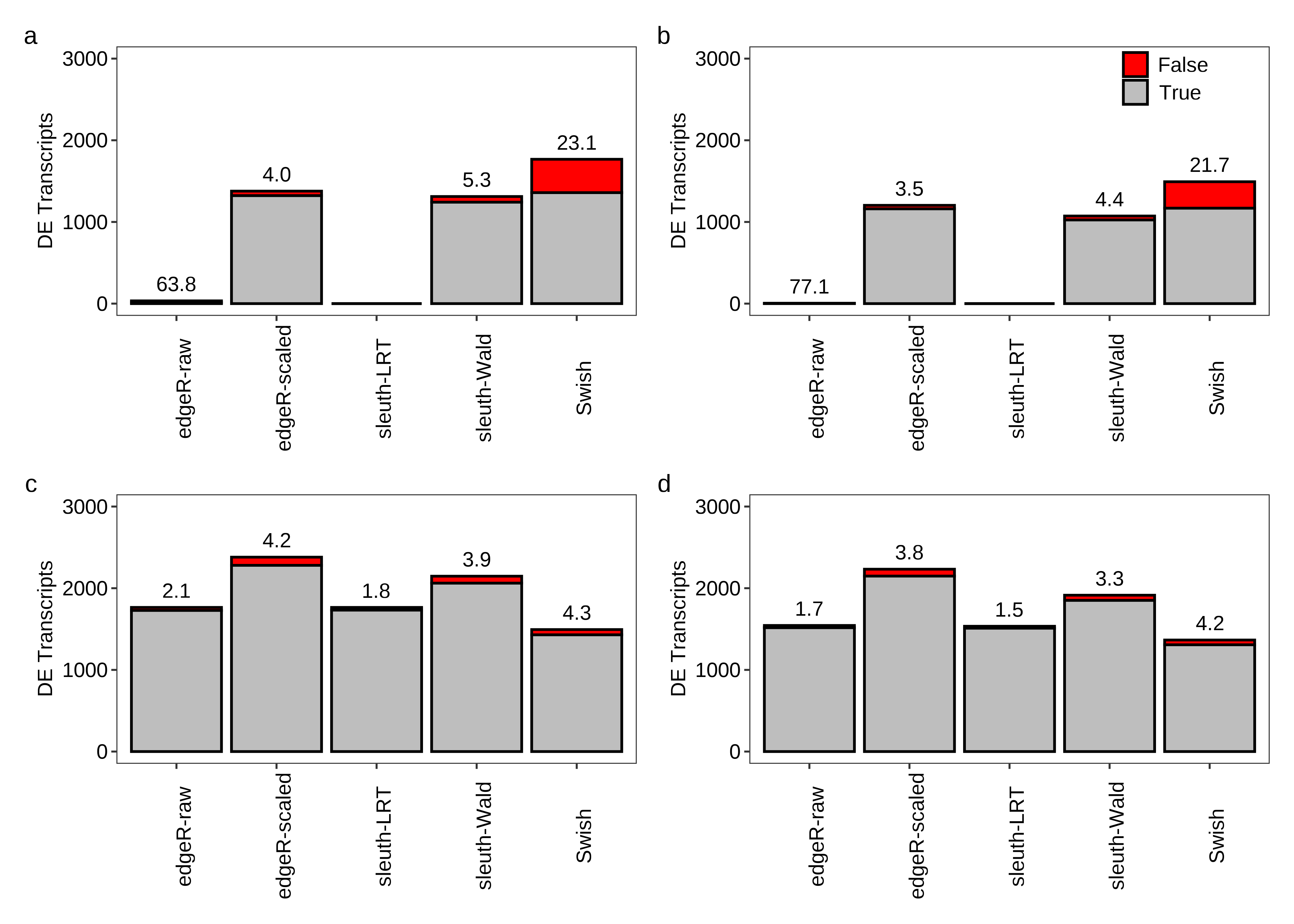
Then, we generate Figure 3 below.
dt.fdr.plot <- rbind(subsetDT(dt.fdr,scenario.balanced,'A'),
                     subsetDT(dt.fdr,scenario.unbalanced,'A'))

dt.fdr.plot$LibsPerGroup %<>%
  mapvalues(from = paste0('#Lib/Group = ', c(3, 5)),
            to = paste0(c(3,5),' samples per group'))

dt.fdr.plot$Scenario %<>%
  mapvalues(from = c('balanced','unbalanced'),
            to = c('Equal library sizes','Unequal library sizes'))

dt.fdr.plot <- dt.fdr.plot[TxPerGene == 'All Transcripts',]

plot.fdr <- function(df.line,scenario,library,legend = FALSE,base_size = 8){
  tb.bar <- df.line[Scenario == scenario & LibsPerGroup == library,]

  ggplot(tb.bar,aes(x = N,y = FDR,color = Method,group = Method)) +
    geom_line(linewidth = 0.5) +
    scale_color_manual(values = methodsNames()$color) +
    scale_y_continuous(limits = c(0,1250)) +
    labs(y = 'False discoveries',x = 'Transcripts chosen') +
    theme_bw(base_size = base_size,base_family = 'sans') +
    theme(panel.grid = element_blank(),
          axis.text = element_text(colour = 'black',size = base_size)) +
    if (legend == TRUE) theme(legend.background = element_rect(fill = alpha('white', 0)),
                              legend.direction = 'vertical',
                              legend.position = c(0.3,0.8),
                              legend.text = element_text(size = base_size),
                              legend.title = element_blank(),
                              legend.key.size = unit(0.75,"line")) else theme(legend.position = 'none')
}

fig.fdr.a <- plot.fdr(df.line = dt.fdr.plot,scenario = 'Equal library sizes',library = '3 samples per group')
fig.fdr.b <- plot.fdr(df.line = dt.fdr.plot,scenario = 'Unequal library sizes',library = '3 samples per group',legend = TRUE)
fig.fdr.c <- plot.fdr(df.line = dt.fdr.plot,scenario = 'Equal library sizes',library = '5 samples per group')
fig.fdr.d <- plot.fdr(df.line = dt.fdr.plot,scenario = 'Unequal library sizes',library = '5 samples per group')

fig.fdr <- (fig.fdr.a + fig.fdr.b) / (fig.fdr.c + fig.fdr.d) +
  plot_annotation(tag_levels = 'a')

agg_png(filename = file.path(path.misc,"figure3.png"),width = 5,height = 5,units = 'in',res = 300)
fig.fdr
dev.off()
png
2 fig.fdr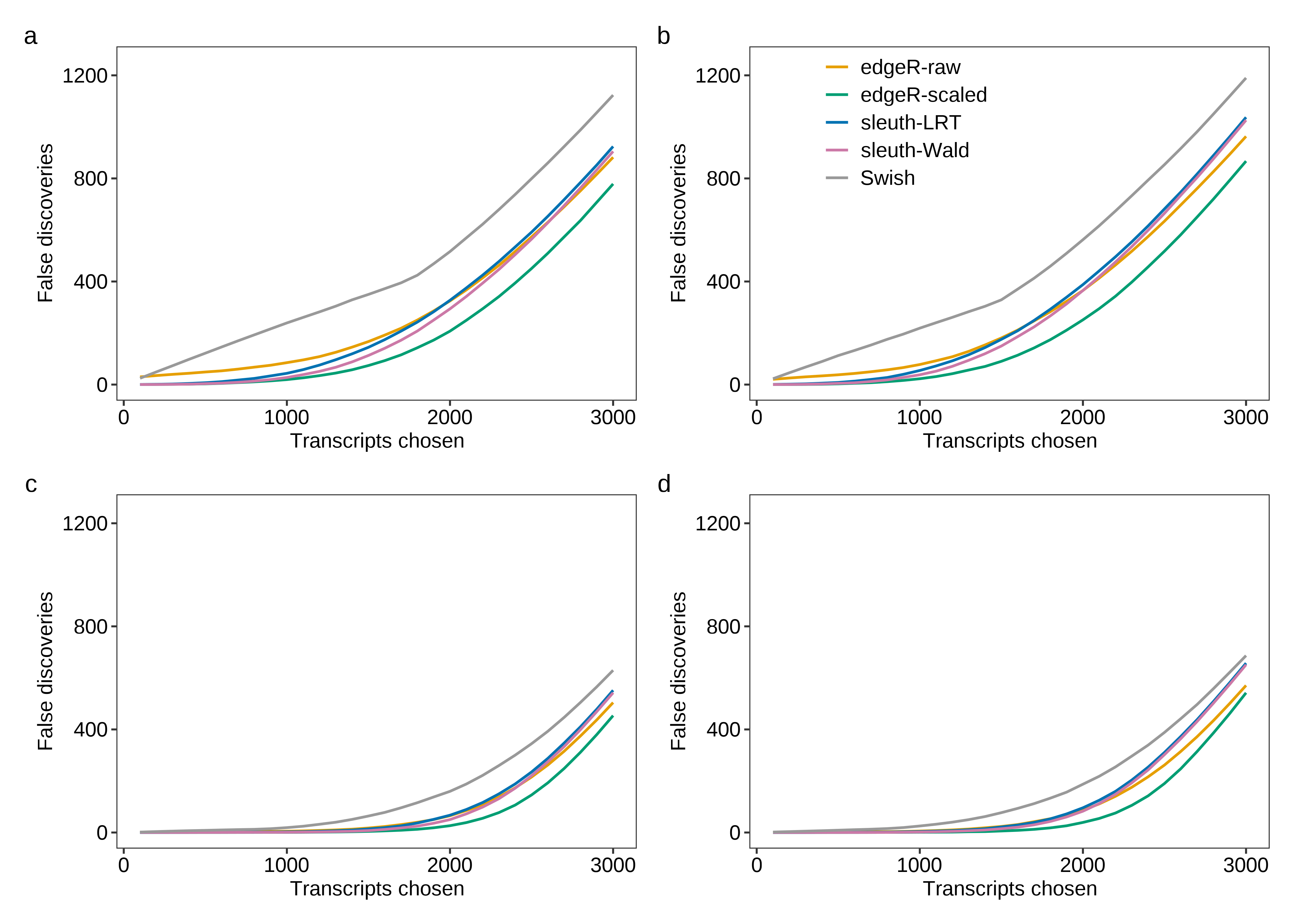
Type 1 error
Figure 4 is created below.
dt.type1error <- rbind(subsetDT(dt.metrics,scenario.balanced,'B'),
                       subsetDT(dt.metrics,scenario.unbalanced,'B'))

dt.type1error$LibsPerGroup %<>%
  mapvalues(from = paste0('#Lib/Group = ', c(3, 5)),
            to = paste0(c(3,5),' samples per group'))

dt.type1error$Scenario %<>%
  mapvalues(from = c('balanced','unbalanced'),
            to = c('Equal library sizes','Unequal library sizes'))

dt.type1error[, FDR := roundPretty(ifelse((FP+TP) == 0,NA,100*FP/(FP+TP)),1)]

dt.type1error <- dt.type1error[TxPerGene == 'All Transcripts',]


sub.byvar <-
  colnames(dt.type1error)[-which(colnames(dt.type1error) %in% c('P.SIG','TP','FP'))]

x.melt <-
  melt(dt.type1error,id.vars = sub.byvar,
       measure.vars = c('P.SIG'),variable.name = 'Type',value.name = 'Value')

plot.type1error <- function(df.bar,scenario,library,legend = FALSE,base_size = 8){
  tb.bar <- df.bar[Scenario == scenario & LibsPerGroup == library,]

  ggplot(tb.bar,aes(x = Method,y = Value)) +
    geom_col(fill = "#bebebe",col = 'black') +
    geom_hline(yintercept = 0.05,color = '#ff0000',linetype = 'dashed',linewidth = 0.5) +
    labs(x = NULL,y = paste('Type 1 error rate')) +
    scale_y_continuous(limits = c(0,0.06),breaks = c(0,0.02,0.04,0.06)) +
    theme_bw(base_size = base_size,base_family = 'sans') +
    theme(panel.grid = element_blank(),
          axis.text.x = element_text(angle = 90),
          axis.text = element_text(colour = 'black',size = base_size))
}

fig.type1error.a <- plot.type1error(df.bar = x.melt,scenario = 'Equal library sizes',library = '3 samples per group')
fig.type1error.b <- plot.type1error(df.bar = x.melt,scenario = 'Unequal library sizes',library = '3 samples per group')
fig.type1error.c <- plot.type1error(df.bar = x.melt,scenario = 'Equal library sizes',library = '5 samples per group')
fig.type1error.d <- plot.type1error(df.bar = x.melt,scenario = 'Unequal library sizes',library = '5 samples per group')

fig.type1error <- (fig.type1error.a + fig.type1error.b) / (fig.type1error.c + fig.type1error.d) +
  plot_annotation(tag_levels = 'a')

agg_png(filename = file.path(path.misc,"figure4.png"),width = 5,height = 5,units = 'in',res = 300)
fig.type1error
dev.off()
png
2 fig.type1error
Finally, we generate Figure 5.
dt.pvalue.plot <- subsetDT(dt.pvalue,scenario.unbalanced,'C','All Transcripts')
dt.pvalue.plot <- dt.pvalue.plot[LibsPerGroup == '#Lib/Group = 5',]

plot.hist <- function(df.hist,method,legend = FALSE,base_size = 8){
  tb.bar <- df.hist[Method == method,]

  ggplot(data = tb.bar,aes(x = PValue,y = Density.Avg)) +
    geom_col(fill = "#bebebe",col = 'black',position = position_dodge(),width = 0.75) +
    geom_hline(yintercept = 1,col = '#ff0000',linetype = 'dashed',linewidth = 0.5) +
    scale_x_discrete(breaks = c("(0.00-0.05]","(0.50-0.55]","(0.95-1.00]"),
                     labels = c(0.00,0.50,1.00)) +
    labs(x = 'P-values',y = 'Density') +
    theme_bw(base_size = base_size,base_family = 8) +
    theme(panel.grid = element_blank(),
          axis.text = element_text(colour = 'black',size = base_size))
}

fig.hist.a <- plot.hist(df.hist = dt.pvalue.plot,method = 'edgeR-raw')
fig.hist.b <- plot.hist(df.hist = dt.pvalue.plot,method = 'edgeR-scaled')
fig.hist.c <- plot.hist(df.hist = dt.pvalue.plot,method = 'sleuth-LRT')
fig.hist.d <- plot.hist(df.hist = dt.pvalue.plot,method = 'sleuth-Wald')
fig.hist.e <- plot.hist(df.hist = dt.pvalue.plot,method = 'Swish')

design <- c(
  area(1,1),area(1,2),
  area(2,1),area(2,2),
  area(3,1)
)

fig.hist <- fig.hist.a + fig.hist.b + fig.hist.c + fig.hist.d + fig.hist.e +
  plot_layout(design = design) +
  plot_annotation(tag_levels = 'a')

agg_png(filename = file.path(path.misc,"figure5.png"),width = 5,height = 7.5,units = 'in',res = 300)
fig.hist
dev.off()
png
2 fig.type1error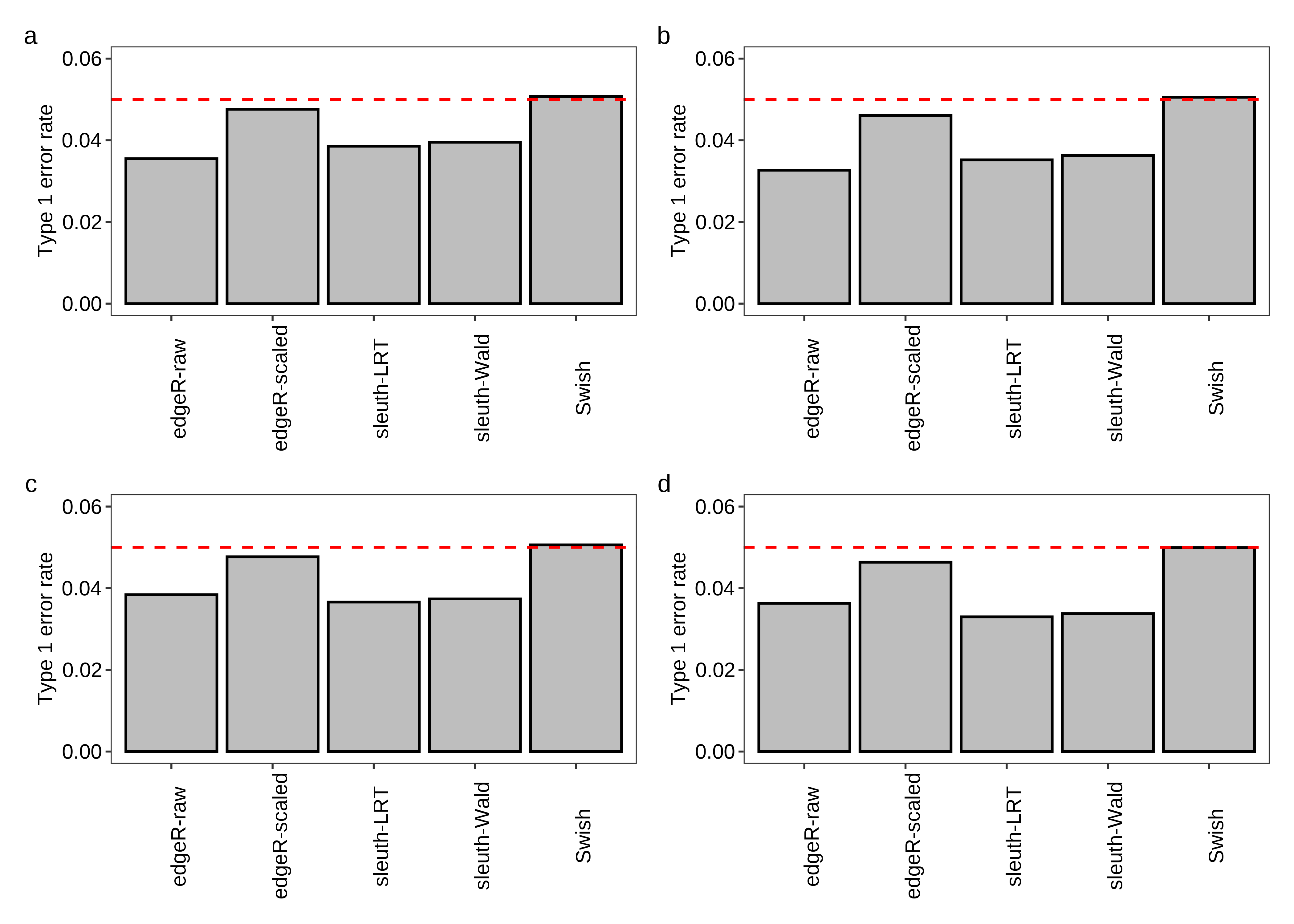
Read type
Below we generate Table 1 of the main paper.
# Overdispersion fold-change
dt.sigma2 <- dt.overdispersion[TxPerGene == 'All Transcripts' &
                                 Quantifier == 'Salmon' &
                                 Scenario == 'unbalanced' &
                                 FC == 'fc2',]

dt.sigma2 <- dt.sigma2[,-c(1,3,5,6,8,10:15)]

dt.sigma2.150.PE <- dt.sigma2[Length == '150bp' & Reads == 'paired-end',][,-c(1,2)]
setnames(dt.sigma2.150.PE,old = 'Mean',new = 'Mean.150.PE')

dt.sigma2 <- merge(dt.sigma2,dt.sigma2.150.PE,by = c('LibsPerGroup'),
                   all.x=TRUE,sort = FALSE)

dt.sigma2[,FC := Mean - Mean.150.PE]

dt.sigma2.3 <- dt.sigma2[LibsPerGroup == '#Lib/Group = 3',]
dt.sigma2.5 <- dt.sigma2[LibsPerGroup == '#Lib/Group = 5',]

dt.sigma2.3 <- dcast(dt.sigma2.3,LibsPerGroup + Length ~ Reads,value.var = 'FC')
dt.sigma2.5 <- dcast(dt.sigma2.5,LibsPerGroup + Length ~ Reads,value.var = 'FC')

setnames(dt.sigma2.3,
         old = c('paired-end','single-end'),
         new = c('FC.PE','FC.SE'))
setnames(dt.sigma2.5,
         old = c('paired-end','single-end'),
         new = c('FC.PE','FC.SE'))

setcolorder(dt.sigma2.3,neworder = c('LibsPerGroup','Length','FC.PE','FC.SE'))
setcolorder(dt.sigma2.5,neworder = c('LibsPerGroup','Length','FC.PE','FC.SE'))

dt.sigma2.long <- rbind(dt.sigma2.3,dt.sigma2.5)
dt.sigma2.long$LibsPerGroup %<>%
  mapvalues(from = c('#Lib/Group = 3','#Lib/Group = 5'),to = c(3,5))
dt.sigma2.long$Length %<>% factor(levels = paste0(seq(50,150,25),'bp'))
dt.sigma2.long <- dt.sigma2.long[order(LibsPerGroup,Length),]

# Power and FDR
dt.scenario.table <-
  expand.grid('genome' = 'mm39',
              'quantifier' = c('Salmon','kallisto'),
              'txpergene' = c(paste0('#Tx/Gene = ',2:5),'All Transcripts'),
              stringsAsFactors = FALSE)

dt.scenario.table <- as.data.table(dt.scenario.table)

scenario.table <-
  dt.scenario.table[quantifier == 'Salmon' & txpergene == 'All Transcripts',]
scenario.table <- as.character(scenario.table)
names(scenario.table) <- colnames(dt.scenario.table)

dt.table <- subsetDT(dt.metrics,scenario = scenario.table,plot = FALSE)
dt.table <- dt.table[Method == 'edgeR-scaled' &
                       Scenario == 'unbalanced',]

dt.table[,Power := TP/3000]
dt.table[,FDR := ifelse((FP+TP) == 0,NA,FP/(FP+TP))]

dt.table.3 <- dt.table[LibsPerGroup == '#Lib/Group = 3',][,-c(1,3,5,6,8:12)]
dt.table.5 <- dt.table[LibsPerGroup == '#Lib/Group = 5',][,-c(1,3,5,6,8:12)]

dt.table.3 <- dcast(dt.table.3,LibsPerGroup + Length ~ Reads,value.var = c('Power','FDR'))
dt.table.5 <- dcast(dt.table.5,LibsPerGroup + Length ~ Reads,value.var = c('Power','FDR'))

setnames(dt.table.3,
         old = c('Power_paired-end','Power_single-end','FDR_paired-end','FDR_single-end'),
         new = c('Power.PE','Power.SE','FDR.PE','FDR.SE'))
setnames(dt.table.5,
         old = c('Power_paired-end','Power_single-end','FDR_paired-end','FDR_single-end'),
         new = c('Power.PE','Power.SE','FDR.PE','FDR.SE'))

setcolorder(dt.table.3,neworder = c('LibsPerGroup','Length','Power.SE','FDR.SE','Power.PE','FDR.PE'))
setcolorder(dt.table.5,neworder = c('LibsPerGroup','Length','Power.SE','FDR.SE','Power.PE','FDR.PE'))

dt.table.long <- rbind(dt.table.3,dt.table.5)
dt.table.long$LibsPerGroup %<>% mapvalues(from = c('#Lib/Group = 3','#Lib/Group = 5'),to = c(3,5))
dt.table.long$Length %<>% factor(levels = paste0(seq(50,150,25),'bp'))
dt.table.long <- dt.table.long[order(LibsPerGroup,Length),]

# Organizing tables

dt.table.sigma2 <-
  merge(dt.table.long,dt.sigma2.long,
        all.x = TRUE,by = c('LibsPerGroup','Length'),sort = FALSE)

setcolorder(dt.table.sigma2,
            neworder = c('LibsPerGroup','Length',
                         'FC.SE','Power.SE','FDR.SE',
                         'FC.PE','Power.PE','FDR.PE'))

dt.table.sigma2[,Length := gsub('bp','',Length)]
dt.table.sigma2$LibsPerGroup %<>% mapvalues(from = c(3,5),to = c('Three','Five'))

tb <- kbl(dt.table.sigma2,digits = 3,format = 'latex',escape = FALSE,booktabs = TRUE,
          align = c('c','r',rep('r',6)),
          col.names = linebreak(c('Samples per\ngroup','Read Length\n(bp)',
                                  'Mapping Ambiguity\nlog-FC','Power','FDR',
                                  'Mapping Ambiguity\nlog-FC','Power','FDR'),align = "c")) %>%
  add_header_above(c(" " = 2, "Single-end Read" = 3, "Paired-end Read" = 3)) %>%
  collapse_rows(1, latex_hline = 'major')

save_kable(tb,file = file.path(path.misc,"table1.tex"))
Speed
In the main paper we also comment on methods’ performance regarding computing time. The table below present such numbers.
dt.time[, .(min =60*min(Time),
            mean = 60*mean(Time),
            med = 60*median(Time),
          max = 60*max(Time)),by = c('Quantifier','LibsPerGroup','Method')]
Quantifier LibsPerGroup Method min mean med
1: kallisto #Lib/Group = 3 sleuth-LRT 122.47190 153.520267 153.639175
2: kallisto #Lib/Group = 3 sleuth-Wald 101.33460 120.665348 120.291200
3: kallisto #Lib/Group = 3 Swish 38.59855 48.828552 48.749300
4: kallisto #Lib/Group = 3 edgeR-scaled 8.11885 10.494707 10.539950
5: kallisto #Lib/Group = 3 edgeR-raw 8.39195 11.359861 11.343150
6: Salmon #Lib/Group = 3 sleuth-LRT 116.52835 149.282093 149.604325
7: Salmon #Lib/Group = 3 sleuth-Wald 97.62610 115.840474 116.410875
8: Salmon #Lib/Group = 3 Swish 37.41650 46.387361 46.050375
9: Salmon #Lib/Group = 3 edgeR-scaled 5.71395 7.365681 7.438375
10: Salmon #Lib/Group = 3 edgeR-raw 6.06345 8.133473 8.236800
11: kallisto #Lib/Group = 5 sleuth-LRT 183.69085 215.280671 213.857650
12: kallisto #Lib/Group = 5 sleuth-Wald 163.19610 181.978687 181.295200
13: kallisto #Lib/Group = 5 Swish 55.27110 69.293242 69.340225
14: kallisto #Lib/Group = 5 edgeR-scaled 12.22420 15.182799 15.288325
15: kallisto #Lib/Group = 5 edgeR-raw 12.33520 16.038983 16.092425
16: Salmon #Lib/Group = 5 sleuth-LRT 180.08925 214.219356 214.023450
17: Salmon #Lib/Group = 5 sleuth-Wald 158.58880 177.781138 178.197675
18: Salmon #Lib/Group = 5 Swish 52.00585 64.131554 64.104225
19: Salmon #Lib/Group = 5 edgeR-scaled 8.04430 10.270687 10.360175
20: Salmon #Lib/Group = 5 edgeR-raw 8.45140 11.141194 11.261925
max
1: 239.02190
2: 170.68920
3: 95.24830
4: 14.38945
5: 18.12705
6: 291.38200
7: 157.88850
8: 93.28435
9: 9.84275
10: 10.73100
11: 260.40370
12: 210.15900
13: 90.89460
14: 18.83985
15: 20.33185
16: 589.00495
17: 204.32945
18: 97.44075
19: 12.95745
20: 13.80970
sessionInfo()R version 4.2.1 (2022-06-23)
Platform: x86_64-pc-linux-gnu (64-bit)
Running under: CentOS Linux 7 (Core)
Matrix products: default
BLAS: /stornext/System/data/apps/R/R-4.2.1/lib64/R/lib/libRblas.so
LAPACK: /stornext/System/data/apps/R/R-4.2.1/lib64/R/lib/libRlapack.so
locale:
[1] LC_CTYPE=en_US.UTF-8 LC_NUMERIC=C
[3] LC_TIME=en_US.UTF-8 LC_COLLATE=en_US.UTF-8
[5] LC_MONETARY=en_US.UTF-8 LC_MESSAGES=en_US.UTF-8
[7] LC_PAPER=en_US.UTF-8 LC_NAME=C
[9] LC_ADDRESS=C LC_TELEPHONE=C
[11] LC_MEASUREMENT=en_US.UTF-8 LC_IDENTIFICATION=C
attached base packages:
[1] stats graphics grDevices utils datasets methods base
other attached packages:
[1] pkg_1.0 ragg_1.2.5 patchwork_1.1.2
[4] kableExtra_1.3.4 ggpubr_0.6.0 readr_2.1.4
[7] purrr_1.0.1 devtools_2.4.5 usethis_2.1.6
[10] BiocParallel_1.32.5 edgeR_3.40.2 limma_3.54.1
[13] magrittr_2.0.3 plyr_1.8.8 thematic_0.1.2.1
[16] ggplot2_3.4.1 data.table_1.14.6
loaded via a namespace (and not attached):
[1] utf8_1.2.3 tidyselect_1.2.0
[3] RSQLite_2.2.20 AnnotationDbi_1.60.0
[5] htmlwidgets_1.6.1 grid_4.2.1
[7] munsell_0.5.0 codetools_0.2-19
[9] miniUI_0.1.1.1 withr_2.5.0
[11] colorspace_2.1-0 Biobase_2.58.0
[13] filelock_1.0.2 highr_0.10
[15] knitr_1.42 rstudioapi_0.14
[17] stats4_4.2.1 SingleCellExperiment_1.20.0
[19] ggsignif_0.6.4 Rsubread_2.12.2
[21] labeling_0.4.2 MatrixGenerics_1.10.0
[23] git2r_0.31.0 tximport_1.26.1
[25] GenomeInfoDbData_1.2.9 farver_2.1.1
[27] bit64_4.0.5 rhdf5_2.42.0
[29] rprojroot_2.0.3 vctrs_0.5.2
[31] generics_0.1.3 xfun_0.37
[33] BiocFileCache_2.6.0 fishpond_2.4.1
[35] R6_2.5.1 GenomeInfoDb_1.34.9
[37] locfit_1.5-9.7 AnnotationFilter_1.22.0
[39] bitops_1.0-7 rhdf5filters_1.10.0
[41] cachem_1.0.6 DelayedArray_0.24.0
[43] showtext_0.9-5 assertthat_0.2.1
[45] promises_1.2.0.1 BiocIO_1.8.0
[47] scales_1.2.1 gtable_0.3.1
[49] processx_3.8.0 ensembldb_2.22.0
[51] workflowr_1.7.0 rlang_1.0.6
[53] systemfonts_1.0.4 splines_4.2.1
[55] rtracklayer_1.58.0 rstatix_0.7.2
[57] lazyeval_0.2.2 broom_1.0.3
[59] BiocManager_1.30.19 yaml_2.3.7
[61] abind_1.4-5 GenomicFeatures_1.50.4
[63] backports_1.4.1 httpuv_1.6.5
[65] sleuth_0.30.0 wasabi_1.0.1
[67] tools_4.2.1 ellipsis_0.3.2
[69] jquerylib_0.1.4 BiocGenerics_0.44.0
[71] sessioninfo_1.2.2 Rcpp_1.0.10
[73] progress_1.2.2 zlibbioc_1.44.0
[75] RCurl_1.98-1.10 ps_1.7.2
[77] prettyunits_1.1.1 urlchecker_1.0.1
[79] S4Vectors_0.36.1 SummarizedExperiment_1.28.0
[81] fs_1.6.1 svMisc_1.2.3
[83] whisker_0.4.1 ProtGenerics_1.30.0
[85] matrixStats_0.63.0 pkgload_1.3.2
[87] hms_1.1.2 mime_0.12
[89] evaluate_0.20 xtable_1.8-4
[91] XML_3.99-0.13 IRanges_2.32.0
[93] compiler_4.2.1 biomaRt_2.54.0
[95] tibble_3.1.8 crayon_1.5.2
[97] htmltools_0.5.4 later_1.3.0
[99] tzdb_0.3.0 tidyr_1.3.0
[101] DBI_1.1.3 dbplyr_2.3.0
[103] rappdirs_0.3.3 Matrix_1.5-3
[105] car_3.1-1 cli_3.6.0
[107] parallel_4.2.1 GenomicRanges_1.50.2
[109] pkgconfig_2.0.3 GenomicAlignments_1.34.0
[111] xml2_1.3.3 svglite_2.1.1
[113] bslib_0.4.2 webshot_0.5.4
[115] XVector_0.38.0 rvest_1.0.3
[117] stringr_1.5.0 callr_3.7.3
[119] digest_0.6.31 showtextdb_3.0
[121] Biostrings_2.66.0 rmarkdown_2.20
[123] tximeta_1.16.1 restfulr_0.0.15
[125] curl_5.0.0 shiny_1.7.4
[127] Rsamtools_2.14.0 gtools_3.9.4
[129] rjson_0.2.21 lifecycle_1.0.3
[131] jsonlite_1.8.4 Rhdf5lib_1.20.0
[133] carData_3.0-5 desc_1.4.2
[135] viridisLite_0.4.1 fansi_1.0.4
[137] pillar_1.8.1 lattice_0.20-45
[139] KEGGREST_1.38.0 fastmap_1.1.0
[141] httr_1.4.4 pkgbuild_1.4.0
[143] interactiveDisplayBase_1.36.0 glue_1.6.2
[145] remotes_2.4.2 png_0.1-8
[147] BiocVersion_3.16.0 bit_4.0.5
[149] stringi_1.7.12 sass_0.4.1
[151] profvis_0.3.7 blob_1.2.3
[153] textshaping_0.3.6 AnnotationHub_3.6.0
[155] memoise_2.0.1 dplyr_1.1.0
[157] sysfonts_0.8.8