Case study: Analysis of the RNA-seq data from human cell lines H1975 and HCC827

workflowr

• Summary
• Checks
• Past versions

Last updated: 2023-02-25

Checks: 7 0

Knit directory: TranscriptDE-code/analysis/

This reproducible R Markdown analysis was created with workflowr (version 1.7.0). The Checks tab describes the reproducibility checks that were applied when the results were created. The Past versions tab lists the development history.

---

R Markdown file: up-to-date

Great! Since the R Markdown file has been committed to the Git repository, you know the exact version of the code that produced these results.

Environment: empty

Great job! The global environment was empty. Objects defined in the global environment can affect the analysis in your R Markdown file in unknown ways. For reproduciblity it’s best to always run the code in an empty environment.

Seed: set.seed(20221115)

The command set.seed(20221115) was run prior to running the code in the R Markdown file. Setting a seed ensures that any results that rely on randomness, e.g. subsampling or permutations, are reproducible.

Session information: recorded

Great job! Recording the operating system, R version, and package versions is critical for reproducibility.

Cache: none

Nice! There were no cached chunks for this analysis, so you can be confident that you successfully produced the results during this run.

File paths: relative

Great job! Using relative paths to the files within your workflowr project makes it easier to run your code on other machines.

Repository version: d52be0a

Great! You are using Git for version control. Tracking code development and connecting the code version to the results is critical for reproducibility.

The results in this page were generated with repository version d52be0a. See the Past versions tab to see a history of the changes made to the R Markdown and HTML files.

Note that you need to be careful to ensure that all relevant files for the analysis have been committed to Git prior to generating the results (you can use wflow_publish or wflow_git_commit). workflowr only checks the R Markdown file, but you know if there are other scripts or data files that it depends on. Below is the status of the Git repository when the results were generated:

Ignored files:
    Ignored:    .DS_Store
    Ignored:    .Rhistory
    Ignored:    .Rproj.user/
    Ignored:    ._.DS_Store
    Ignored:    .gitignore
    Ignored:    TranscriptDE-code.Rproj
    Ignored:    code/.DS_Store
    Ignored:    code/._.DS_Store
    Ignored:    code/lung-se/data/slurm-10685114.out
    Ignored:    code/lung-se/salmon/.RData
    Ignored:    code/lung-se/salmon/runWasabi.Rout
    Ignored:    code/lung-se/salmon/slurm-10685171.out
    Ignored:    code/lung-se/salmon/slurm-10694099.out
    Ignored:    code/lung/data/slurm-10678225.out
    Ignored:    code/lung/index/slurm-10679764.out
    Ignored:    code/lung/index/slurm-10679768.out
    Ignored:    code/lung/index/slurm-10684814.out
    Ignored:    code/lung/salmon/.RData
    Ignored:    code/lung/salmon/runWasabi.Rout
    Ignored:    code/lung/salmon/slurm-10681840.out
    Ignored:    code/lung/salmon/slurm-10681872.out
    Ignored:    code/lung/salmon/slurm-10684950.out
    Ignored:    code/lung/salmon/slurm-10694066.out
    Ignored:    code/pkg/.Rhistory
    Ignored:    code/pkg/.Rproj.user/
    Ignored:    code/pkg/pkg.Rproj
    Ignored:    code/pkg/src/RcppExports.o
    Ignored:    code/pkg/src/pkg.so
    Ignored:    code/pkg/src/rcpparma_hello_world.o
    Ignored:    data/.DS_Store
    Ignored:    data/._.DS_Store
    Ignored:    data/annotation/.DS_Store
    Ignored:    data/annotation/._.DS_Store
    Ignored:    data/annotation/hg38/
    Ignored:    data/annotation/mm39/
    Ignored:    data/annotation/sequins/._rnasequin_annotation_2.4.gtf
    Ignored:    data/annotation/sequins/._rnasequin_decoychr_2.4.fa
    Ignored:    data/annotation/sequins/._rnasequin_decoychr_2.4.fa.fai
    Ignored:    data/annotation/sequins/._rnasequin_genes_2.4.tsv
    Ignored:    data/annotation/sequins/._rnasequin_isoforms_2.4.tsv
    Ignored:    data/annotation/sequins/._rnasequin_sequences_2.4.fa
    Ignored:    data/lung-se/.DS_Store
    Ignored:    data/lung-se/._.DS_Store
    Ignored:    data/lung-se/fastq/
    Ignored:    data/lung-se/misc/._filereport_read_run_PRJNA341465_tsv.txt
    Ignored:    data/lung/.DS_Store
    Ignored:    data/lung/._.DS_Store
    Ignored:    data/lung/fastq/
    Ignored:    data/lung/index/
    Ignored:    data/lung/misc/._filereport_read_run_PRJNA723287_tsv.txt
    Ignored:    ignore/
    Ignored:    misc/.DS_Store
    Ignored:    misc/._.DS_Store
    Ignored:    misc/casestudy.Rmd/._figure6.png
    Ignored:    misc/casestudy.Rmd/._suppfigure_maplot.png
    Ignored:    misc/casestudy.Rmd/._suppfigure_overdispersion.png
    Ignored:    misc/casestudy.Rmd/._suppfigure_venn.png
    Ignored:    misc/casestudy.Rmd/._supptable_gene.tex
    Ignored:    misc/casestudy.Rmd/._supptable_overdispersion.tex
    Ignored:    misc/simulation-paper.Rmd/._figure2.png
    Ignored:    misc/simulation-paper.Rmd/._figure5.png
    Ignored:    output/lung-se/
    Ignored:    output/lung/
    Ignored:    output/quasi_poisson/
    Ignored:    output/simulation/

Note that any generated files, e.g. HTML, png, CSS, etc., are not included in this status report because it is ok for generated content to have uncommitted changes.

---

These are the previous versions of the repository in which changes were made to the R Markdown (analysis/casestudy.Rmd) and HTML (docs/casestudy.html) files. If you’ve configured a remote Git repository (see ?wflow_git_remote), click on the hyperlinks in the table below to view the files as they were in that past version.

File	Version	Author	Date	Message
Rmd	d52be0a	Pedro Baldoni	2023-02-25	Removing row names
html	280d68a	Pedro Baldoni	2023-02-25	Build site.
Rmd	86dcc05	Pedro Baldoni	2023-02-25	Adding heatmaps for DE genes with iso switching
html	afee716	Pedro Baldoni	2023-02-25	Build site.
Rmd	149e445	Pedro Baldoni	2023-02-25	Exporting figures and tables
html	97d1c4c	Pedro Baldoni	2023-02-24	Build site.
Rmd	f298b23	Pedro Baldoni	2023-02-24	Removing small cancel KEGG pathway and adding table for KRAS and CD274 genes (with references)
html	9814e84	Pedro Baldoni	2023-02-24	Build site.
Rmd	0c56b9c	Pedro Baldoni	2023-02-24	Changing output type, removing # from line, and adjust figure6 dimensions
html	ac417e8	Pedro Baldoni	2023-02-23	Build site.
Rmd	1839ef1	Pedro Baldoni	2023-02-23	Adding case study pages
html	1839ef1	Pedro Baldoni	2023-02-23	Adding case study pages

---

Introduction

In this page, we present the analysis of the RNA-seq experiments from the human cancer cell lines H1975 and HCC827, namely the paired-end Illumina short read RNA-seq data (GSE172421), the single-end Illumina short read RNA-seq data (GSE86337) and the long read Oxford Nanopore Technologies (ONT) data (GSE172421). This report is divided in three main parts, one for each dataset. In the end, we summarize all the results and generate the plots and tables presented in the main and supplementary materials text from the edgeR with count scaling paper.

The analysis presented in this report begins with the experimental data already quantified by Salmon. Please refer to the script files located in the GitHub repository of this page under the directory paths ./code/lung, ./code/lung-se, and ./data/lung-ont, which show the commands (or the already prepared DGEList object for ONT data) used to quantify the RNA-seq reads from these experiments. The targets files from these experiments are located in the directory paths ./data/lung, ./data/lung-se, and ./data/lung-ont, respectively.

Setup

We begin this report by setting up some options for rendering this webpage and loading the necessary libraries.

knitr::opts_chunk$set(dev = "png",
                      dpi = 300,
                      dev.args = list(type = "cairo-png"),
                      root.dir = '.')

library(edgeR)
library(plyr)
library(AnnotationHub)
library(data.table)
library(tximeta)
library(SummarizedExperiment)
library(fishpond)
library(sleuth)
library(patchwork)
library(grid)
library(ComplexHeatmap)
library(tibble)
library(ragg)
library(ggplot2)
library(magrittr)
library(kableExtra)

Paths used in this report are specified below.

path.misc <- file.path('../misc',knitr::current_input())
dir.create(path.misc,recursive = TRUE,showWarnings = FALSE)

path.data.paired <- '../data/lung'
path.quant.paired <- '../output/lung'

path.data.single <- '../data/lung-se'
path.quant.single <- '../output/lung-se'

path.data.long <- '../data/lung-ont'

Data loading

First, we load the targets data for all experiments we analyze in this report.

df.targets.short.paired <- 
  read.delim(file.path(path.data.paired,'misc/targets.txt'))

df.targets.short.paired$Color <- 
  mapvalues(df.targets.short.paired$Group,
            from = c('H1975','HCC827'),to = c('blue','red'))

df.targets.short.single <- 
  read.delim(file.path(path.data.single,'misc/targets.txt'))
df.targets.short.single$Color <- 
  mapvalues(df.targets.short.single$Group,
            from = c('H1975','HCC827'),to = c('blue','red'))

df.targets.long <- 
  read.delim(file.path(path.data.long,'misc/targets.txt'))
df.targets.long$Color <- 
  mapvalues(df.targets.long$Group,
            from = c('H1975','HCC827'),to = c('blue','red'))

Next, we load the output from Salmon with catchSalmon. The ONT long read data have already been stored in a DGEList object and is available for download in the GitHub repository of this report.

catch.short.paired <- 
  catchSalmon(list.dirs(file.path(path.quant.paired,'salmon'),recursive = FALSE))

Reading ../output/lung/salmon/GSM5255695, 227223 transcripts, 100 bootstraps
Reading ../output/lung/salmon/GSM5255696, 227223 transcripts, 100 bootstraps
Reading ../output/lung/salmon/GSM5255697, 227223 transcripts, 100 bootstraps
Reading ../output/lung/salmon/GSM5255704, 227223 transcripts, 100 bootstraps
Reading ../output/lung/salmon/GSM5255705, 227223 transcripts, 100 bootstraps
Reading ../output/lung/salmon/GSM5255706, 227223 transcripts, 100 bootstraps

catch.short.paired$annotation$TranscriptSymbol <- 
  strsplit2(rownames(catch.short.paired$counts),"\\|")[,5]

catch.short.paired$annotation$GeneID <- 
  strsplit2(rownames(catch.short.paired$counts),"\\|")[,2]

catch.short.paired$annotation$GeneSymbol <- 
  strsplit2(rownames(catch.short.paired$counts),"\\|")[,6]

catch.short.paired$samples <- 
  df.targets.short.paired[match(basename(colnames(catch.short.paired$counts)),
                                strsplit2(df.targets.short.paired$File1,"_")[,1]),]

colnames(catch.short.paired$counts) <- catch.short.paired$samples$Sample

rownames(catch.short.paired$counts) <- 
  rownames(catch.short.paired$annotation) <- 
  strsplit2(rownames(catch.short.paired$counts),"\\|")[,1]

dte.short.paired <- 
  DGEList(counts = catch.short.paired$counts,
          group = strsplit2(colnames(catch.short.paired$counts),"\\.")[,1],
          genes = catch.short.paired$annotation,
          samples = catch.short.paired$samples)

catch.short.single <- 
  catchSalmon(list.dirs(file.path(path.quant.single,'salmon'),recursive = FALSE))

Reading ../output/lung-se/salmon/GSM2300448, 227223 transcripts, 100 bootstraps
Reading ../output/lung-se/salmon/GSM2300449, 227223 transcripts, 100 bootstraps
Reading ../output/lung-se/salmon/GSM2300450, 227223 transcripts, 100 bootstraps
Reading ../output/lung-se/salmon/GSM2300451, 227223 transcripts, 100 bootstraps

catch.short.single$annotation$TranscriptSymbol <- 
  strsplit2(rownames(catch.short.single$counts),"\\|")[,5]

catch.short.single$annotation$GeneID <- 
  strsplit2(rownames(catch.short.single$counts),"\\|")[,2]

catch.short.single$annotation$GeneSymbol <- 
  strsplit2(rownames(catch.short.single$counts),"\\|")[,6]

catch.short.single$samples <- 
  df.targets.short.single[match(basename(colnames(catch.short.single$counts)),
                                strsplit2(df.targets.short.single$File,"_")[,1]),]

colnames(catch.short.single$counts) <- catch.short.single$samples$Sample

rownames(catch.short.single$counts) <- 
  rownames(catch.short.single$annotation) <- 
  strsplit2(rownames(catch.short.single$counts),"\\|")[,1]

dte.short.single <- 
  DGEList(counts = catch.short.single$counts,
          group = strsplit2(colnames(catch.short.single$counts),"\\.")[,1],
          genes = catch.short.single$annotation,
          samples = catch.short.single$samples)

For the ONT data, we disregard the in-silico mixtures and only keep the pure cell lines data.

dte.long <- readRDS(file.path(path.data.long,'220928_dge.rds'))

# Keeping only pure cell lines
dte.long <- dte.long[,grepl('barcode',colnames(dte.long))]

dte.long$samples <- 
  cbind(dte.long$samples,
        df.targets.long[match(basename(colnames(dte.long)),df.targets.long$File),])

colnames(dte.long$counts) <- 
  rownames(dte.long$samples) <- 
  dte.long$samples$Sample

dte.long$samples$group <- dte.long$samples$Group

dte.long$genes$TranscriptSymbol <- strsplit2(rownames(dte.long$genes),"\\|")[,5]
dte.long$genes$GeneID <- strsplit2(rownames(dte.long$genes),"\\|")[,2]
dte.long$genes$GeneSymbol <- strsplit2(rownames(dte.long$genes),"\\|")[,6]

rownames(dte.long$counts) <- 
  rownames(dte.long$genes) <- strsplit2(rownames(dte.long$counts),"\\|")[,1]

The ONT long read data contain the 849 duplicated transcripts that exist in the Gencode version 33 of the human genome hg38 (Ensembl annotation version 99). This is because the ONT data was processed with Salmon while keeping such duplicates in the transcriptome index. I exclude such duplicates below.

stopifnot(nrow(dte.short.paired) == nrow(dte.short.single))
stopifnot(nrow(dte.long) - nrow(dte.short.paired) == 849)
stopifnot(rownames(dte.short.paired) %in% rownames(dte.long))

dte.long <- dte.long[rownames(dte.long) %in% rownames(dte.short.paired),]

stopifnot(rownames(dte.long) == rownames(dte.short.paired))

Design

Now, we can create the design matrices (and the appropriate contrast) that will be used when assessing differential expression, both at the transcript-level and at the gene-level.

design.short.paired <- model.matrix(~0+group,data = dte.short.paired$samples)
colnames(design.short.paired) <- gsub("group","",colnames(design.short.paired))

design.short.single <- model.matrix(~0+group,data = dte.short.single$samples)
colnames(design.short.single) <- gsub("group","",colnames(design.short.single))

design.long <- model.matrix(~0+group,data = dte.long$samples)
colnames(design.long) <- gsub("group","",colnames(design.long))

contr <- makeContrasts(HCC827vsH1975 = HCC827 - H1975,levels = design.short.paired)

Transcriptome annotation

Now, I will load the complete Ensemble annotation from AnnotationHub to bring in some extra information that will be used throughout this report. Again, all three datasets (paired-end reads, single-end reads, and ONT long reads) were quantified with Salmon using the Ensembl-oriented Gencode annotation version 33 of the human genome hg38 (Ensembl version 99). We select genes of interest for this analysis: only protein-coding and lncRNA genes with an associated Entrez ID.

ah <- AnnotationHub()

snapshotDate(): 2022-10-31

edb <- ah[['AH78783']] # Ensembl version 99 relative to Gencode version 33

loading from cache

require("ensembldb")

edb.names <- c("TXIDVERSION","SYMBOL","TXBIOTYPE",
               "GENEIDVERSION","GENENAME","GENEBIOTYPE","ENTREZID")

dt.anno <- as.data.table(select(edb,keys(edb),edb.names))

dt.anno.gene <- 
  dt.anno[,.(NTranscriptPerGene = .N),
          by = c('GENEIDVERSION','GENEBIOTYPE','ENTREZID','GENENAME')]

dt.anno.gene[,GeneOfInterest := 
               GENEBIOTYPE %in% c('protein_coding','lncRNA') & !is.na(ENTREZID)]

key.anno <- match(dte.long$genes$GeneID,dt.anno.gene$GENEIDVERSION)

dte.short.paired$genes$EntrezID <- dt.anno.gene$ENTREZID[key.anno]
dte.short.single$genes$EntrezID <- dt.anno.gene$ENTREZID[key.anno]
dte.long$genes$EntrezID <- dt.anno.gene$ENTREZID[key.anno]

dte.short.paired$genes$GeneType <- dt.anno.gene$GENEBIOTYPE[key.anno]
dte.short.single$genes$GeneType <- dt.anno.gene$GENEBIOTYPE[key.anno]
dte.long$genes$GeneType <- dt.anno.gene$GENEBIOTYPE[key.anno]

dte.short.paired$genes$GeneOfInterest <- dt.anno.gene$GeneOfInterest[key.anno]
dte.short.single$genes$GeneOfInterest <- dt.anno.gene$GeneOfInterest[key.anno]
dte.long$genes$GeneOfInterest <- dt.anno.gene$GeneOfInterest[key.anno]

dte.short.paired$genes$GeneOfInterest[is.na(dte.short.paired$genes$GeneOfInterest)] <- FALSE
dte.short.single$genes$GeneOfInterest[is.na(dte.short.single$genes$GeneOfInterest)] <- FALSE
dte.long$genes$GeneOfInterest[is.na(dte.long$genes$GeneOfInterest)] <- FALSE

dte.short.paired$genes$NTranscriptPerGene <- dt.anno.gene$NTranscriptPerGene[key.anno]
dte.short.single$genes$NTranscriptPerGene <- dt.anno.gene$NTranscriptPerGene[key.anno]
dte.long$genes$NTranscriptPerGene <- dt.anno.gene$NTranscriptPerGene[key.anno]

Analysis of Illumina paired-end short reads

The analysis of paired-end data is divided in two parts. First, we present the analysis at the transcript-level. Second, we present a gene-level analysis. All results discussed in the main paper regarding these experiments are presented in this report.

Differential transcript expression analysis

edgeR with count scaling

Below we run edgeR with scaled counts using the QL pipeline.

dte.short.paired.edger.scaled <- dte.short.paired

dte.short.paired.edger.scaled$counts <- 
  dte.short.paired.edger.scaled$counts/dte.short.paired.edger.scaled$genes$Overdispersion

keep.short.paired.edger.scaled <- 
  filterByExpr(dte.short.paired.edger.scaled) & 
  (dte.short.paired.edger.scaled$genes$GeneOfInterest == TRUE)

dte.short.paired.edger.scaled.filtr <- 
  dte.short.paired.edger.scaled[keep.short.paired.edger.scaled,, keep.lib.sizes = FALSE]

dte.short.paired.edger.scaled.filtr <- 
  calcNormFactors(dte.short.paired.edger.scaled.filtr)

dte.short.paired.edger.scaled.filtr <- 
  estimateDisp(dte.short.paired.edger.scaled.filtr,
               design = design.short.paired,robust = TRUE)

fit.short.paired.edger.scaled <- 
  glmQLFit(dte.short.paired.edger.scaled.filtr,design.short.paired,robust = TRUE)

qlf.short.paired.edger.scaled <- 
  glmQLFTest(fit.short.paired.edger.scaled,contrast = contr)

out.short.paired.edger.scaled <- topTags(qlf.short.paired.edger.scaled,n = Inf)

summary(decideTests(qlf.short.paired.edger.scaled))

       -1*H1975 1*HCC827
Down                9620
NotSig              8667
Up                  9079

edgeR with raw counts

Below we run edgeR with raw counts using the QL pipeline.

dte.short.paired.edger.raw <- dte.short.paired

keep.short.paired.edger.raw <- 
  filterByExpr(dte.short.paired.edger.raw) & 
  (dte.short.paired.edger.raw$genes$GeneOfInterest == TRUE)

dte.short.paired.edger.raw.filtr <- 
  dte.short.paired.edger.raw[keep.short.paired.edger.raw,, keep.lib.sizes = FALSE]

dte.short.paired.edger.raw.filtr <- 
  calcNormFactors(dte.short.paired.edger.raw.filtr)

dte.short.paired.edger.raw.filtr <- 
  estimateDisp(dte.short.paired.edger.raw.filtr,
               design = design.short.paired,robust = TRUE)

fit.short.paired.edger.raw <- 
  glmQLFit(dte.short.paired.edger.raw.filtr,design.short.paired,robust = TRUE)

qlf.short.paired.edger.raw <- 
  glmQLFTest(fit.short.paired.edger.raw,contrast = contr)

out.short.paired.edger.raw <- topTags(qlf.short.paired.edger.raw,n = Inf)

summary(decideTests(qlf.short.paired.edger.raw))

       -1*H1975 1*HCC827
Down                8722
NotSig             28799
Up                  8234

Swish

We then run Swish.

dt.swish <- 
  data.frame(paths = list.dirs(file.path(path.quant.paired,'salmon'),recursive = FALSE))

dt.swish$names <- df.targets.short.paired$Sample[match(basename(dt.swish$paths),strsplit2(df.targets.short.paired$File1,'_')[,1])]

dt.swish$files <- file.path(dt.swish$paths,'quant.sf')

dt.swish$group <- 
  factor(df.targets.short.paired$Group[match(basename(dt.swish$paths),
                                             strsplit2(df.targets.short.paired$File1,'_')[,1])],levels = c("H1975","HCC827"))

dte.swish <- tximeta(coldata = dt.swish,type = 'salmon')

importing quantifications

reading in files with read_tsv

1 2 3 4 5 6 
couldn't find matching transcriptome, returning non-ranged SummarizedExperiment

mcols(dte.swish)$GeneID <- strsplit2(rownames(dte.swish),"\\|")[,2]

mcols(dte.swish)$GeneOfInterest <- 
  dt.anno.gene$GeneOfInterest[match(mcols(dte.swish)$GeneID ,dt.anno.gene$GENEIDVERSION)]

mcols(dte.swish)$GeneOfInterest[is.na(mcols(dte.swish)$GeneOfInterest)] <- FALSE

rownames(dte.swish) <- strsplit2(rownames(dte.swish),"\\|")[,1]

dte.swish <- scaleInfReps(dte.swish)
dte.swish <- labelKeep(dte.swish)
dte.swish <- 
  dte.swish[mcols(dte.swish)$keep & (mcols(dte.swish)$GeneOfInterest == TRUE),]
dte.swish <- swish(y = dte.swish, x = "group")
out.swish <- as.data.frame(mcols(dte.swish))

sleuth with Wald

Now, we run sleuth with Wald test. For a fair comparison, we focus on genes of interest also with sleuth and Swish. In the code chunk below, we filter out genes that are lowly expressed (according to sleuth’s criteria, similar to what we have done with Swish) and genes that are not interesting (i.e., they are either not protein-coding or lncRNA gene, or do not have an associated Entrez ID).

dt.sleuth <- 
  data.frame(path = list.dirs(file.path(path.quant.paired,'salmon'),recursive = FALSE))
dt.sleuth$sample <- 
  df.targets.short.paired$Sample[match(basename(dt.sleuth$path),strsplit2(df.targets.short.paired$File1,'_')[,1])]
dt.sleuth$group <- 
  factor(df.targets.short.paired$Group[match(basename(dt.sleuth$path),strsplit2(df.targets.short.paired$File1,'_')[,1])],levels = c("H1975","HCC827"))

### Filtering for sleuth similarly to edgeR and swish, i.e. by expression (according to their own method) and only genes of interest
### (see https://github.com/pachterlab/sleuth/issues/184#issuecomment-397771403)
sleuth.matrix <- 
  sleuth_prep(sample_to_covariates = dt.sleuth,normalize = FALSE,filter_fun = function(x){TRUE})

Warning in check_num_cores(num_cores): It appears that you are running Sleuth from within Rstudio.
Because of concerns with forking processes from a GUI, 'num_cores' is being set to 1.
If you wish to take advantage of multiple cores, please consider running sleuth from the command line.

reading in kallisto results

dropping unused factor levels

......
227223 targets passed the filter

sleuth.matrix <- 
  sleuth_to_matrix(sleuth.matrix, "obs_raw", "est_counts")

Warning: `select_()` was deprecated in dplyr 0.7.0.
ℹ Please use `select()` instead.
ℹ The deprecated feature was likely used in the sleuth package.
  Please report the issue at <]8;;https://github.com/pachterlab/sleuth/issueshttps://github.com/pachterlab/sleuth/issues]8;;>.

Warning: `spread_()` was deprecated in tidyr 1.2.0.
ℹ Please use `spread()` instead.
ℹ The deprecated feature was likely used in the sleuth package.
  Please report the issue at <]8;;https://github.com/pachterlab/sleuth/issueshttps://github.com/pachterlab/sleuth/issues]8;;>.

sleuth.rownames <- strsplit2(rownames(sleuth.matrix),"\\|")[,2]
keep.sleuth <- 
  apply(sleuth.matrix,1,basic_filter) & 
  dt.anno.gene$GeneOfInterest[match(sleuth.rownames ,dt.anno.gene$GENEIDVERSION)]

dte.sleuth.wald <- 
  sleuth_prep(sample_to_covariates = dt.sleuth,
              full_model = ~ group,
              filter_target_id = rownames(sleuth.matrix)[keep.sleuth])

Warning in check_num_cores(num_cores): It appears that you are running Sleuth from within Rstudio.
Because of concerns with forking processes from a GUI, 'num_cores' is being set to 1.
If you wish to take advantage of multiple cores, please consider running sleuth from the command line.

reading in kallisto results
dropping unused factor levels
......
normalizing est_counts
A list of target IDs for filtering was found. Using this for filtering
57131 targets passed the filter
normalizing tpm
merging in metadata
summarizing bootstraps
......

dte.sleuth.wald <- sleuth_fit(obj = dte.sleuth.wald, fit_name = 'full')

fitting measurement error models
shrinkage estimation
3 NA values were found during variance shrinkage estimation due to mean observation values outside of the range used for the LOESS fit.
The LOESS fit will be repeated using exact computation of the fitted surface to extrapolate the missing values.
These are the target ids with NA values: ENST00000409702.1|ENSG00000150722.10|OTTHUMG00000154326.4|OTTHUMT00000334876.1|PPP1R1C-203|PPP1R1C|1157|protein_coding|, ENST00000432789.1|ENSG00000100413.17|OTTHUMG00000150971.2|OTTHUMT00000320706.1|POLR3H-207|POLR3H|1598|nonsense_mediated_decay|, ENST00000547886.5|ENSG00000079387.14|OTTHUMG00000169896.4|OTTHUMT00000406473.1|SENP1-203|SENP1|965|processed_transcript|
computing variance of betas

dte.sleuth.wald <- sleuth_wt(obj = dte.sleuth.wald,which_beta = 'groupHCC827',which_model = 'full')

out.sleuth.wald <- 
  sleuth_results(obj = dte.sleuth.wald,test = 'groupHCC827',
                 test_type = 'wald',show_all = FALSE)

sleuth with LRT

We proceed similarly with sleuth using LRT.

dte.sleuth.lrt <- 
  sleuth_prep(sample_to_covariates = dt.sleuth,
              full_model = ~ group,
              filter_target_id = rownames(sleuth.matrix)[keep.sleuth])

Warning in check_num_cores(num_cores): It appears that you are running Sleuth from within Rstudio.
Because of concerns with forking processes from a GUI, 'num_cores' is being set to 1.
If you wish to take advantage of multiple cores, please consider running sleuth from the command line.

reading in kallisto results

dropping unused factor levels

......
normalizing est_counts
A list of target IDs for filtering was found. Using this for filtering
57131 targets passed the filter
normalizing tpm
merging in metadata
summarizing bootstraps
......

dte.sleuth.lrt <- sleuth_fit(obj = dte.sleuth.lrt, fit_name = 'full')

fitting measurement error models
shrinkage estimation
3 NA values were found during variance shrinkage estimation due to mean observation values outside of the range used for the LOESS fit.
The LOESS fit will be repeated using exact computation of the fitted surface to extrapolate the missing values.
These are the target ids with NA values: ENST00000409702.1|ENSG00000150722.10|OTTHUMG00000154326.4|OTTHUMT00000334876.1|PPP1R1C-203|PPP1R1C|1157|protein_coding|, ENST00000432789.1|ENSG00000100413.17|OTTHUMG00000150971.2|OTTHUMT00000320706.1|POLR3H-207|POLR3H|1598|nonsense_mediated_decay|, ENST00000547886.5|ENSG00000079387.14|OTTHUMG00000169896.4|OTTHUMT00000406473.1|SENP1-203|SENP1|965|processed_transcript|
computing variance of betas

dte.sleuth.lrt <- 
  sleuth_fit(obj = dte.sleuth.lrt,formula = ~ 1,fit_name = 'reduced')

fitting measurement error models
shrinkage estimation
3 NA values were found during variance shrinkage estimation due to mean observation values outside of the range used for the LOESS fit.
The LOESS fit will be repeated using exact computation of the fitted surface to extrapolate the missing values.
These are the target ids with NA values: ENST00000409702.1|ENSG00000150722.10|OTTHUMG00000154326.4|OTTHUMT00000334876.1|PPP1R1C-203|PPP1R1C|1157|protein_coding|, ENST00000432789.1|ENSG00000100413.17|OTTHUMG00000150971.2|OTTHUMT00000320706.1|POLR3H-207|POLR3H|1598|nonsense_mediated_decay|, ENST00000547886.5|ENSG00000079387.14|OTTHUMG00000169896.4|OTTHUMT00000406473.1|SENP1-203|SENP1|965|processed_transcript|
computing variance of betas

dte.sleuth.lrt <- 
  sleuth_lrt(obj = dte.sleuth.lrt,null_model = 'reduced',alt_model = 'full')

out.sleuth.lrt <- 
  sleuth_results(obj = dte.sleuth.lrt,
                 test = 'reduced:full',test_type = 'lrt',show_all = FALSE)

Differential gene expression analysis

Now, we perform a gene-level analysis of the same data.

The function below computes estimates the mapping ambiguity overdispersion parameter at the level of gene-wise counts. It implements the exact same formula from catchSalmon, but it instead uses the aggregated counts at the gene-level from tximport::summarizeToGene.

## Function with catchSalmon's estimator for gene-level counts
## To be used only for exploratory purposes
geneLevelCatchSalmon <- function(x) {
  NSamples <- ncol(x)
  NBoot <- sum(grepl('infRep', assayNames(x)))
  NTx <- nrow(x)
  DF <- rep_len(0L, NTx)
  OverDisp <- rep_len(0, NTx)
  
  for (i.samples in 1:NSamples) {
    Boot <- lapply(1:NBoot, function(i.boot) {
      assay(x, paste0('infRep', i.boot))[, i.samples]
    })
    Boot <- do.call(cbind, Boot)
    M <- rowMeans(Boot)
    i <- (M > 0)
    OverDisp[i] <- OverDisp[i] + rowSums((Boot[i,] - M[i]) ^ 2) / M[i]
    DF[i] <- DF[i] + NBoot - 1L
  }
  i <- (DF > 0L)
  OverDisp[i] <- OverDisp[i] / DF[i]
  DFMedian <- median(DF[i])
  DFPrior <- 3
  OverDispPrior <-
    median(OverDisp[i]) / qf(0.5, df1 = DFMedian, df2 = DFPrior)
  if (OverDispPrior < 1) {
    OverDispPrior <- 1
  }
  OverDisp[i] <-
    (DFPrior * OverDispPrior + DF[i] * OverDisp[i]) / (DFPrior + DF[i])
  OverDisp <- pmax(OverDisp, 1)
  OverDisp[!i] <- OverDispPrior
  rowData(x)$Overdispersion <- OverDisp
  return(x)
}

edgeR

We summarize counts to the gene-level below and run the standard edgeR QL pipeline. We note here that the reason why tximeta Love et al. (2020) reports 160 missing transcripts is because we quantified such RNA-seq dataset with the spiked-in sequins transcripts added to the transcriptomic index (see here), which are not present in the Ensembl annotation we get from AnnotationHub. We are ignoring such transcripts in this report.

txm <- tximeta(coldata = dt.swish[,c('files','names')],
               tx2gene = dt.anno[,c('TXIDVERSION','GENEIDVERSION')],
               txOut = FALSE, skipMeta = TRUE, ignoreAfterBar = TRUE)

reading in files with read_tsv

1 2 3 4 5 6 
removing duplicated transcript rows from tx2gene
transcripts missing from tx2gene: 160
summarizing abundance
summarizing counts
summarizing length
summarizing inferential replicates

txm <- geneLevelCatchSalmon(txm)

dge <- DGEList(counts = assay(txm,'counts'),
               samples = dt.swish,
               genes = as.data.frame(rowData(txm)))

key.gene <- match(rownames(dge),dt.anno.gene$GENEIDVERSION)

dge$genes$EntrezID <- dt.anno.gene$ENTREZID[key.gene]
dge$genes$GeneName <- dt.anno.gene$GENENAME[key.gene]
dge$genes$GeneType <- dt.anno.gene$GENEBIOTYPE[key.gene]
dge$genes$GeneOfInterest <- dt.anno.gene$GeneOfInterest[key.gene]

keep.gene <- filterByExpr(dge) & dge$genes$GeneOfInterest == TRUE

dge.filtr <- dge[keep.gene, , keep.lib.sizes = FALSE]
dge.filtr <- calcNormFactors(dge.filtr)
dge.filtr <- estimateDisp(dge.filtr, design = design.short.paired, robust = TRUE)

fit.gene <- glmQLFit(dge.filtr,design.short.paired, robust = TRUE)

qlf.gene <- glmQLFTest(fit.gene,contrast = contr)

out.gene <- topTags(qlf.gene,n = Inf)

summary(decideTests(qlf.gene))

       -1*H1975 1*HCC827
Down                5634
NotSig              2739
Up                  5459

Analysis of Illumina single-end short reads

Similarly to the paired-end read data, we now run a transcript-level DE analysis using the single-end read data. We note that such dataset only contains 2 biological replicates per group, whereas the paired-end data had 3 biological replicates per group.

Differential transcript expression analysis

edgeR with count scaling

dte.short.single.edger.scaled <- dte.short.single

dte.short.single.edger.scaled$counts <- 
  dte.short.single.edger.scaled$counts/dte.short.single.edger.scaled$genes$Overdispersion

keep.short.single.edger.scaled <- 
  filterByExpr(dte.short.single.edger.scaled) & 
  (dte.short.single.edger.scaled$genes$GeneOfInterest == TRUE)

dte.short.single.edger.scaled.filtr <- 
  dte.short.single.edger.scaled[keep.short.single.edger.scaled,, keep.lib.sizes = FALSE]

dte.short.single.edger.scaled.filtr <- 
  calcNormFactors(dte.short.single.edger.scaled.filtr)

dte.short.single.edger.scaled.filtr <- 
  estimateDisp(dte.short.single.edger.scaled.filtr,design = design.short.single,robust = TRUE)

fit.short.single.edger.scaled <- 
  glmQLFit(dte.short.single.edger.scaled.filtr,design.short.single,robust = TRUE)

qlf.short.single.edger.scaled <- 
  glmQLFTest(fit.short.single.edger.scaled,contrast = contr)

out.short.single.edger.scaled <- 
  topTags(qlf.short.single.edger.scaled,n = Inf)

summary(decideTests(qlf.short.single.edger.scaled))

       -1*H1975 1*HCC827
Down                5401
NotSig             17587
Up                  5067

Analysis of ONT long reads

Finally, we run a transcript-level analysis with ONT long read data using raw counts from Salmon.

Differential transcript expression analysis

edgeR

keep.long <- filterByExpr(dte.long) & dte.long$genes$GeneOfInterest == TRUE

dte.long.filtr <- dte.long[keep.long,, keep.lib.sizes = FALSE]

dte.long.filtr <- calcNormFactors(dte.long.filtr)
dte.long.filtr <- estimateDisp(dte.long.filtr,design = design.long,robust = TRUE)

fit.long <- glmQLFit(dte.long.filtr,design.long,robust = TRUE)
qlf.long <- glmQLFTest(fit.long,contrast = contr)
out.long <- topTags(qlf.long,n = Inf)
summary(decideTests(qlf.long))

       -1*H1975 1*HCC827
Down               13671
NotSig             23593
Up                 14146

Results

Comparison of DTE methods using long reads as gold-standard

We first put all the results in a single data frame.

df.bench <- data.table(TranscriptID = rownames(out.long),
                       GeneID = out.long$table$GeneID,
                       GeneSymbol = out.long$table$GeneSymbol,
                       LongRead.FDR = out.long$table$FDR)

df.bench$edgeR.SE.Scaled.FDR <- 
  out.short.single.edger.scaled$table$FDR[match(df.bench$TranscriptID,rownames(out.short.single.edger.scaled))]

df.bench$edgeR.PE.Scaled.FDR <- 
  out.short.paired.edger.scaled$table$FDR[match(df.bench$TranscriptID,rownames(out.short.paired.edger.scaled))]

df.bench$edgeR.PE.Raw.FDR <- 
  out.short.paired.edger.raw$table$FDR[match(df.bench$TranscriptID,rownames(out.short.paired.edger.raw))]

df.bench$swish.FDR <- 
  out.swish$qvalue[match(df.bench$TranscriptID,rownames(out.swish))]

df.bench$sleuth.wald.FDR <- 
  out.sleuth.wald$qval[match(df.bench$TranscriptID,strsplit2(out.sleuth.wald$target_id,"\\|")[,1])]

df.bench$sleuth.lrt.FDR <- out.sleuth.lrt$qval[match(df.bench$TranscriptID,strsplit2(out.sleuth.lrt$target_id,"\\|")[,1])]

df.bench[is.na(df.bench)] <- 1

Then, we check how many DE transcripts called using ONT long read data are also called by the DTE methods using short reads data.

foo.power <- function(target,reference,FDR = 0.05){
  tb <- table(reference < FDR,target < FDR)
  c(tb[2,2],tb[2,2]/sum(tb[2,]))
}

df.bench[,lapply(.SD,foo.power,reference = df.bench$LongRead.FDR),
         .SDcols = c('edgeR.SE.Scaled.FDR','edgeR.PE.Scaled.FDR',
                     'edgeR.PE.Raw.FDR','swish.FDR',
                     'sleuth.wald.FDR','sleuth.lrt.FDR')]

   edgeR.SE.Scaled.FDR edgeR.PE.Scaled.FDR edgeR.PE.Raw.FDR    swish.FDR
1:        5734.0000000         1.17800e+04     1.114800e+04 7836.0000000
2:           0.2061329         4.23482e-01     4.007621e-01    0.2816982
   sleuth.wald.FDR sleuth.lrt.FDR
1:    1.020600e+04    1.07960e+04
2:    3.668979e-01    3.88108e-01

Differential isoform expression for genes KRAS (Entrez ID 3845) and PD-L1 (CD274, Entrez ID 29126) has been previously identified in the literature (Yang and Kim (2018) Qu et al. (2021)):

df.bench[df.bench$GeneSymbol %in% c('KRAS','CD274'),]

        TranscriptID             GeneID GeneSymbol LongRead.FDR
1: ENST00000256078.9 ENSG00000133703.12       KRAS  0.005625001
2: ENST00000381577.4 ENSG00000120217.14      CD274  0.112219353
3: ENST00000311936.8 ENSG00000133703.12       KRAS  0.262346227
4: ENST00000381573.8 ENSG00000120217.14      CD274  0.414941458
   edgeR.SE.Scaled.FDR edgeR.PE.Scaled.FDR edgeR.PE.Raw.FDR swish.FDR
1:        4.438211e-03        0.0006684569      0.006746031 0.1269837
2:        5.203877e-01        0.0054850903      0.067250683 0.1336139
3:        5.780247e-06        0.7044697409      0.769575093 0.8352103
4:        1.000000e+00        1.0000000000      1.000000000 1.0000000
   sleuth.wald.FDR sleuth.lrt.FDR
1:     0.000108482    0.005220296
2:     0.025719153    0.028812393
3:     0.842825570    0.035237275
4:     1.000000000    1.000000000

Comparison of short and long read mapping ambiguity overdispersions

We begin by assessing the mapping ambiguity overdispersion parameter of each transcript (y-axis) according the number of expressed transcripts associated with their parent gene (x-axis). This is Figure 1 of the main paper.

dt.mao.plot <- as.data.table(dte.short.paired.edger.scaled.filtr$genes)

dt.mao.plot$TranscriptID <- rownames(dte.short.paired.edger.scaled.filtr)

dt.mao.plot$LR.Overdispersion <- 
  dte.long$genes$Overdispersion[match(dt.mao.plot$TranscriptID,rownames(dte.long$genes))]

dt.mao.plot[,NTranscriptPerGeneTrunc := 
              ifelse(NTranscriptPerGene<10,NTranscriptPerGene,paste0('>=10'))]

dt.mao.plot$NTranscriptPerGeneTrunc %<>% factor(levels = paste0(c(1:10,'>=10')))

# Number of transcripts from single-transcript genes
dt.mao.plot[NTranscriptPerGene == 1,
            .(.N,sum(NTranscriptPerGene == 1 & Overdispersion>(1/0.9))/sum(NTranscriptPerGene == 1))]

     N        V2
1: 813 0.1057811

# Number of transcripts from multi-transcript genes
dt.mao.plot[NTranscriptPerGene > 1,
            .(.N,sum(NTranscriptPerGene > 1 & Overdispersion>(1/0.9))/sum(NTranscriptPerGene > 1))]

       N        V2
1: 26553 0.9001243

# Number of transcripts from transcript-rich genes (#tx>10)
dt.mao.plot[NTranscriptPerGene >= 10,
            .(NGeneID = length(unique(GeneID)),
              NTranscriptID = .N,mean(Overdispersion))]

   NGeneID NTranscriptID       V3
1:    4687         13527 6.752402

dt.mao.plot.long <- 
  melt(dt.mao.plot,
       id.vars = c('TranscriptID','NTranscriptPerGeneTrunc'),
       measure.vars = c('Overdispersion','LR.Overdispersion'),
       variable.name = 'Type',value.name = 'Overdispersion')
dt.mao.plot.long$Type %<>% 
  mapvalues(from = c('Overdispersion','LR.Overdispersion'),
            to = c('Illumina short reads','ONT long reads'))

plot.mao <-
  ggplot(data = dt.mao.plot.long,aes(x = NTranscriptPerGeneTrunc,y = log10(Overdispersion))) +
  geom_smooth(aes(group = Type,color = Type),se = FALSE,span = 0.8,method = 'loess',show.legend = FALSE) +
  geom_boxplot(aes(fill = Type),outlier.alpha = 0.2,col = 'black',alpha = 0.5) +
  labs(x = 'Number of expressed transcripts per gene', y = 'Overdispersion (log10 scale)') +
  scale_y_continuous(limits = c(0,2.5),breaks = seq(0,3,0.5)) +
  scale_fill_manual(values = c('Illumina short reads' = 'red','ONT long reads' = 'blue')) +
  scale_color_manual(values = c('Illumina short reads' = 'red','ONT long reads' = 'blue')) +
  theme_bw(base_size = 8,base_family = 'sans') +
  theme(panel.grid = element_blank(),
        axis.text = element_text(colour = 'black', size = 8),
        legend.title = element_blank(),
        legend.position = c(0.175, 0.925),
        legend.text = element_text(colour = 'black', size = 8),
        legend.background = element_rect(fill = alpha("white", 0)))

plot.mao

`geom_smooth()` using formula = 'y ~ x'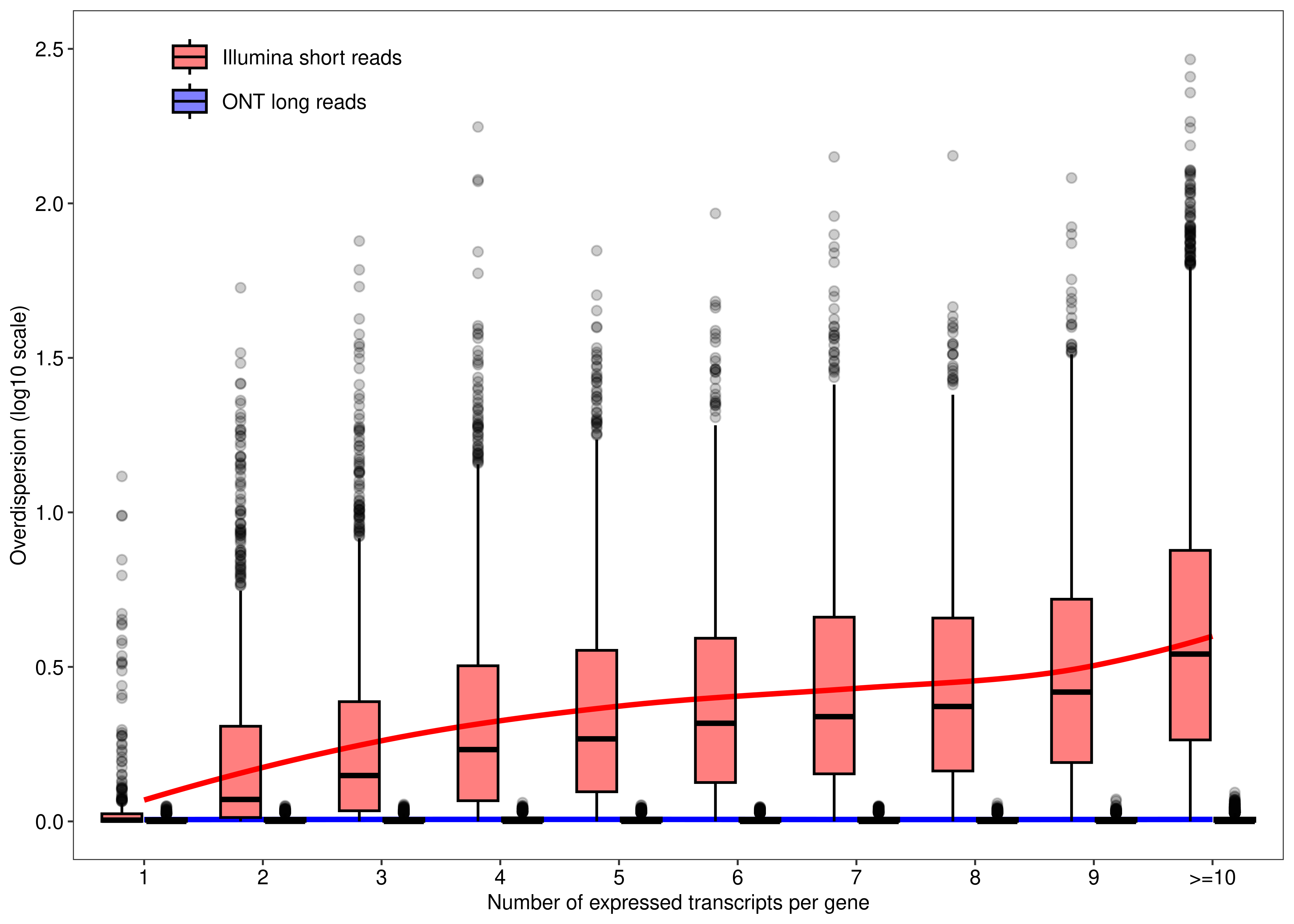

Past versions of casestudy_res_overdispersion-1.png

Version	Author	Date
1839ef1	Pedro Baldoni	2023-02-23

agg_png(filename = file.path(path.misc,"figure1.png"),
        width = 5,height = 5,units = 'in',res = 300)
plot.mao

`geom_smooth()` using formula = 'y ~ x'

dev.off()

png 
  2 

Comparison of transcript-level and gene-level results using paired-end read data

Then, we generate Figure 6 of the main paper below. First we generate panel (a).

# plotMDS returns invisible(), we need to manually export the plot (code from limma::plotMDS.MDS)
foo.mds <- function(x,fontsize = 8){
  obj.mds <- plotMDS(x,col = x$samples$Color,main = NULL)
  par(mar = c(5, 4, 2, 2))
  labels <- colnames(obj.mds$distance.matrix.squared)
  StringRadius <- 0.15 * 1 * nchar(labels)
  left.x <- obj.mds$x - StringRadius
  right.x <- obj.mds$x + StringRadius
  Perc <- round(obj.mds$var.explained * 100)
  xlab <- paste(obj.mds$axislabel, 1)
  ylab <- paste(obj.mds$axislabel, 2)
  xlab <- paste0(xlab, " (", Perc[1], "%)")
  ylab <- paste0(ylab, " (", Perc[2], "%)")
  
  plot(c(-3.5, 3.5), c(-1, 1.5),
       type = "n",xlab = xlab,ylab = ylab,
       cex.lab = fontsize/12,
       cex.axis = fontsize/12)
  text(obj.mds$x, obj.mds$y, labels = labels, cex = fontsize/12,col = x$samples$Color)
}

plot.mds <- wrap_elements(full = ~foo.mds(dte.short.paired.edger.scaled.filtr))

plot.mds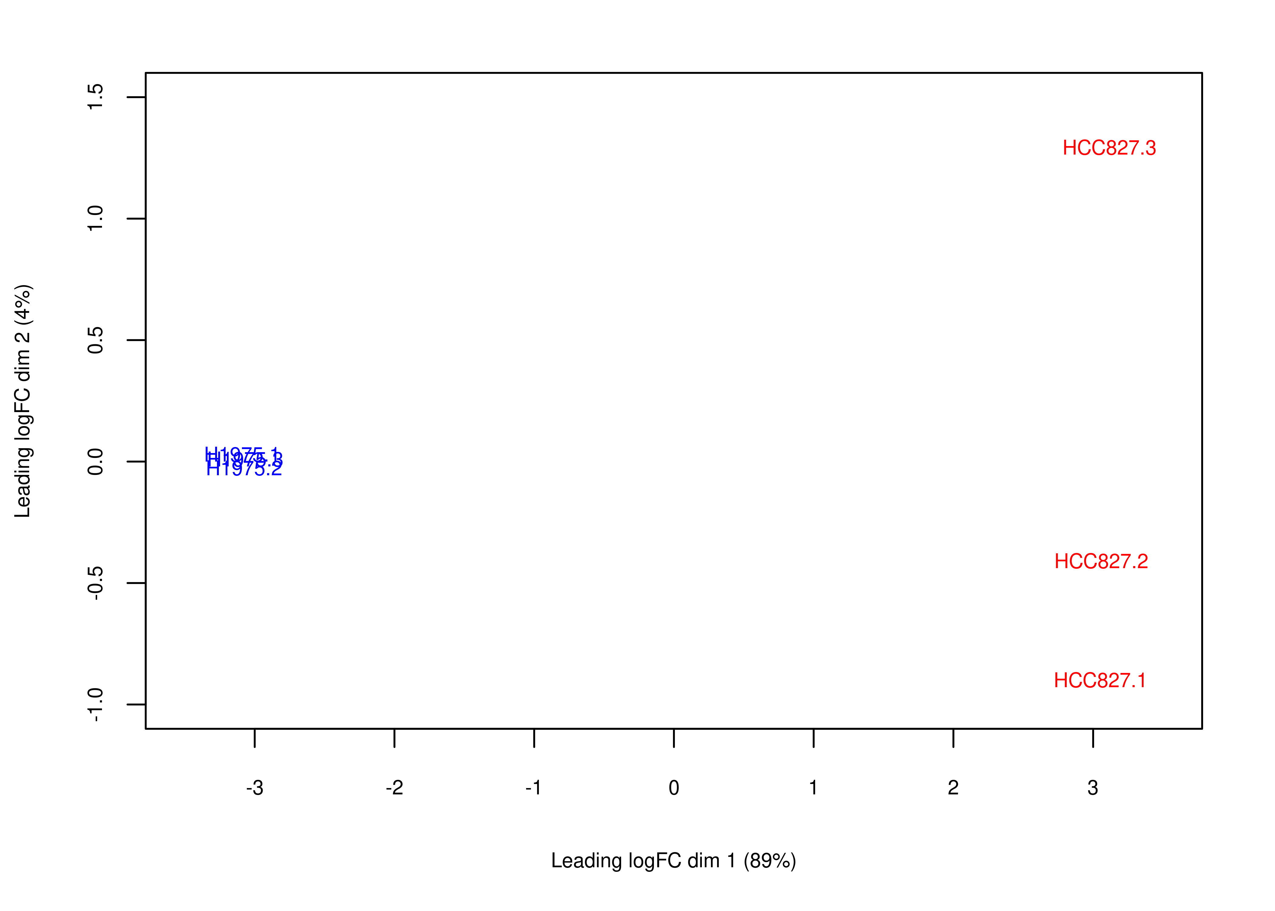

Past versions of casestudy_res_txgene_mds-1.png

Version	Author	Date
1839ef1	Pedro Baldoni	2023-02-23

Next, we generate panel (b).

# plotMD does not return invisible(), so we just use wrap_elements
foo.md <- function(x,fontsize = 8){
  par(mar = c(5, 4, 2, 2))
  plotMD(x,
         main = NULL,cex = 0.5,legend = FALSE,
         cex.lab = fontsize/12,
         cex.axis = fontsize/12)
  legend('topright',
         legend = c('NotSig','Up','Down'),
         pch = rep(16,3),
         col = c('black','red','blue'),
         cex = fontsize/12,
         pt.cex = c(0.3,0.5,0.5))
}
plot.md <-
  wrap_elements(full = ~foo.md(qlf.short.paired.edger.scaled))

plot.md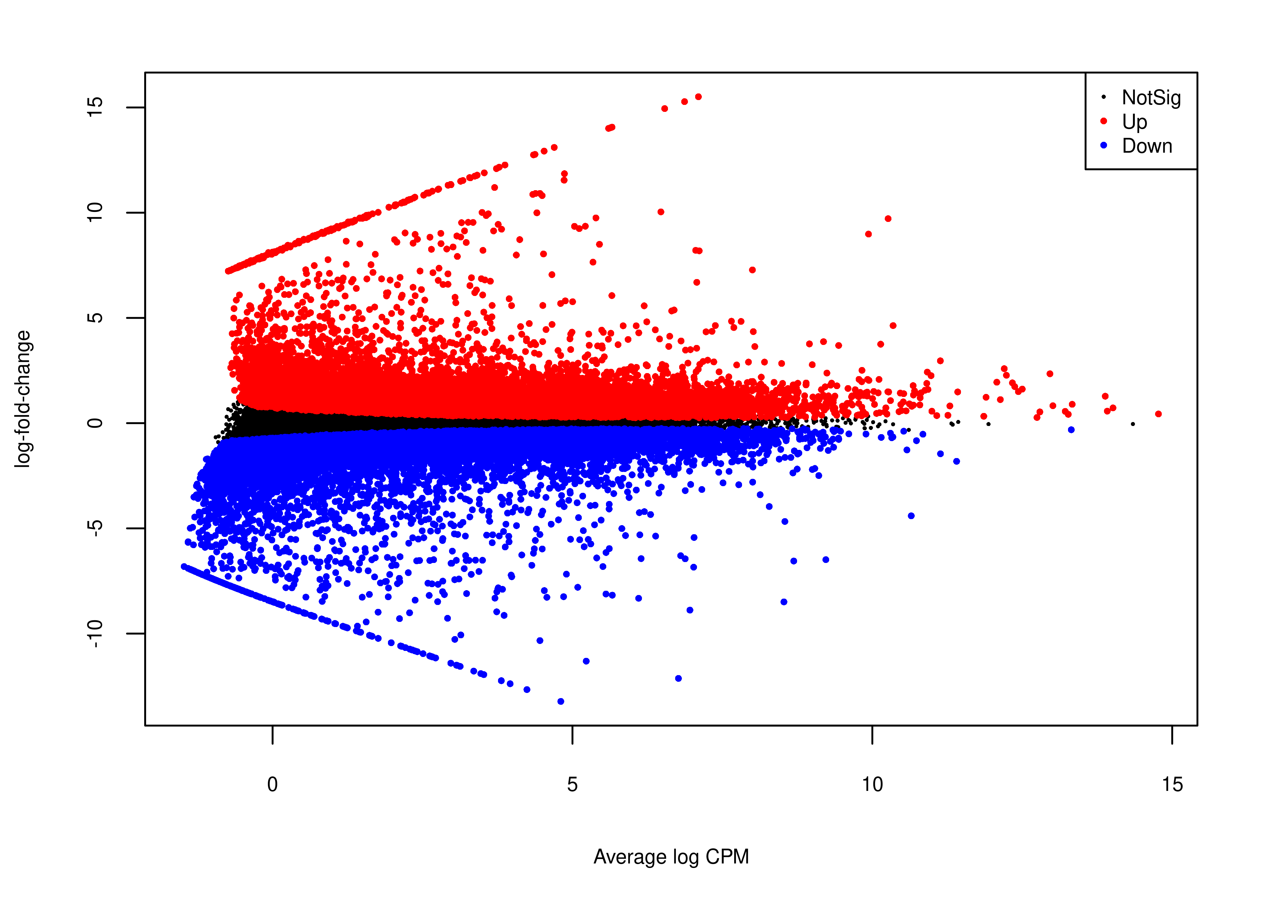

Past versions of casestudy_res_txgene_md-1.png

Version	Author	Date
1839ef1	Pedro Baldoni	2023-02-23

Panel (c) is created below.

foo.lolipop <- 
  function(symbols,gene.table,transcript.table, fontsize = 8,
           legend = c(0.9,0.9),
           colornames = c('NotSig' = 'black','Up' = 'red','Down' = 'blue')){
    
    ls.loli <- lapply(symbols,function(x){
      df.loli <-
        rbind(as.data.table(transcript.table$table[transcript.table$table$GeneSymbol == x,c('TranscriptSymbol','FDR','logFC')]),
              as.data.table(gene.table$table[gene.table$table$GeneName == x,c("FDR","logFC")]),fill = TRUE)
      df.loli[is.na(df.loli)] <- x
      df.loli$Color <- ifelse(df.loli$FDR > 0.05,'NotSig',ifelse(df.loli$logFC < 0,'Down','Up'))
      df.loli <- df.loli[order(df.loli$TranscriptSymbol),]
      df.loli$Gene <- x
      return(df.loli)
    })
    
    ls.loli <- do.call(rbind,ls.loli)
    
    ls.loli$Color <- factor(ls.loli$Color,levels = names(colornames))
    
    ggplot(data = ls.loli,aes(x = TranscriptSymbol,xend = TranscriptSymbol,yend = 0,y = logFC)) +
      facet_wrap('Gene',nrow = 1,scales = 'free_x') +
      geom_segment(color = 'black') +
      geom_point(size = 2,aes(color = Color)) +
      geom_hline(yintercept = 0) +
      geom_vline(xintercept = 1.5,linetype = 'dashed',color = 'gray') +
      scale_color_manual(values = colornames) +
      labs(x = NULL) +
      theme_bw(base_size = fontsize,base_family = 'sans') +
      theme(panel.grid = element_blank(),
            strip.background = element_blank(),
            strip.text = element_text(face = 'bold'),
            axis.text = element_text(colour = 'black',size = fontsize),
            legend.position = legend,
            axis.text.x = element_text(angle = 90, vjust = 0.5, hjust=1),
            legend.title = element_blank(),
            legend.text = element_text(colour = 'black',size = fontsize),
            legend.background=element_rect(fill = alpha("white", 0))) +
      guides(colour = guide_legend(keywidth=0.1,
                                   keyheight=0.1,
                                   default.unit="inch",
                                   override.aes = list(size = 0.75)))
  }

plot.lolipop <- wrap_elements(foo.lolipop(symbols = c('EGLN3','RAF1','MET','AKT1','BCL2L1'),
                                          gene.table = out.gene,
                                          transcript.table = out.short.paired.edger.scaled,legend = c(0.95,0.875)))
plot.lolipop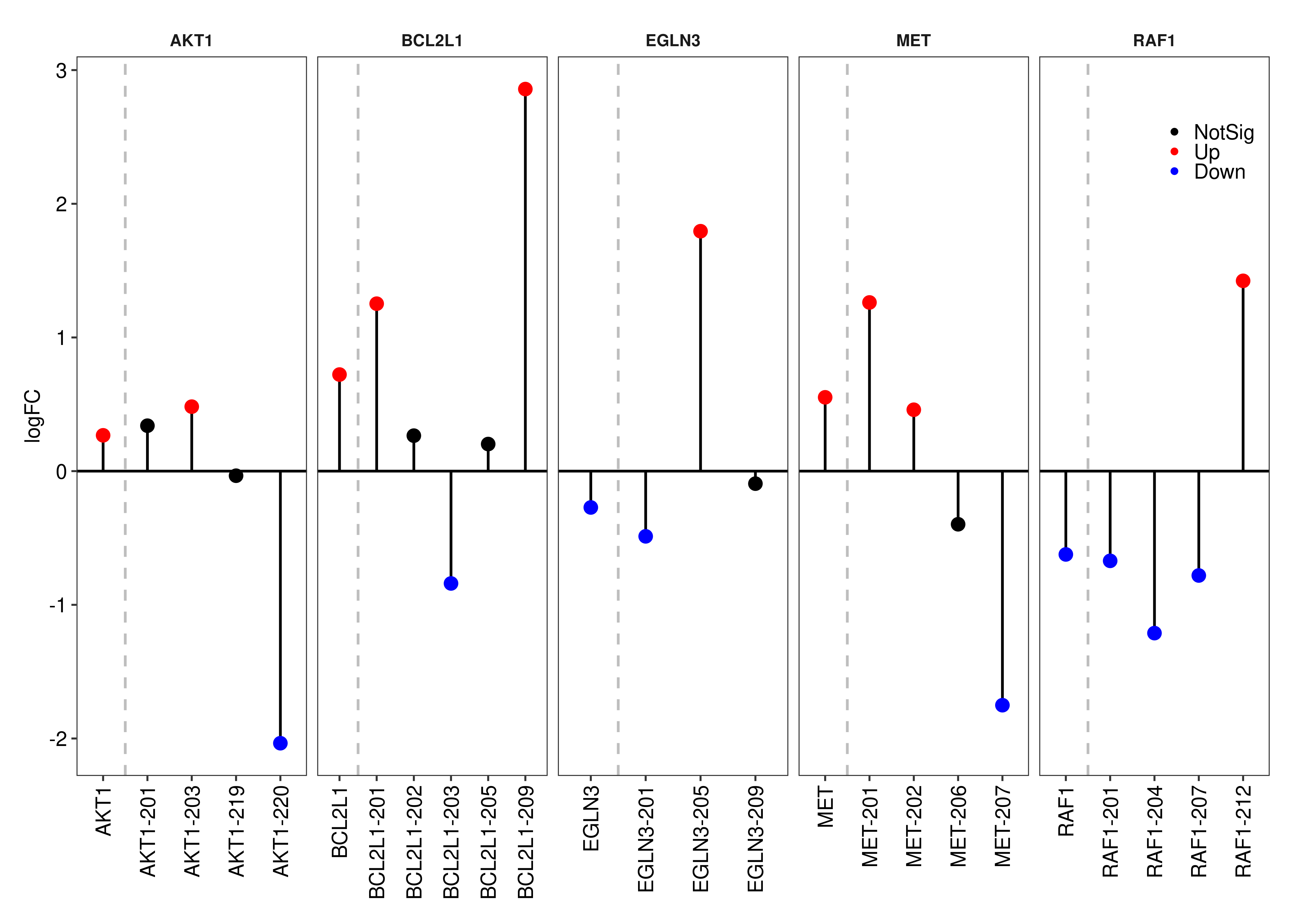

Past versions of casestudy_res_txgene_loliplot-1.png

Version	Author	Date
1839ef1	Pedro Baldoni	2023-02-23

Finally, we create panel (d). We use that package ComplexHeatmap Gu, Eils, and Schlesner (2016) to create the heatmap plot.

cpm.scaled <- cpm(dte.short.paired.edger.scaled.filtr,log = TRUE)
cpm.scaled <- t(scale(t(cpm.scaled)))

## Here I want to check non-significant genes associated with cancer pathways that have at least 1 DE transcript

df.tx.gene <- out.short.paired.edger.scaled$table
df.tx.gene$FDR.Gene <- 
  out.gene$table$FDR[match(df.tx.gene$GeneID,rownames(out.gene$table))]
interestGenes.ns <- 
  unique(df.tx.gene[df.tx.gene$FDR.Gene > 0.05 & 
                      df.tx.gene$FDR < 0.05 & 
                      df.tx.gene$GeneOfInterest == TRUE,"EntrezID"])

# Number of non-significant genes for which at least one of their transcripts is DE
length(interestGenes.ns)

[1] 841

# Running KEGG analysis
GK <- getGeneKEGGLinks(species.KEGG = "hsa")

interestGenes.ns.cancer <-
  interestGenes.ns[interestGenes.ns %in% 
                     GK$GeneID[GK$PathwayID %in% c('path:hsa05223','path:hsa05200')]]

# Number of non-significant genes for which at least one of their transcripts is DE
length(interestGenes.ns.cancer)

[1] 24

df.tx.gene.cancer <-
  df.tx.gene[df.tx.gene$EntrezID %in% interestGenes.ns.cancer,]

df.tx.gene.cancer <-
  df.tx.gene.cancer[df.tx.gene.cancer$FDR < 0.05,]

cpm.scaled.cancer <- cpm.scaled[rownames(df.tx.gene.cancer),]
rownames(cpm.scaled.cancer) <- 
  dte.short.paired.edger.scaled.filtr$genes$TranscriptSymbol[match(rownames(cpm.scaled.cancer),rownames(dte.short.paired.edger.scaled.filtr))]

foo.heat <- function(x,cluster_rows = TRUE, fontsize = 8,...){
  Heatmap(matrix = x,
          heatmap_legend_param = list(title = 'Expression',
                                      title_position = 'topcenter',
                                      direction = "horizontal",
                                      at = seq(-3,3,1),
                                      title_position = 'topcenter',
                                      title_gp = gpar(fontsize = fontsize),
                                      labels_gp = gpar(fontsize = fontsize)),
          cluster_rows = cluster_rows,
          row_names_gp = gpar(fontsize = fontsize),
          column_names_gp = gpar(fontsize = fontsize),
          col = c("blue", "white", "red"),...) %>%
    draw(heatmap_legend_side = "top")
}

plot.heat.cancer <-
  wrap_elements(grid.grabExpr(draw(foo.heat(t(cpm.scaled.cancer)))))

plot.heat.cancer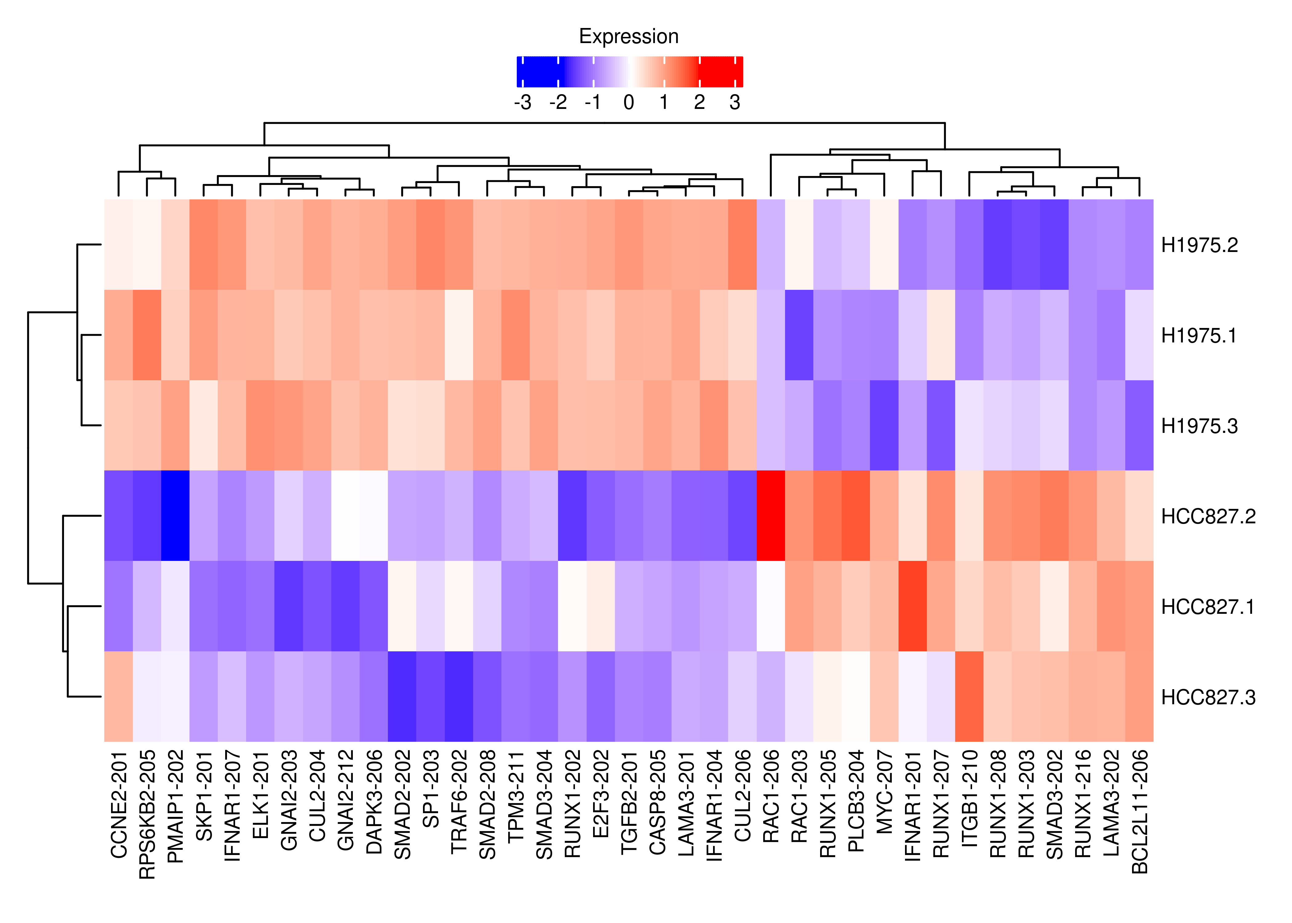

Past versions of casestudy_res_txgene_heat-1.png

Version	Author	Date
afee716	Pedro Baldoni	2023-02-25

Finally, we put all these plots together with the package patchwork Pedersen (2022).

plot.design <- c(area(1, 1),area(1,2),area(2,1,2,2),area(3,1,3,2))

fig.panel <- wrap_plots(A = plot.mds,
                        B = plot.md,
                        C = plot.lolipop,
                        D = plot.heat.cancer,
                        design = plot.design,
                        heights = c(0.35,0.25,0.4)) +
  plot_annotation(tag_levels = 'a')

fig.panel <- fig.panel &
  theme(plot.tag = element_text(size = 8))

agg_png(filename = file.path(path.misc,"figure6.png"),
        width = 10,height = 12,units = 'in',res = 300)
fig.panel
dev.off()

png 
  2 

For the genes presented in panel (b), below we present the results from our DE analysis at the gene-level.

tb.gene <- 
  out.gene$table[out.gene$table$GeneName %in% c('EGLN3','RAF1','MET','AKT1','BCL2L1'),]

tb.gene$EnsemblID <- rownames(tb.gene)
tb.gene <- data.frame(tb.gene[,c('EnsemblID','GeneName','EntrezID','GeneType',
                                 'logFC','logCPM','F','PValue','FDR')],row.names = NULL)
setnames(tb.gene,
         old = c('EnsemblID','GeneName','EntrezID','GeneType'),
         new = c('Ensembl ID','Symbol','Entrez ID','Biotype'))

tb.gene$Biotype <- gsub("_"," ",tb.gene$Biotype)

tb.gene$logFC <- formatC(round(tb.gene$logFC,3),digits = 3,format = 'f')
tb.gene$logCPM <- formatC(round(tb.gene$logCPM,3),digits = 3,format = 'f')
tb.gene$`F` <- formatC(round(tb.gene$`F`,3),digits = 3,format = 'f')
tb.gene$PValue <- formatC(tb.gene$PValue,digits = 3,format = 'e')
tb.gene$FDR <- formatC(tb.gene$FDR,digits = 3,format = 'e')

tb.gene$Biotype <- NULL

cap.kb.gene <- 
  paste('edgeR results from a DE analysis at the gene-level for',
        'a set of cancer-related genes comparing cell lines H1975 and HCC827.',
        'Data from the paired-end RNA-seq experiment of the the human cell lines (GSE172421).',
        'Such genes have at least one its transcripts differentially expressed between cell lines',
        '(nominal FDR 0.05 at the transcript-level).')

kb.gene <-
  kbl(tb.gene,
      escape = FALSE,
      format = 'latex',
      booktabs = TRUE,
      caption = cap.kb.gene,
      align = 'llcccccc') %>%
  kable_styling(font_size = 10)
save_kable(kb.gene,file = file.path(path.misc,"supptable_gene.tex"))

tb.gene

          Ensembl ID Symbol Entrez ID  logFC logCPM      F    PValue       FDR
1 ENSG00000132155.12   RAF1      5894 -0.623  5.942 39.959 1.465e-05 3.090e-05
2 ENSG00000171552.13 BCL2L1       598  0.723  8.187 28.776 8.277e-05 1.511e-04
3 ENSG00000105976.15    MET      4233  0.552  9.092 24.635 1.773e-04 3.064e-04
4 ENSG00000129521.14  EGLN3    112399 -0.272  5.197  7.648 1.458e-02 1.923e-02
5 ENSG00000142208.16   AKT1       207  0.268  7.431  5.828 2.922e-02 3.714e-02

Another set of interesting genes are those that are statistically significant and have trnascripts being DE in a different direction between conditions. Let’s take a look at those.

df.tx.gene$logFC.Gene <- 
  out.gene$table$logFC[match(df.tx.gene$GeneID,rownames(out.gene$table))]

interestGenes.s <-
  unique(df.tx.gene[df.tx.gene$FDR.Gene < 0.05 &
                      df.tx.gene$FDR < 0.05 &
                      sign(df.tx.gene$logFC) != sign(df.tx.gene$logFC.Gene) &
                      !is.na(df.tx.gene$logFC.Gene) &
                      df.tx.gene$GeneOfInterest == TRUE,"EntrezID"])

interestGenes.s.cancer <-
  interestGenes.s[interestGenes.s %in% GK$GeneID[GK$PathwayID %in% c('path:hsa05223','path:hsa05200')]]

# Number of significant genes (and cancer-related genes) for which at least one of their transcripts is DE and going in the opposite direction
length(interestGenes.s)

[1] 403

length(interestGenes.s.cancer)

[1] 12

# Creating heatmat for such genes and their DE transcripts

df.tx.gene.s <-
  df.tx.gene[df.tx.gene$EntrezID %in% interestGenes.s,]

df.tx.gene.s.cancer <-
  df.tx.gene[df.tx.gene$EntrezID %in% interestGenes.s.cancer,]

df.tx.gene.s <-
  df.tx.gene.s[df.tx.gene.s$FDR < 0.05 & 
                 sign(df.tx.gene.s$logFC) != sign(df.tx.gene.s$logFC.Gene),]

df.tx.gene.s.cancer <-
  df.tx.gene.s.cancer[df.tx.gene.s.cancer$FDR < 0.05 & 
                        sign(df.tx.gene.s.cancer$logFC) != sign(df.tx.gene.s.cancer$logFC.Gene),]

cpm.scaled.s.cancer <- cpm.scaled[rownames(df.tx.gene.s.cancer),]
rownames(cpm.scaled.s.cancer) <- dte.short.paired.edger.scaled.filtr$genes$TranscriptSymbol[match(rownames(cpm.scaled.s.cancer),rownames(dte.short.paired.edger.scaled.filtr))]

cpm.scaled.s <- cpm.scaled[rownames(df.tx.gene.s),]
rownames(cpm.scaled.s) <- dte.short.paired.edger.scaled.filtr$genes$TranscriptSymbol[match(rownames(cpm.scaled.s),rownames(dte.short.paired.edger.scaled.filtr))]

plot.heat.s <-
  wrap_elements(grid.grabExpr(draw(foo.heat(cpm.scaled.s,show_row_names = FALSE))))

plot.heat.s.cancer <-
  wrap_elements(grid.grabExpr(draw(foo.heat(cpm.scaled.s.cancer))))

plot.heat.s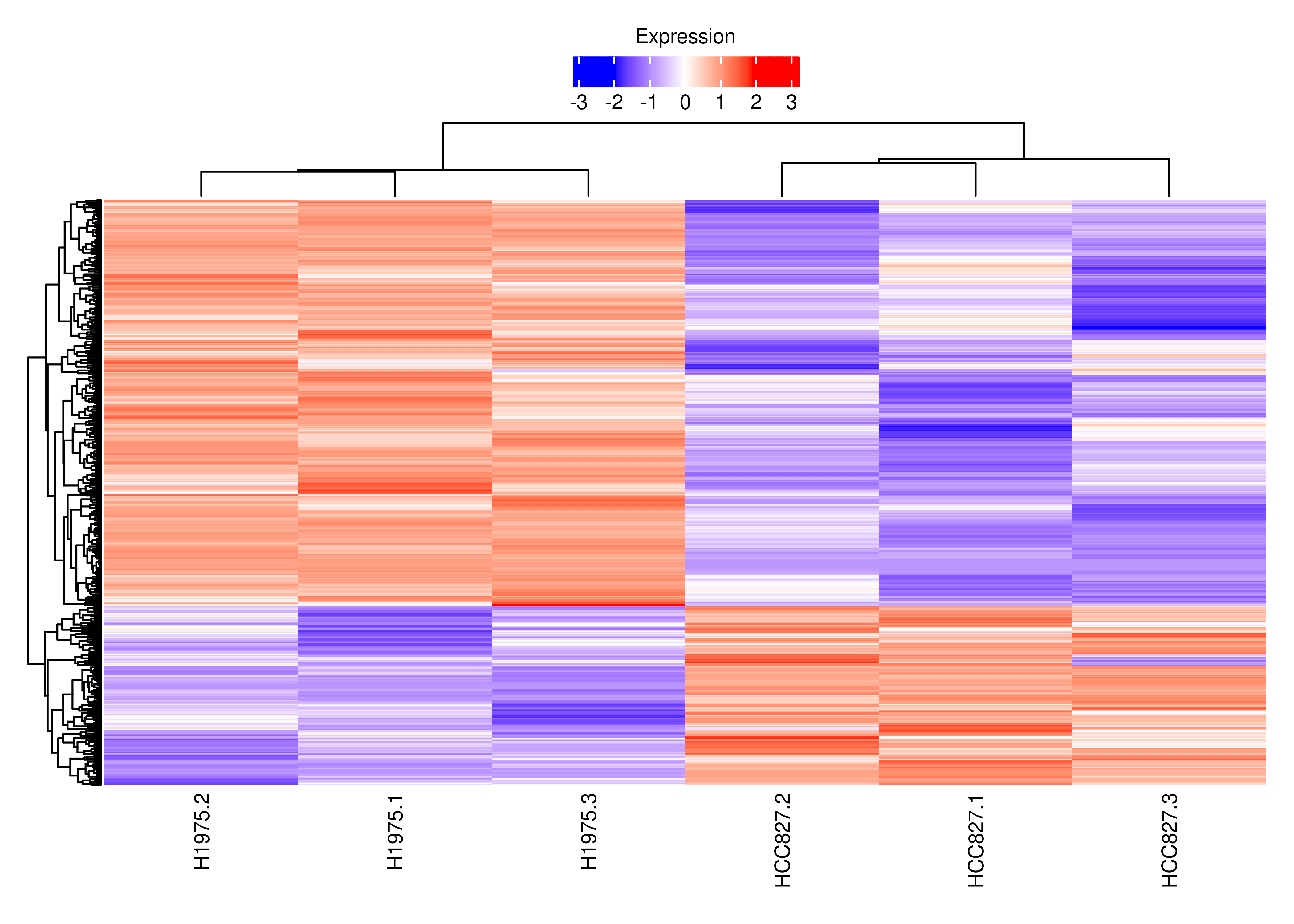

Past versions of casestudy_res_txgene_switch-1.png

Version	Author	Date
280d68a	Pedro Baldoni	2023-02-25

plot.heat.s.cancer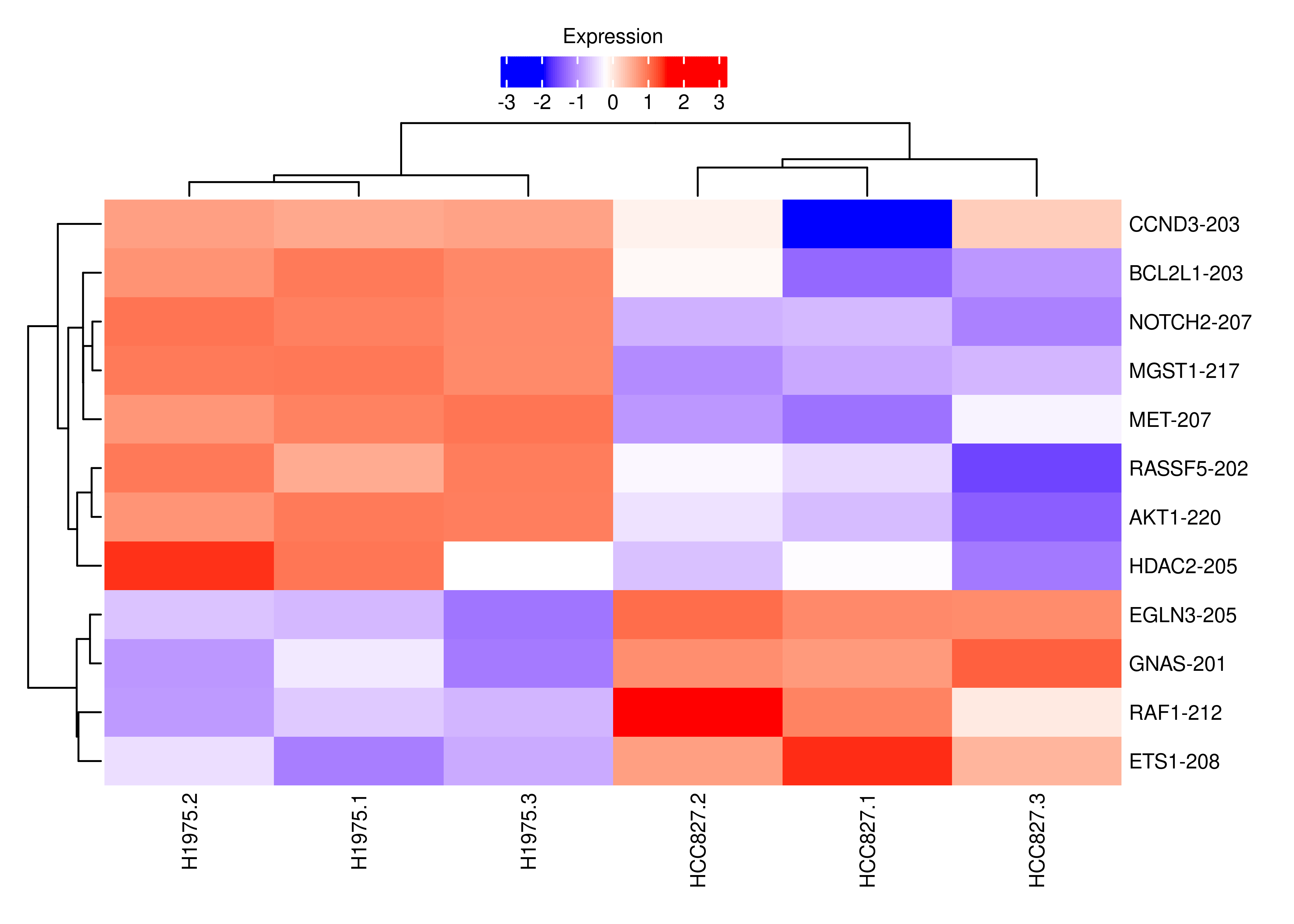

Past versions of casestudy_res_txgene_switch-2.png

Version	Author	Date
280d68a	Pedro Baldoni	2023-02-25

We can also compare the distribution of the overdispersion estimates between gene- and transcript-level analyses.

df.output.gene <-
  as.data.table(dge$genes[,c('GeneName','EntrezID','GeneType','Overdispersion')])
setnames(df.output.gene,
         old = c('GeneName','EntrezID','GeneType','Overdispersion'),
         new = c('Symbol','EntrezID','Type','Overdispersion'))
df.output.gene[,Level := 'Gene']
df.output.gene$EnsemblID <- rownames(dge)

## Transcript-level
df.output.tx <- 
  data.table(Symbol = dte.short.paired.edger.scaled$genes$TranscriptSymbol,
             EntrezID = dte.short.paired.edger.scaled$genes$EntrezID,
             Type = dte.short.paired.edger.scaled$genes$GeneType,
             Overdispersion = catch.short.paired$annotation$Overdispersion,
             Level = 'Transcript',
             EnsemblID = rownames(dte.short.paired.edger.scaled$genes))


df.output.gene.tx <- rbindlist(list(df.output.gene,df.output.tx))

fig.mao.gene.tx <- ggplot(df.output.gene.tx,aes(x = log10(Overdispersion),y = Level,fill = Level)) +
  geom_boxplot(outlier.alpha = 0.25,fill = "#bebebe",col = 'black') +
  labs(y = NULL,x = 'Mapping ambiguity overdispersion (log10 scale)') +
  theme_bw(base_size = 8,base_family = 'sans') +
  theme(legend.position = 'none',
        panel.grid = element_blank(),
        axis.text = element_text(colour = 'black',size = 8))

agg_png(filename = file.path(path.misc,"suppfigure_overdispersion.png"),
        width = 7.5,height = 5,units = 'in',res = 300)
fig.mao.gene.tx
dev.off()

png 
  2 

fig.mao.gene.tx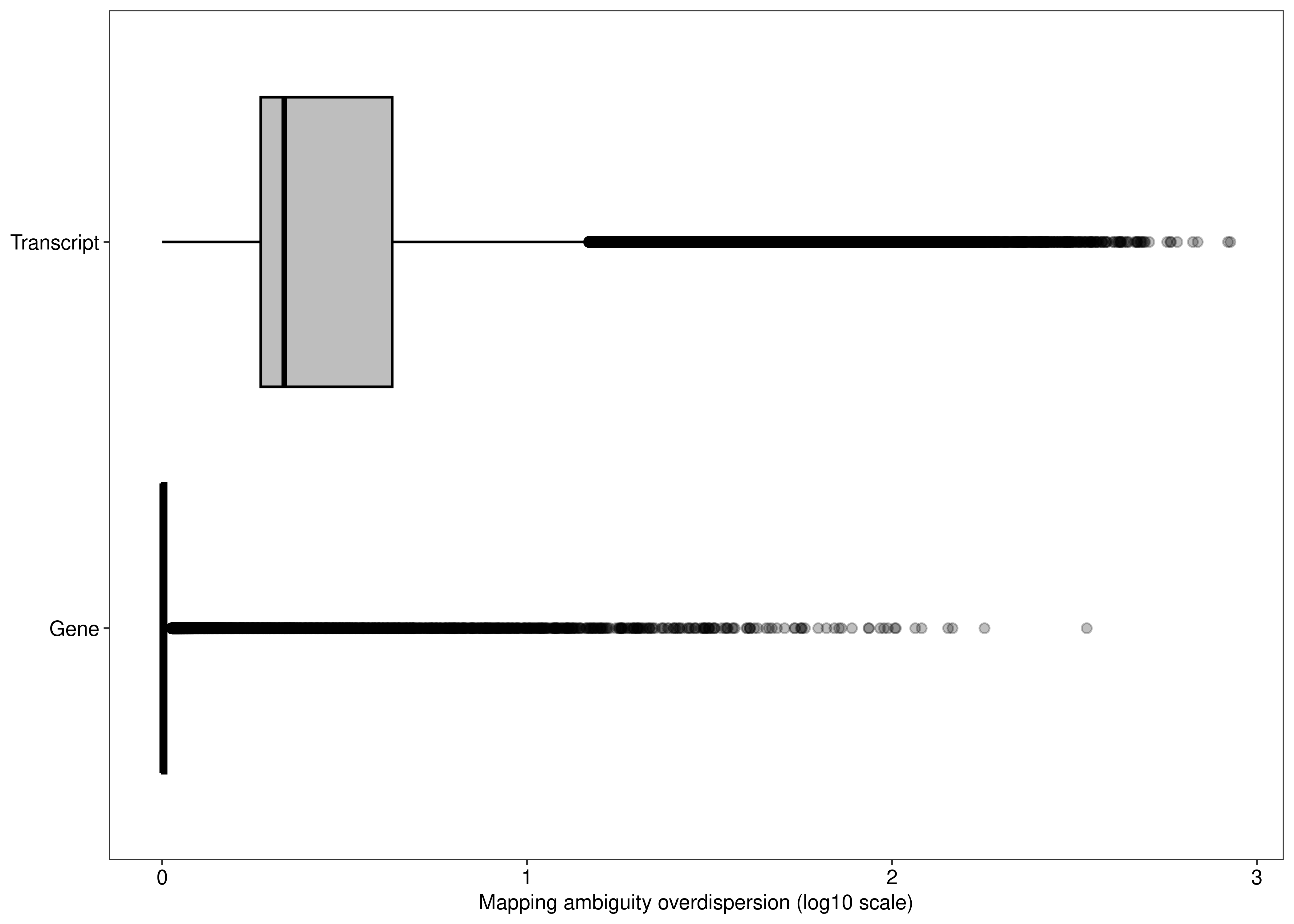

Past versions of casestudy_res_txgene_overdispersion-1.png

Version	Author	Date
afee716	Pedro Baldoni	2023-02-25

Below we have a table of the top genes with highest mapping ambiguity estimated overdispersion. Most of such genes do not have an associated Entrez ID.

df.output.gene.top <- 
  df.output.gene[order(-Overdispersion),][1:100,c('EnsemblID','Symbol','Type','EntrezID','Overdispersion')]
df.output.gene.top$Type <- gsub("_"," ",df.output.gene.top$Type)
df.output.gene.top$EntrezID[is.na(df.output.gene.top$EntrezID)] <- "-"

cap.mao <- paste("Top 100 genes with largest mapping ambiguity overdispersion.",
                 "Data from the RNA-seq experiment of the human cell lines",
                 "generated with paired-end reads (GSE172421).")

kb.output.gene.top <- 
  kbl(df.output.gene.top,
      longtable = TRUE,
      escape = FALSE,
      format = 'latex',
      booktabs = TRUE,
      caption = cap.mao,
      digits = 2,
      align = c('lllcc'),
      col.names = c('Ensembl ID','Symbol','Entrez ID','Biotype','Overdispersion')) %>%
  kable_styling(latex_options = c("scale_down","repeat_header"),font_size = 10)

Warning in styling_latex_scale_down(out, table_info): Longtable cannot be
resized.

save_kable(kb.output.gene.top,file = file.path(path.misc,"supptable_overdispersion.tex"))

df.output.gene.top

              EnsemblID         Symbol                             Type
  1: ENSG00000205609.12         EIF3CL                   protein coding
  2:  ENSG00000278996.1     FP671120.5                           lncRNA
  3:  ENSG00000268861.7     AC008878.3                   protein coding
  4:  ENSG00000285238.2     AC006064.6                   protein coding
  5: ENSG00000015568.13          RGPD5                   protein coding
  6: ENSG00000178397.13        FAM220A                   protein coding
  7:  ENSG00000253797.2         UTP14C                   protein coding
  8:  ENSG00000277067.4     CU634019.2                           lncRNA
  9:  ENSG00000259040.5 BLOC1S5-TXNDC5                   protein coding
 10:  ENSG00000254692.1     AL136295.1                   protein coding
 11:  ENSG00000283782.2     AC116366.3                   protein coding
 12:  ENSG00000285447.1         ZNF883                   protein coding
 13:  ENSG00000279809.1     AC005538.2                              TEC
 14:  ENSG00000259132.1     AL132780.3                   protein coding
 15:  ENSG00000269547.1     AC011455.2                   protein coding
 16:  ENSG00000284057.1     AP001273.2                   protein coding
 17: ENSG00000154545.16         MAGED4                   protein coding
 18:  ENSG00000288534.1     AP001931.2                   protein coding
 19:  ENSG00000257411.2     AC034102.2                   protein coding
 20:  ENSG00000261771.5   DNAAF4-CCPG1                           lncRNA
 21:  ENSG00000256861.1     AC048338.1                   protein coding
 22:  ENSG00000260537.2     AC012184.2                   protein coding
 23:  ENSG00000202198.1     AL162581.1                         misc RNA
 24:  ENSG00000273590.4        SMIM11B                   protein coding
 25:  ENSG00000234289.6          H2BS1                   protein coding
 26:  ENSG00000268738.3          HSFX2                   protein coding
 27:  ENSG00000270276.2          H4C15                   protein coding
 28:  ENSG00000276077.4     CU633904.2                           lncRNA
 29:  ENSG00000286600.1     AC119427.2                           lncRNA
 30:  ENSG00000235655.3           H3P6             processed pseudogene
 31:  ENSG00000249624.9     AP000295.1                   protein coding
 32:  ENSG00000249590.7     AC004832.3                   protein coding
 33: ENSG00000132207.17          SLX1A                   protein coding
 34:  ENSG00000261915.6     AC026954.2                   protein coding
 35:  ENSG00000283239.1     AC019257.8                   protein coding
 36:  ENSG00000286075.1     AC009412.1                   protein coding
 37:  ENSG00000272921.1     AC005832.4                   protein coding
 38:  ENSG00000270181.3     BIVM-ERCC5                   protein coding
 39: ENSG00000183054.11          RGPD6                   protein coding
 40:  ENSG00000180658.4          OR2A4                   protein coding
 41:  ENSG00000249839.1     AC011330.1           unprocessed pseudogene
 42:  ENSG00000196826.7     AC008758.1                   protein coding
 43:  ENSG00000269900.3           RMRP                           lncRNA
 44:  ENSG00000270316.1    BORCS7-ASMT                   protein coding
 45:  ENSG00000130283.9           GDF1                   protein coding
 46:  ENSG00000260371.1     AC026464.3                   protein coding
 47:  ENSG00000285258.1          ATXN7                   protein coding
 48:  ENSG00000188223.9     AD000671.1                   protein coding
 49:  ENSG00000254673.1     AC110275.1                   protein coding
 50:  ENSG00000271672.1         DUXAP8 transcribed processed pseudogene
 51: ENSG00000167131.17        CCDC103                   protein coding
 52:  ENSG00000231259.5     AC125232.1           unprocessed pseudogene
 53:  ENSG00000256349.1     AP002748.5                   protein coding
 54: ENSG00000160201.11          U2AF1                   protein coding
 55:  ENSG00000234964.4        FABP5P7             processed pseudogene
 56:  ENSG00000284554.2     AL022318.4                   protein coding
 57:  ENSG00000258465.8     AL139011.2                   protein coding
 58: ENSG00000124208.16 TMEM189-UBE2V1                   protein coding
 59: ENSG00000184110.14          EIF3C                   protein coding
 60:  ENSG00000285901.1     AC008012.1                   protein coding
 61:  ENSG00000284989.1     AL451062.4                   protein coding
 62:  ENSG00000257315.2          ZBED6                   protein coding
 63:  ENSG00000285404.1       Z82190.2                   protein coding
 64:  ENSG00000287856.1     AL445524.2                   protein coding
 65: ENSG00000205670.11        SMIM11A                   protein coding
 66:  ENSG00000180581.7         SRP9P1             processed pseudogene
 67:  ENSG00000235288.3     AC099329.1                           lncRNA
 68:  ENSG00000262526.2     AC120057.2                   protein coding
 69:  ENSG00000285304.1       Z83844.3                   protein coding
 70:  ENSG00000224831.3       TMEM183B             processed pseudogene
 71:  ENSG00000285130.2     AL358113.1                   protein coding
 72:  ENSG00000214076.3        CPSF1P1 transcribed processed pseudogene
 73:  ENSG00000267645.5     AC105052.3                   protein coding
 74:  ENSG00000279423.1     AL445363.3                              TEC
 75:  ENSG00000268173.3     AC007192.1                   protein coding
 76:  ENSG00000280987.4          MATR3                   protein coding
 77:  ENSG00000285585.1     AC069444.2                   protein coding
 78:  ENSG00000281453.1      TGFB2-OT1                           lncRNA
 79:  ENSG00000235884.4      LINC00941                           lncRNA
 80:  ENSG00000271153.1      RPL23AP88             processed pseudogene
 81:  ENSG00000285920.2     AC087721.2                   protein coding
 82:  ENSG00000285053.1           TBCE                   protein coding
 83:  ENSG00000277125.1    AC211476.10           unprocessed pseudogene
 84:  ENSG00000283201.1     AC092329.3                   protein coding
 85:  ENSG00000257767.3     AC002996.1                   protein coding
 86:  ENSG00000285953.1     AC000120.4                   protein coding
 87:  ENSG00000270066.3     AL356488.2                           lncRNA
 88:  ENSG00000285565.1     AL671762.1                           lncRNA
 89:  ENSG00000270882.2          H4C14                   protein coding
 90:  ENSG00000198406.7         BZW1P2             processed pseudogene
 91:  ENSG00000269711.1     AC008763.3                   protein coding
 92:  ENSG00000286098.1     AC008770.4                   protein coding
 93:  ENSG00000283765.1     AC131160.1                   protein coding
 94:  ENSG00000264545.2     AL359922.1                   protein coding
 95:  ENSG00000288380.1     AC118281.1                   protein coding
 96: ENSG00000243708.10        PLA2G4B                   protein coding
 97:  ENSG00000232882.1        PHKA1P1             processed pseudogene
 98: ENSG00000163635.18          ATXN7                   protein coding
 99:  ENSG00000264668.2     AC138696.1                   protein coding
100: ENSG00000172780.16          RAB43                   protein coding
              EnsemblID         Symbol                             Type
      EntrezID Overdispersion
  1:    728689      341.55329
  2:         -      179.20069
  3:     23370      146.41457
  4:         -      142.45960
  5:     84220      120.50852
  6:     84792      115.78457
  7:      9724      102.41948
  8: 102724843      101.81897
  9:         -       97.40022
 10:         -       95.06763
 11:         -       92.76017
 12:    169834       86.45160
 13:         -       86.20744
 14:         -       77.62727
 15:         -       72.68414
 16:         -       71.60434
 17:    728239       69.52741
 18:         -       66.12744
 19:         -       62.77753
 20:         -       57.69913
 21:         -       56.66263
 22:         -       56.46824
 23:         -       56.15088
 24: 102723553       54.19200
 25:     54145       54.01728
 26: 100130086       50.75873
 27:    554313       48.34551
 28: 102724951       46.84375
 29:         -       46.00233
 30:         -       45.17108
 31:         -       42.82163
 32:         -       41.94934
 33:    548593       40.81429
 34:         -       40.80824
 35:         -       40.72144
 36:         -       40.08434
 37:         -       39.92555
 38:         -       37.08285
 39:    729540       36.74529
 40:     79541       36.51568
 41:         -       35.48179
 42:         -       35.26890
 43:         -       35.17539
 44:         -       34.80449
 45:      2657       34.07745
 46:         -       32.72416
 47:      6314       32.57430
 48:         -       32.55255
 49:         -       32.18210
 50:         -       31.58082
 51:    388389       31.58059
 52:         -       31.44377
 53:         -       31.32582
 54:      7307       30.91959
 55:         -       30.72538
 56:         -       30.62995
 57:         -       30.62523
 58:    387522       30.39804
 59:      8663       30.31766
 60:         -       29.90434
 61:         -       29.06666
 62: 100381270       28.83286
 63:         -       28.79896
 64:         -       28.14299
 65:     54065       27.81531
 66:         -       27.74589
 67:         -       27.42346
 68:         -       26.60494
 69:         -       26.17273
 70:         -       26.16531
 71:         -       25.91874
 72:         -       25.53335
 73:         -       25.42465
 74:         -       25.18152
 75:         -       25.17870
 76:      9782       24.43611
 77:         -       24.25211
 78:         -       23.69302
 79:         -       23.51383
 80:         -       23.32973
 81:         -       22.44191
 82:      6905       22.12165
 83:         -       22.02204
 84:    440519       21.67864
 85:         -       21.65601
 86:         -       21.53951
 87:         -       21.32237
 88:         -       21.11837
 89:      8370       20.78220
 90:         -       20.66036
 91:         -       20.46554
 92:    284391       20.30157
 93:     55486       20.23441
 94:         -       20.11421
 95:         -       20.08538
 96: 100137049       20.06304
 97:         -       19.97567
 98:      6314       19.81824
 99:         -       19.63181
100:    339122       19.61291
      EntrezID Overdispersion

Comparison between analyses using paired- and single-end reads

Finally, we can compute how many transcripts are being called as DE using both paired- and single-end Illumina short reads. We add the transcript-level results from ONT long read data as a comparison.

tb.tx.genes <- dte.short.paired$genes

tb.tx.genes$FDR.SE <- 
  out.short.single.edger.scaled$table$FDR[match(rownames(tb.tx.genes),rownames(out.short.single.edger.scaled))]

tb.tx.genes$FDR.PE <- 
  out.short.paired.edger.scaled$table$FDR[match(rownames(tb.tx.genes),rownames(out.short.paired.edger.scaled))]

tb.tx.genes$FDR.LR <- out.long$table$FDR[match(rownames(tb.tx.genes),rownames(out.long))]

tb.tx.genes <- (tb.tx.genes[,c('FDR.SE','FDR.PE','FDR.LR')] < 0.05)*1L
tb.tx.genes[is.na(tb.tx.genes)] <- 0L

plot.venn <- 
  wrap_elements(full = ~ vennDiagram(tb.tx.genes[,c('FDR.SE','FDR.PE','FDR.LR')],
                                     names = c('Illumina\nsingle-end reads',
                                               'Illumina\npaired-end reads',
                                               'ONT\nlong reads'),
                                     circle.col = c('salmon','red','blue'),cex = c(12,10,8)/12))

agg_png(filename = file.path(path.misc,"suppfigure_venn.png"),
        width = 6,height = 6,units = 'in',res = 300)
plot.venn
dev.off()

png 
  2 

plot.venn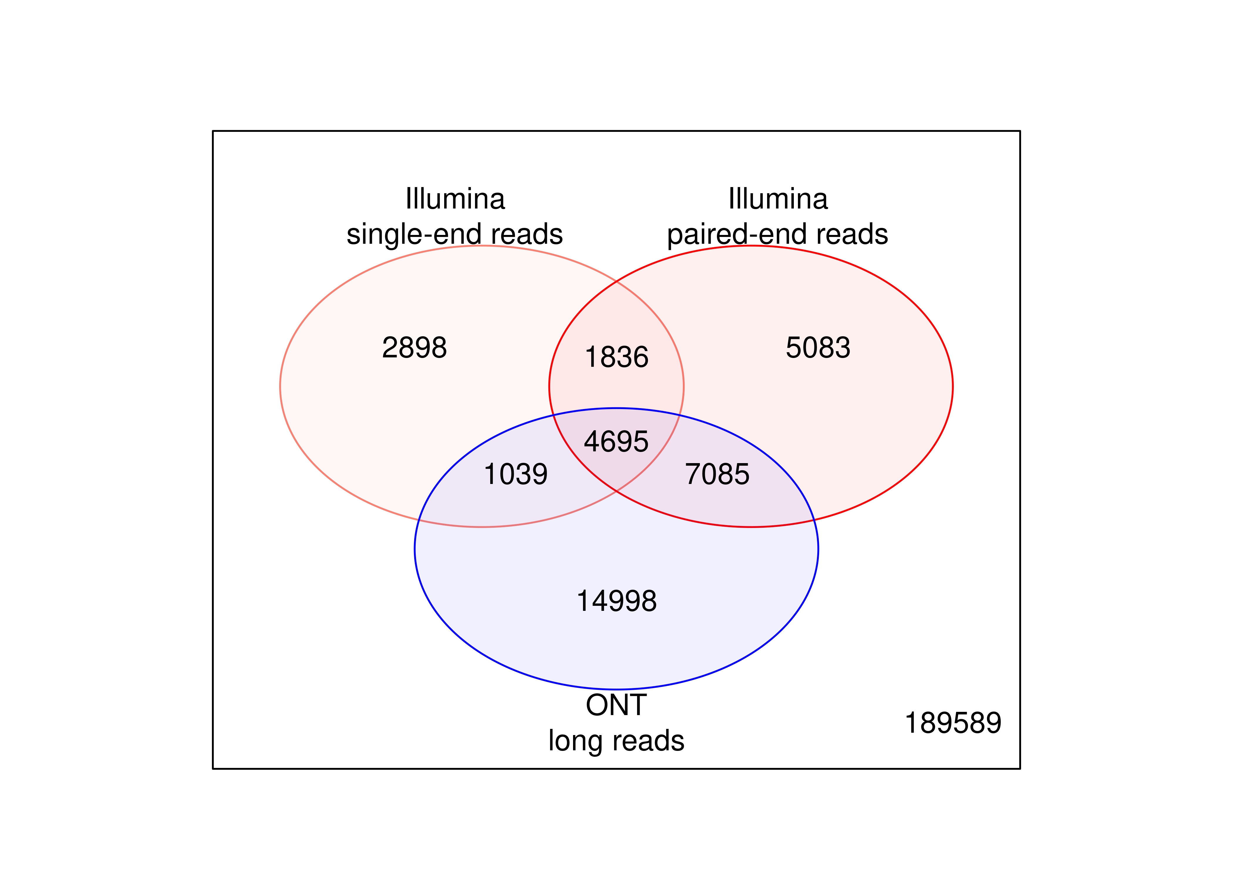

Past versions of casestudy_res_sepe_venn-1.png

Version	Author	Date
afee716	Pedro Baldoni	2023-02-25

And the MA plot highlighting DE transcripts called with single-end Illumina short reads is presented below.

plot.md.se <-
  wrap_elements(full = ~foo.md(qlf.short.single.edger.scaled))

agg_png(filename = file.path(path.misc,"suppfigure_maplot.png"),
        width = 6,height = 6,units = 'in',res = 300)
plot.md.se
dev.off()

png 
  2 

plot.md.se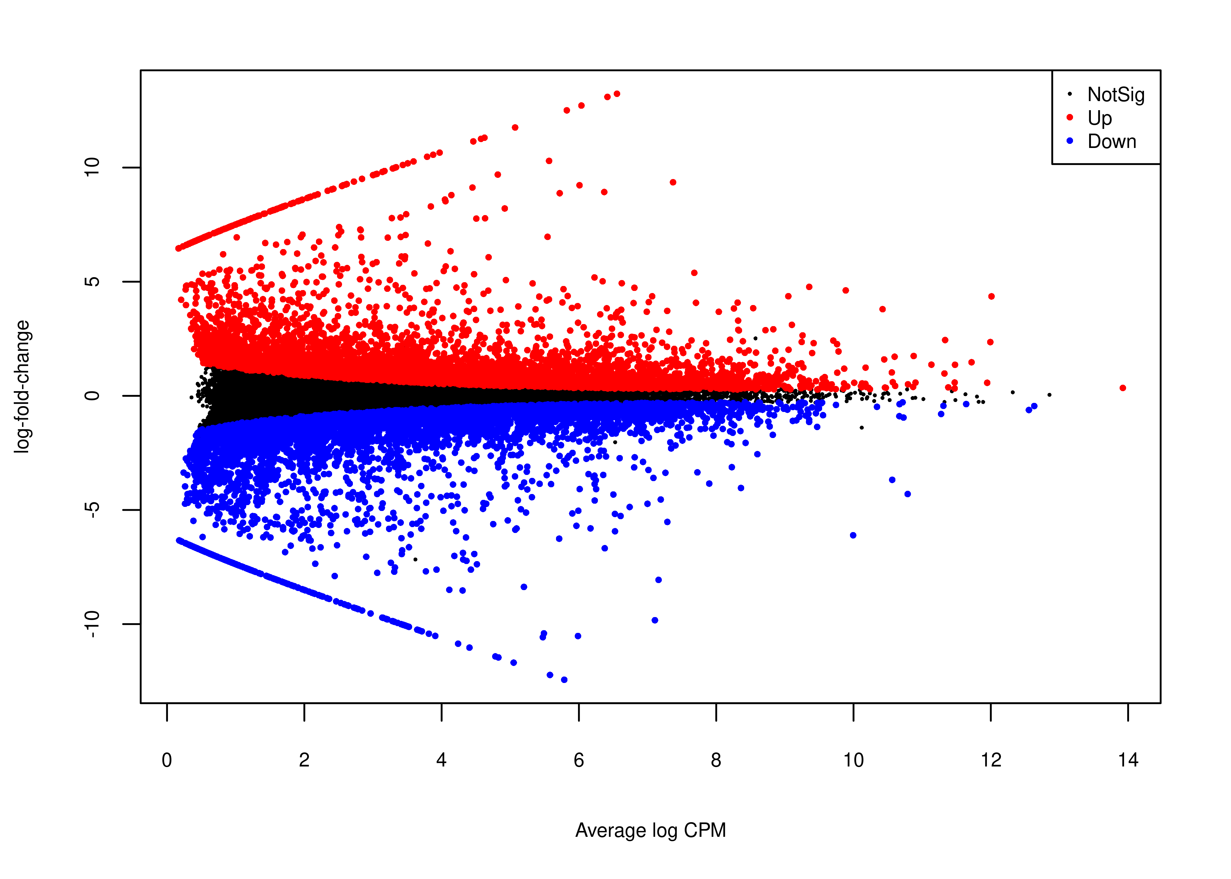

Past versions of casestudy_res_sepe_ma-1.png

Version	Author	Date
afee716	Pedro Baldoni	2023-02-25

Gu, Zuguang, Roland Eils, and Matthias Schlesner. 2016. “Complex Heatmaps Reveal Patterns and Correlations in Multidimensional Genomic Data.” Bioinformatics 32 (18): 2847–49.

Love, Michael I, Charlotte Soneson, Peter F Hickey, Lisa K Johnson, N Tessa Pierce, Lori Shepherd, Martin Morgan, and Rob Patro. 2020. “Tximeta: Reference Sequence Checksums for Provenance Identification in RNA-Seq.” PLoS Computational Biology 16 (2): e1007664. https://doi.org/10.1371/journal.pcbi.1007664.

Pedersen, Thomas Lin. 2022. Patchwork: The Composer of Plots.

Qu, Shuang, Zichen Jiao, Geng Lu, Bing Yao, Ting Wang, Weiwei Rong, Jiahan Xu, et al. 2021. “PD-L1 lncRNA Splice Isoform Promotes Lung Adenocarcinoma Progression via Enhancing c-Myc Activity.” Genome Biology 22 (1): 1–24.

Yang, In Seok, and Sangwoo Kim. 2018. “Isoform Specific Gene Expression Analysis of KRAS in the Prognosis of Lung Adenocarcinoma Patients.” BMC Bioinformatics 19 (1): 1–10.

Session information

sessionInfo()

R version 4.2.1 (2022-06-23)
Platform: x86_64-pc-linux-gnu (64-bit)
Running under: CentOS Linux 7 (Core)

Matrix products: default
BLAS:   /stornext/System/data/apps/R/R-4.2.1/lib64/R/lib/libRblas.so
LAPACK: /stornext/System/data/apps/R/R-4.2.1/lib64/R/lib/libRlapack.so

locale:
 [1] LC_CTYPE=en_US.UTF-8       LC_NUMERIC=C              
 [3] LC_TIME=en_US.UTF-8        LC_COLLATE=en_US.UTF-8    
 [5] LC_MONETARY=en_US.UTF-8    LC_MESSAGES=en_US.UTF-8   
 [7] LC_PAPER=en_US.UTF-8       LC_NAME=C                 
 [9] LC_ADDRESS=C               LC_TELEPHONE=C            
[11] LC_MEASUREMENT=en_US.UTF-8 LC_IDENTIFICATION=C       

attached base packages:
[1] grid      stats4    stats     graphics  grDevices utils     datasets 
[8] methods   base     

other attached packages:
 [1] ensembldb_2.22.0            AnnotationFilter_1.22.0    
 [3] GenomicFeatures_1.50.4      AnnotationDbi_1.60.0       
 [5] kableExtra_1.3.4            magrittr_2.0.3             
 [7] ggplot2_3.4.1               ragg_1.2.5                 
 [9] tibble_3.1.8                ComplexHeatmap_2.14.0      
[11] patchwork_1.1.2             sleuth_0.30.0              
[13] fishpond_2.4.1              SummarizedExperiment_1.28.0
[15] Biobase_2.58.0              GenomicRanges_1.50.2       
[17] GenomeInfoDb_1.34.9         IRanges_2.32.0             
[19] S4Vectors_0.36.1            MatrixGenerics_1.10.0      
[21] matrixStats_0.63.0          tximeta_1.16.1             
[23] data.table_1.14.6           AnnotationHub_3.6.0        
[25] BiocFileCache_2.6.0         dbplyr_2.3.0               
[27] BiocGenerics_0.44.0         plyr_1.8.8                 
[29] edgeR_3.40.2                limma_3.54.1               
[31] workflowr_1.7.0            

loaded via a namespace (and not attached):
  [1] circlize_0.4.15               systemfonts_1.0.4            
  [3] lazyeval_0.2.2                splines_4.2.1                
  [5] BiocParallel_1.32.5           digest_0.6.31                
  [7] foreach_1.5.2                 htmltools_0.5.4              
  [9] fansi_1.0.4                   memoise_2.0.1                
 [11] svMisc_1.2.3                  cluster_2.1.4                
 [13] doParallel_1.0.17             tzdb_0.3.0                   
 [15] readr_2.1.4                   Biostrings_2.66.0            
 [17] vroom_1.6.1                   svglite_2.1.1                
 [19] prettyunits_1.1.1             colorspace_2.1-0             
 [21] rvest_1.0.3                   blob_1.2.3                   
 [23] rappdirs_0.3.3                textshaping_0.3.6            
 [25] xfun_0.37                     dplyr_1.1.0                  
 [27] callr_3.7.3                   crayon_1.5.2                 
 [29] RCurl_1.98-1.10               jsonlite_1.8.4               
 [31] tximport_1.26.1               iterators_1.0.14             
 [33] glue_1.6.2                    gtable_0.3.1                 
 [35] zlibbioc_1.44.0               XVector_0.38.0               
 [37] webshot_0.5.4                 GetoptLong_1.0.5             
 [39] DelayedArray_0.24.0           Rhdf5lib_1.20.0              
 [41] shape_1.4.6                   SingleCellExperiment_1.20.0  
 [43] abind_1.4-5                   scales_1.2.1                 
 [45] DBI_1.1.3                     Rcpp_1.0.10                  
 [47] viridisLite_0.4.1             xtable_1.8-4                 
 [49] progress_1.2.2                clue_0.3-64                  
 [51] gridGraphics_0.5-1            bit_4.0.5                    
 [53] httr_1.4.4                    RColorBrewer_1.1-3           
 [55] ellipsis_0.3.2                farver_2.1.1                 
 [57] pkgconfig_2.0.3               XML_3.99-0.13                
 [59] sass_0.4.1                    locfit_1.5-9.7               
 [61] utf8_1.2.3                    labeling_0.4.2               
 [63] reshape2_1.4.4                tidyselect_1.2.0             
 [65] rlang_1.0.6                   later_1.3.0                  
 [67] munsell_0.5.0                 BiocVersion_3.16.0           
 [69] tools_4.2.1                   cachem_1.0.6                 
 [71] cli_3.6.0                     generics_0.1.3               
 [73] RSQLite_2.2.20                evaluate_0.20                
 [75] stringr_1.5.0                 fastmap_1.1.0                
 [77] yaml_2.3.7                    processx_3.8.0               
 [79] knitr_1.42                    bit64_4.0.5                  
 [81] fs_1.6.1                      purrr_1.0.1                  
 [83] KEGGREST_1.38.0               nlme_3.1-162                 
 [85] whisker_0.4.1                 mime_0.12                    
 [87] xml2_1.3.3                    biomaRt_2.54.0               
 [89] compiler_4.2.1                rstudioapi_0.14              
 [91] filelock_1.0.2                curl_5.0.0                   
 [93] png_0.1-8                     interactiveDisplayBase_1.36.0
 [95] statmod_1.5.0                 bslib_0.4.2                  
 [97] stringi_1.7.12                highr_0.10                   
 [99] ps_1.7.2                      lattice_0.20-45              
[101] ProtGenerics_1.30.0           Matrix_1.5-3                 
[103] vctrs_0.5.2                   pillar_1.8.1                 
[105] lifecycle_1.0.3               rhdf5filters_1.10.0          
[107] BiocManager_1.30.19           jquerylib_0.1.4              
[109] GlobalOptions_0.1.2           bitops_1.0-7                 
[111] qvalue_2.30.0                 httpuv_1.6.5                 
[113] rtracklayer_1.58.0            R6_2.5.1                     
[115] BiocIO_1.8.0                  promises_1.2.0.1             
[117] codetools_0.2-19              gtools_3.9.4                 
[119] assertthat_0.2.1              rhdf5_2.42.0                 
[121] rprojroot_2.0.3               rjson_0.2.21                 
[123] withr_2.5.0                   GenomicAlignments_1.34.0     
[125] Rsamtools_2.14.0              GenomeInfoDbData_1.2.9       
[127] mgcv_1.8-41                   parallel_4.2.1               
[129] hms_1.1.2                     tidyr_1.3.0                  
[131] rmarkdown_2.20                Cairo_1.6-0                  
[133] git2r_0.31.0                  getPass_0.2-2                
[135] shiny_1.7.4                   restfulr_0.0.15