Simulation - Complete report (results presented in the supplementary materials)
Pedro L. Baldoni
17 February, 2023
Last updated: 2023-02-17
Checks: 6 1
Knit directory: TranscriptDE-wf/analysis/
This reproducible R Markdown analysis was created with workflowr (version 1.7.0). The Checks tab describes the reproducibility checks that were applied when the results were created. The Past versions tab lists the development history.
Great! Since the R Markdown file has been committed to the Git repository, you know the exact version of the code that produced these results.
Great job! The global environment was empty. Objects defined in the global environment can affect the analysis in your R Markdown file in unknown ways. For reproduciblity it’s best to always run the code in an empty environment.
The command set.seed(20221115) was run prior to running
the code in the R Markdown file. Setting a seed ensures that any results
that rely on randomness, e.g. subsampling or permutations, are
reproducible.
Great job! Recording the operating system, R version, and package versions is critical for reproducibility.
- simulation-complete_data_load
To ensure reproducibility of the results, delete the cache directory
simulation-complete_cache and re-run the analysis. To have
workflowr automatically delete the cache directory prior to building the
file, set delete_cache = TRUE when running
wflow_build() or wflow_publish().
Great job! Using relative paths to the files within your workflowr project makes it easier to run your code on other machines.
Great! You are using Git for version control. Tracking code development and connecting the code version to the results is critical for reproducibility.
The results in this page were generated with repository version 9b96d31. See the Past versions tab to see a history of the changes made to the R Markdown and HTML files.
Note that you need to be careful to ensure that all relevant files for
the analysis have been committed to Git prior to generating the results
(you can use wflow_publish or
wflow_git_commit). workflowr only checks the R Markdown
file, but you know if there are other scripts or data files that it
depends on. Below is the status of the Git repository when the results
were generated:
Ignored files:
    Ignored:    .DS_Store
    Ignored:    .Rhistory
    Ignored:    .Rproj.user/
    Ignored:    ._.DS_Store
    Ignored:    .gitignore
    Ignored:    analysis/simulation-complete_cache/
    Ignored:    analysis/simulation-paper_cache/
    Ignored:    code/mouse/single-end/salmon/slurm-9574761.out
    Ignored:    code/pkg/.Rhistory
    Ignored:    code/pkg/.Rproj.user/
    Ignored:    code/pkg/pkg.Rproj
    Ignored:    code/pkg/src/RcppExports.o
    Ignored:    code/pkg/src/pkg.so
    Ignored:    code/pkg/src/rcpparma_hello_world.o
    Ignored:    data/annotation/mm39/
    Ignored:    data/mouse/paired-end/fastq/
    Ignored:    data/mouse/single-end/fastq/
    Ignored:    misc/.DS_Store
    Ignored:    misc/._.DS_Store
    Ignored:    misc/mouse.Rmd/._figure6.png
    Ignored:    misc/simulation-paper.Rmd/._figure2.png
    Ignored:    misc/simulation-paper.Rmd/._figure5.png
    Ignored:    output/mouse/paired-end/
    Ignored:    output/mouse/single-end/
    Ignored:    output/quasi_poisson/
    Ignored:    output/simulation/
Note that any generated files, e.g. HTML, png, CSS, etc., are not included in this status report because it is ok for generated content to have uncommitted changes.
These are the previous versions of the repository in which changes were
made to the R Markdown (analysis/simulation-complete.Rmd)
and HTML (docs/simulation-complete.html) files. If you’ve
configured a remote Git repository (see ?wflow_git_remote),
click on the hyperlinks in the table below to view the files as they
were in that past version.
| File | Version | Author | Date | Message |
|---|---|---|---|---|
| Rmd | 57b0d00 | Pedro Baldoni | 2023-02-17 | Renaming repo and organizing main page |
| html | 57b0d00 | Pedro Baldoni | 2023-02-17 | Renaming repo and organizing main page |
| Rmd | 48c2c9b | Pedro Baldoni | 2023-01-05 | Updating simulation-complete report |
| html | 48c2c9b | Pedro Baldoni | 2023-01-05 | Updating simulation-complete report |
| Rmd | 8c476c6 | Pedro Baldoni | 2022-11-24 | Adding complete simulation report |
| html | 8c476c6 | Pedro Baldoni | 2022-11-24 | Adding complete simulation report |
Introduction
In this report, we present the analysis of the simulations for the
catchSalmon/catchKallisto manuscript. These
simulations aim to generate typical RNA-seq data from mouse
experiments.
News
- Changes in version 221123:
- Fix paragraph that discusses average fragment length from
Salmonandkallisto. Fix paths to new location in workflowr directory.
- Fix paragraph that discusses average fragment length from
- Changes in version 221105:
- Simulations with 50, 75, and 100 base pairs read length were re-run
with
simReadsoptionfragment.length.min = 150Lto match the specifications of the simulations using 125bp and 150bp read length.
- Simulations with 50, 75, and 100 base pairs read length were re-run
with
- Changes in version 221007:
- Adding simulations with read length 125bp and 150bp to assess methods’ performance under different read lengths.
- Changes in version 221007:
- Adding simulations with read length of 50bp and 100bp to assess methods’ performance under different read lengths.
- Changes in version 220822:
- The simulations are designed in such a way that TPM values are directly generated for transcripts. Previously, we found that a two-stage approach with a Dirichlet random variable to split gene-level expression into transcripts was not realistic.
- Transcript ranks from our reference dataset are now based on Salmon’s TPM from real data, not raw counts.
- Increased the library size from 30 mi. reads to 50 mi. reads in the balanced scenario. For unbalanced scenario, libraries alternate between 25 mi. and 100 mil. reads in size.
- Inclusion of an extra scenario with 5 replicates per group. We only had 3 replicates/group until now.
- We now use
edgeR::goodTuringto generate baseline expression values. Previously we used the Zipf law, which we thought to be unrealistic for the number of transcripts we are simulating. The BCV trend is of the form \(\text{BCV} = 0.2 + 1/\sqrt{\text{expression}}\) with gene- and group-specific dispersion of the form \(\text{Dispersion} = BCV^2\times\frac{40}{\chi^2_{40}}\). The motivation for these changes is mainly to match the simulation setup used in thevoompaper.
Setup
We load necessary libraries and set up the rendering options below.
knitr::opts_chunk$set(
  echo = TRUE,
  comment = NA,
  size = 'small',
  prompt = TRUE,
  collapse = TRUE,
  dev = "png",
  dpi = 300,
  dev.args = list(type = "cairo-png"),
  fig.height = 4,
  fig.width = 6
)

options(knitr.kable.NA = "-")
> library(data.table)
> library(ggplot2)
> library(thematic)
> library(plyr)
> library(magrittr)
> library(limma)
> library(edgeR)
> library(BiocParallel)
> library(devtools)
Loading required package: usethis
> library(purrr)
Attaching package: 'purrr'
The following object is masked from 'package:magrittr':
set_names
The following object is masked from 'package:plyr':
compact
The following object is masked from 'package:data.table':
transpose
> library(readr)
> library(ggpubr)
Attaching package: 'ggpubr'
The following object is masked from 'package:plyr':
mutate
> library(kableExtra)
> load_all('../code/pkg/')
ℹ Loading pkgSimulation setup
We simulated RNA-seq experiments in a variety of scenarios that are detailed in this section. Our simulation pipeline is organized in 4 main steps involving (1) the creation of a reference data set from real RNA-seq experiments, (2) the simulation of sequencing reads, (3) the quantification of simulated reads, and (4) differential transcript expression analysis. Below we describe each of these steps in detail.
Reference dataset
A reference data set was generated from a real RNA-seq data from mouse experiment (NCBI Gene Expression Omnibus accession number GSE60450). For this reference dataset, a subset of relevant genes (protein-coding or lncRNA genes from reference chromosomes with expected CPM > 1 in at least half of the samples) and their associated transcripts (protein-coding and lncRNA transcripts from relevant genes) was selected from the mouse transcriptome using the Gencode basic GTF annotation (version M27). Selected transcripts from the same gene were ranked (in decreasing order) according to their observed expression level (in TPM) averaged across all samples. Only transcripts with unique sequences from protein coding genes and long non-coding RNA (lncRNA) were considered.
More specifically, the selection of such a subset of relevant genes
for which the expression of their transcripts would be simulated was
done as follows. We summarized Salmon’s quantification to the gene level
using the function tximeta::summarizeToGene. Only
protein-coding and lncRNA genes from chromosomes 1, …, 22, X, and Y were
considered. Next, we estimated baseline expression proportions using
edgeR::goodTuringProportions. We selected relevant genes
with an expected CPM>1 in at least 6 of the 12 libraries (\(N_G = 13,176\)). Only transcripts from
relevant genes were considered in our simulation (\(N_T = 41,372\)). For each relevant gene,
transcripts were ranked according to their sample-averaged TPM values
obtained from Salmon’s TPM quantifications. We used the baseline
expression Good-Turing proportions of relevant genes to create a
smoothing function (using approxfun function) to be used
when simulating transcript-level expression, in a similar fashion to
what was done in Law et al. (2014).
Simulation of sequencing reads
Simulation scenarios varied according to the sequencing read length (50bp, 75bp, 100bp, 125bp, and 150bp), library size (either balanced with 50mi reads/sample or unbalanced with alternating 100mi and 25mi reads/sample), sequencing read type (either single-end or paired-end), maximum number of transcripts per gene considered (either 2, 3, 4, 5, or all transcripts available in the reference data set), the number of biological replicates per group (either 3 or 5), and fold-change (either 2 or 1, in which the latter represents a null simulation without any differential expression). A total of 20 simulated experiments per scenario was generated. For each experiment, we simulated RNA-seq libraries for a total of 2 groups.
The relative expression levels of selected transcripts (the input for
Rsubread::simReads) was simulated as follows. First, for a
particular scenario, baseline expression proportions were generated for
all selected transcripts using the smoothed Good-Turing proportions from
our reference dataset. The maximum number of transcripts/gene considered
in a given scenario as well as the ranking of each transcript (obtained
from the reference dataset) dictated the set of selected transcripts in
a simulation with only the most expressed ones (top ranked) being
selected. For example, in a scenario with only 3 transcripts per gene
being expressed, we simulate a positive expression level for all
transcripts from genes that express at most 1 or 2 transcripts and, for
genes that expresses 3 or more transcripts, only the top-ranked 3
transcripts had a positive expression. A subset of 3000 randomly
selected transcripts had their baseline proportions adjusted with a 2
fold-change to create group-specific proportions with 1500 up-regulated
and 1500 down-regulated transcripts. For each group, proportions were
then transformed to sample-specific expected counts \(\mu_{ts}\), for transcript \(t\) and sample \(s\), depending on the library size of each
sample.
Biological variation was incorporated in the simulation with a trend
on the expected count for each sample. This trend had the form \(\text{BCV}_{ts} = 0.2 +
1/\sqrt{\mu_{ts}}\). Dispersions \(\phi_{ts}\) were generated with random
shifts around the trend as \(\phi_{ts} =
\text{BCV}_{ts}^2\times\frac{df}{\chi^2_{df}}\) with \(df = 40\). In this simulation, samples
belonging to the same group share the random shift \(\chi^2_{40}\). In other words, for each
transcript and each group, a single random variable was drawn from \(\chi^2_{40}\) and used to all biological
replicates of that group. Note that (1) this approach is slightly
different to the approach used in the voom paper, in which
there were sample- and gene-specific random shifts around the trend to
generate dispersions, and (2) this approach does not imply that there is
no biological variability among samples from the same group (which will
be introduced by the Gamma-Poisson model), but rather it just implies
that transcript-wise expression levels from samples of the same group
share the same mean and dispersion parameters (as they should). Apart
from the differences in library size across replicates, the only
variation among replicates should be a result of the variance model
resulting from the Gamma-Poisson distribution. Since we generated
differential expression states directly on the baseline proportions to
define groups, it makes sense to have a single random shift around the
dispersion trend per group, hence having a single dispersion shared
among libraries of the same group.
Expected counts and dispersions were used to generate
transcript-level expression following a Gamma distribution. Resulting
transcript-wise expression levels were divided by the transcript length
and scaled up to \(1\times 10^6\) to
generate transcript-wise TPMs that were used as input in
Rsubread::simReads. For read lengths other than 75 bp or
100bp, quality scores were samples from real data (ENCFF713MNU data for
50bp, ENCFF126GLV for 125bp, and ENCFF102BXZ for 150 bp experiments) and
used as an input parameter in Rsubread::simReads. Note that
quality scores are disregarded by Salmon and kallisto during
quantification, and their choice is irrelevant to the overall results of
this simulations study.
Quantification
Sequencing reads in FASTQ format generated by simReads
were quantified by Salmon (v. 1.9.0) and kallisto (v. 0.46.1). For both
quantification algorithms, we used transcriptomic index from the
complete Gencode annotation (version M27) and we generated a total of
100 bootstraps samples for each library. For Salmon, we
used a decoy-aware mapping-based indexed transcriptome generated for the
mouse mm39 reference genome with k-mers of length 31. For Salmon, the
option --validateMappings was used as recommended in the
software documentation. For single-end read libraries, we provided
kallisto the option -l 180 -s 40 with the true mean and
standard deviation fragment length that is the default and used in
simReads (Salmon uses default values 250 and 25 in
single-end library quantification). To read Salmon quantification files
in sleuth, Salmon quantification files
quant.sf were transformed to abundance.h5
files with the function prepare_fish_for_sleuth from the
wasabi package (v. 1.0.1).
Differential transcript expression
We compared differential transcript expression (DTE) among methods
edgeR-Raw (edgeR using raw counts),
edgeR-Scaled (edgeR using deflated counts),
sleuth-LRT (with likelihood ratio test),
sleuth-Wald (with Wald test), and Swish. In
both edgeR-Raw and edgeR-Scaled, the QLF
pipeline with default options in all functions was used. Transcript
filtering in edgeR was performed with
filterByExpr with default options. Default filtering
functions were used in sleuth (transcripts with at least 5
counts in at least 47% of the samples) and Swish
(transcripts with at least 10 counts in at least 3 samples). We
acknowledge that using different filtering approach by each method
introduce an extra, but nonetheless minimal, level variability that is
separate from the statistical approach. Both sleuth and
Swish were run with their default pipeline with default
options. Unless otherwise noted, transcripts were claimed to be
differentially expressed with a 0.05 FDR threshold.
Example of a single simulated dataset
Here I present an example of DTE analysis using edgeR with scaled counts and each one of the competitor methods on single simulated dataset. First, let’s load an example dataset.
> sim.path <- "../output/simulation/data/mm39/readlen-100/fc2/paired-end/9999TxPerGene/unbalanced/5libsPerGroup/simulation-1/"
>
> # Loading simulated DE status
> df.example.sim <- read.delim(file.path(sim.path,'meta/counts.tsv.gz'))
>
> # Catching Salmon
> path.example <- list.dirs(file.path(sim.path,'quant-salmon'),recursive = FALSE)
> df.example.salmon <- catchSalmon(path.example,verbose = FALSE)
> colnames(df.example.salmon$counts) <- basename(colnames(df.example.salmon$counts))
>
> # Loading targets
> df.example.targets <- read.delim(file.path(sim.path,'dte-salmon/targets.tsv'))
> df.example.targets$path <- path.example
edgeR-scaled
> # Creating DGEList with both raw and scaled approaches
> cts.scaled <- df.example.salmon$counts/df.example.salmon$annotation$Overdispersion
>
> dge.scaled <- DGEList(counts = cts.scaled,
+                       samples = df.example.targets,
+                       genes = df.example.salmon$annotation)
>
> # Adding true DE status to DGEList
> dge.scaled$genes$simulation <-
+   df.example.sim$status[match(rownames(dge.scaled$genes),df.example.sim$TranscriptID)]
Next, I apply edgeR’s pipeline. I start by filtering lowly expressed transcripts and calculating normalization factors.
> # Applying edgeR's filterByExpr
> keep <- filterByExpr(dge.scaled)
> table(keep, simulation = dge.scaled$genes$simulation)
       simulation
keep       -1     0     1
  FALSE   167 11987   176
  TRUE   1368 26385  1289
>
> dge.scaled.filtr <- dge.scaled[keep, , keep.lib.sizes = FALSE]
> dge.scaled.filtr <- calcNormFactors(dge.scaled.filtr)
Below we have the MDS plot, MD plots, and BCV plot. There is a somewhat substantial variability among replicates of the same group (y-axis), despite the clear separation of groups along the x-axis. The BCV trends toward a value slightly above 0.2.
> plotMDS(dge.scaled.filtr)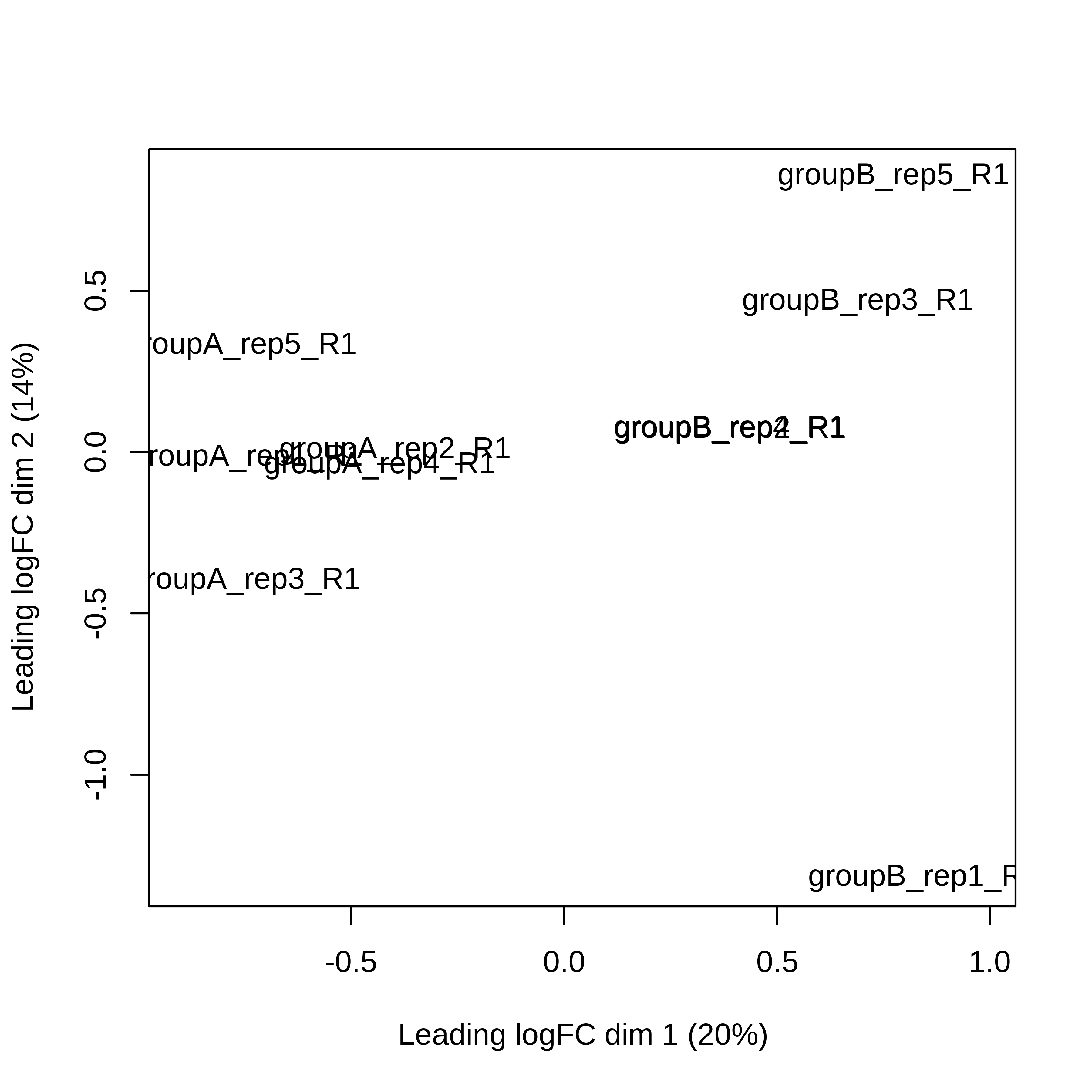
> par(mfrow = c(2,3))
> for (i in 1:ncol(dge.scaled.filtr)) plotMD(dge.scaled.filtr,column = i)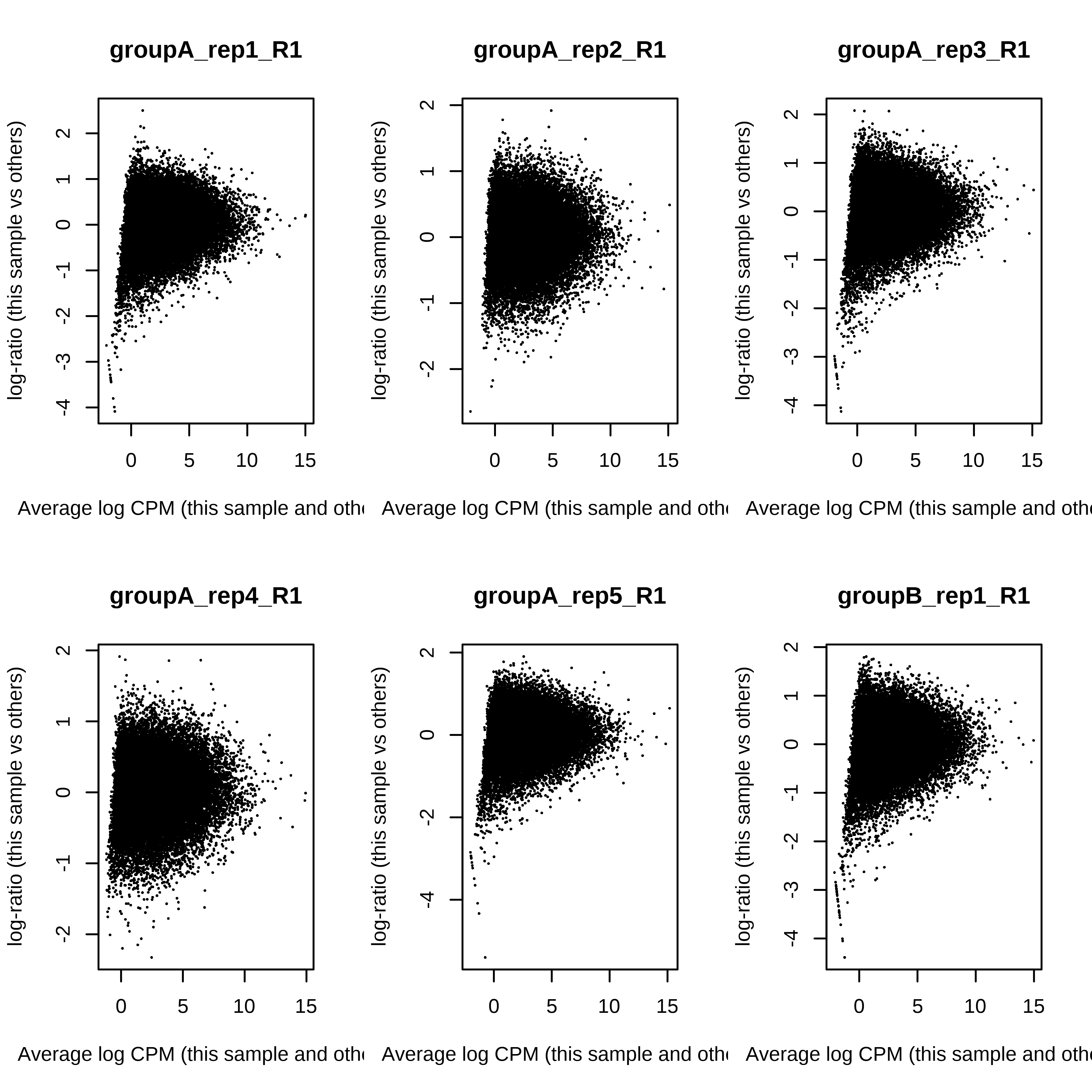
> par(mfrow = c(1,1))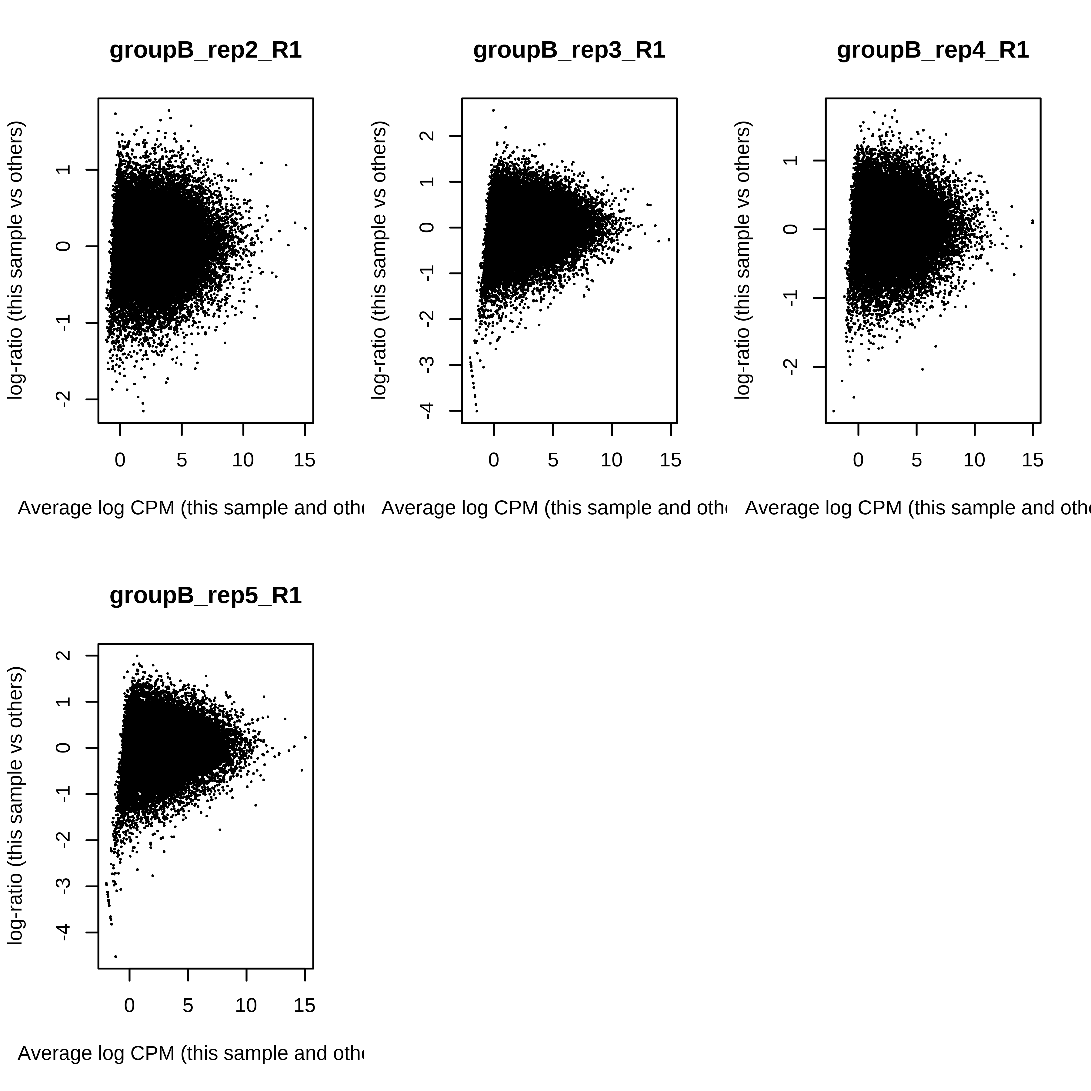
>
> design <- model.matrix(~group-1,data = dge.scaled.filtr$samples)
> colnames(design) <- gsub('group','',colnames(design))
> dge.scaled.filtr <- estimateDisp(dge.scaled.filtr,design)
>
> dge.scaled.filtr$common.dispersion
[1] 0.06575162
>
> plotBCV(dge.scaled.filtr)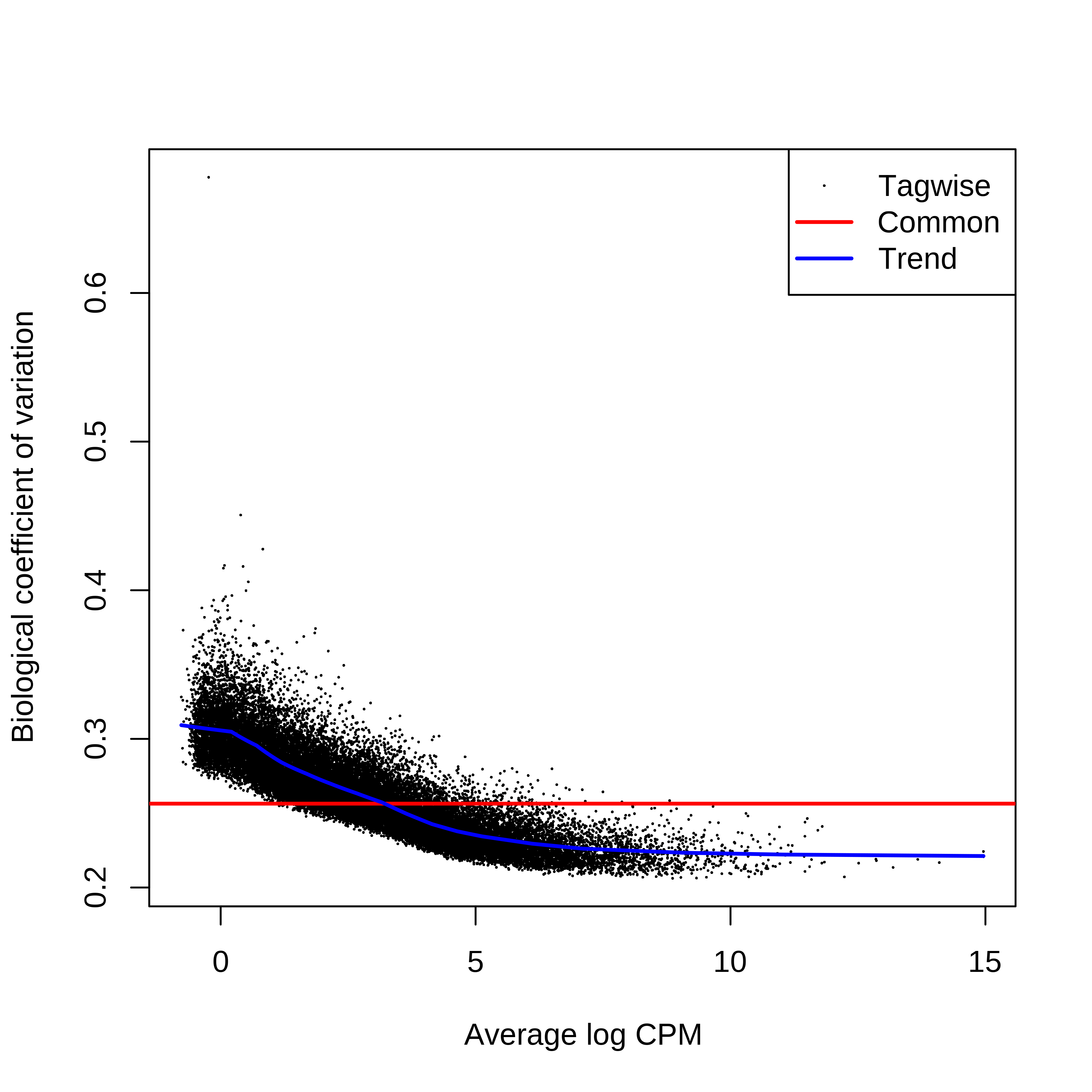
Finally, we call glmQLFit, glmQLFTest, and
plot the DTE results with an MD plot.
> fit <- glmQLFit(dge.scaled.filtr,design)
>
> plotQLDisp(fit)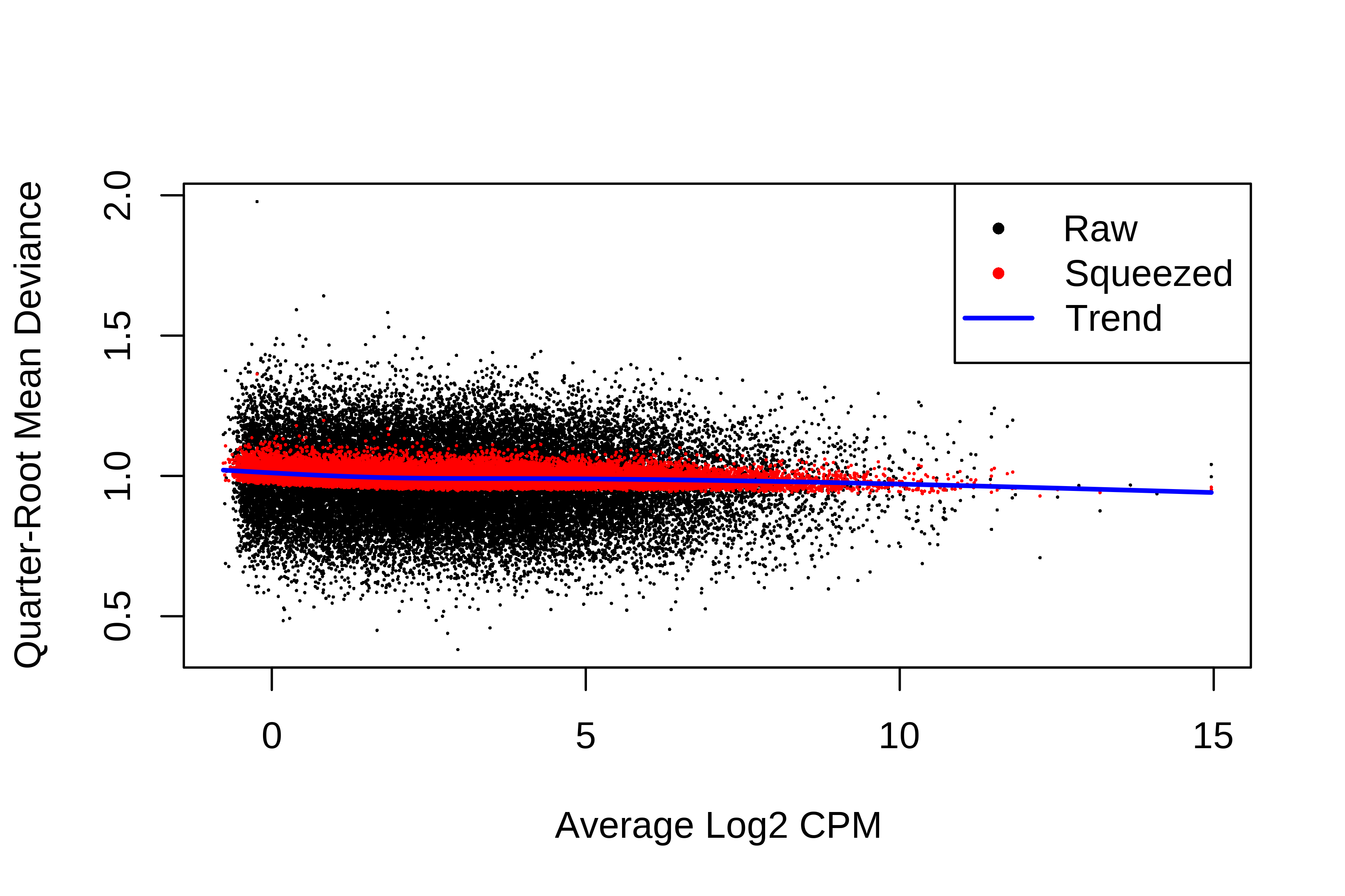
>
> summary(fit$df.prior)
   Min. 1st Qu.  Median    Mean 3rd Qu.    Max.
  39.54   39.54   39.54   39.54   39.54   39.54
>
> qlf <- glmQLFTest(fit, contrast = makeContrasts(B - A, levels = design))
>
> tt <- topTags(qlf,n = Inf)
> is.de <- decideTestsDGE(qlf)
> summary(is.de)
       -1*A 1*B
Down       1103
NotSig    26858
Up         1091
>
> plotMD(qlf, status = is.de, values = c(1, -1),
+        col = c("red","blue"), legend = "topright")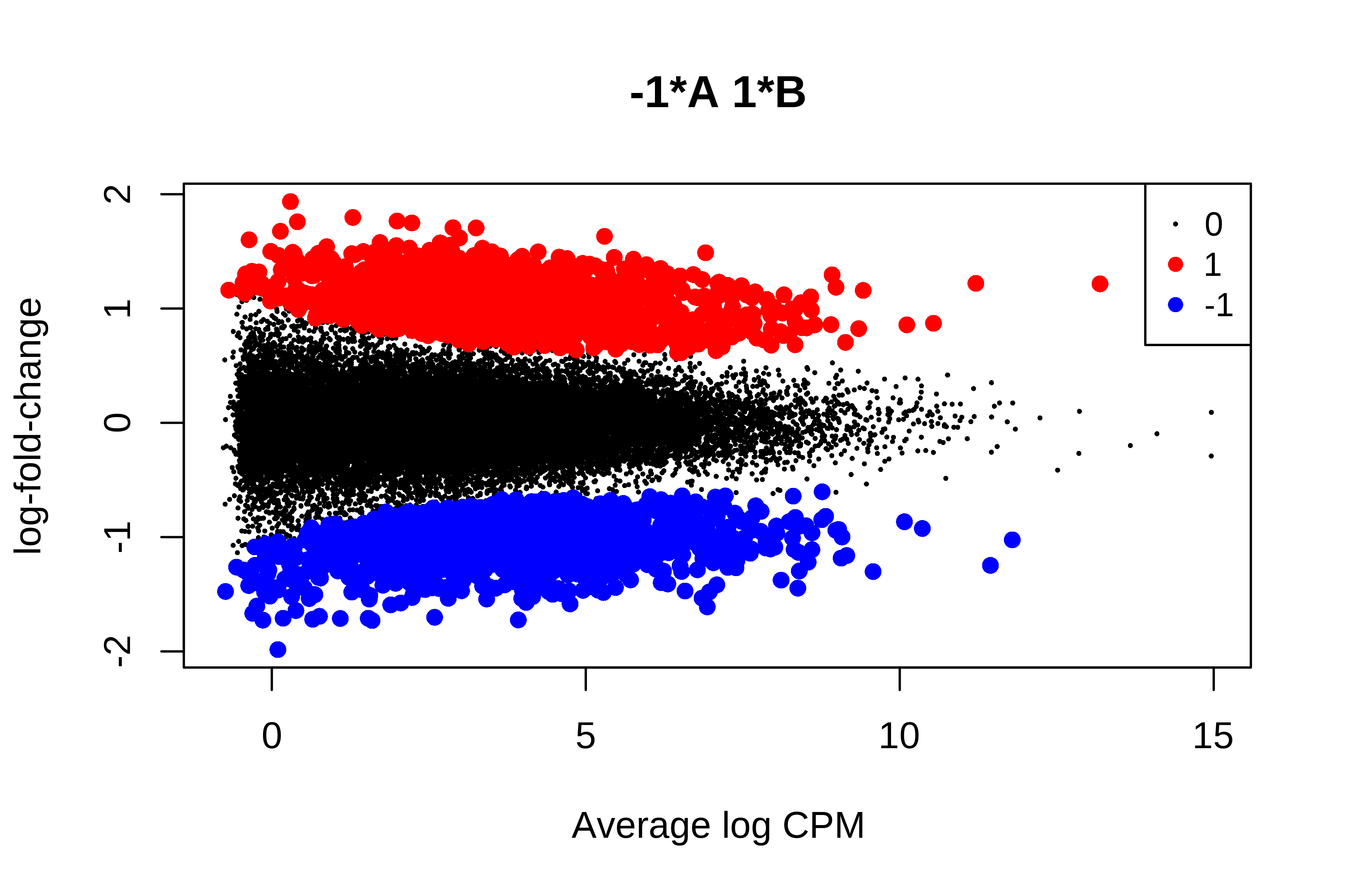
Below I tabulate the true DE status of each transcript against edgeR’s results.
> # Bringing edgeR output to dge object
> dge.scaled.filtr$genes$FDR <-
+   tt$table$FDR[match(rownames(dge.scaled.filtr$genes),rownames(tt))]
> dge.scaled.filtr$genes$logFC <-
+   tt$table$logFC[match(rownames(dge.scaled.filtr$genes),rownames(tt$table))]
> dge.scaled.filtr$genes$edgeR <-
+   is.de@.Data[,1][match(rownames(dge.scaled.filtr$genes),rownames(is.de@.Data))]
>
> table('edgeR' = dge.scaled.filtr$genes$edgeR,
+       'simulation' = dge.scaled.filtr$genes$simulation)
     simulation
edgeR    -1     0     1
   -1  1074    29     0
   0    294 26309   245
   1      0    47  1044
Then, I generate MD plots with the TP, FP, and FN status of transcripts.
> # Plotting false negatives
> dge.scaled.filtr$genes$abs.simulation <- abs(dge.scaled.filtr$genes$simulation)
> dge.scaled.filtr$genes$abs.edgeR <- abs(dge.scaled.filtr$genes$edgeR)
>
> dge.scaled.filtr$genes$TN <-
+   factor(1*with(dge.scaled.filtr$genes,abs.simulation == 0 & abs.edgeR == 0),
+          levels = c(1,0))
> dge.scaled.filtr$genes$TP <-
+   factor(1*with(dge.scaled.filtr$genes,abs.simulation == 1 & abs.edgeR == 1),
+          levels = c(1,0))
> dge.scaled.filtr$genes$FN <-
+   factor(1*with(dge.scaled.filtr$genes,abs.simulation == 1 & abs.edgeR == 0),
+          levels = c(1,0))
> dge.scaled.filtr$genes$FP <-
+   factor(1*with(dge.scaled.filtr$genes,abs.simulation == 0 & abs.edgeR == 1),
+          levels = c(1,0))
>
> tb.metrics.edger_scaled <- with(dge.scaled.filtr$genes,table(abs.simulation,abs.edgeR))
>
> message('TPR = ',tb.metrics.edger_scaled['1','1']/sum(tb.metrics.edger_scaled['1',]))
TPR = 0.797139631162966
> message('FPR = ',tb.metrics.edger_scaled['0','1']/sum(tb.metrics.edger_scaled['0',]))
FPR = 0.00288042448360811
> message('FDR = ',tb.metrics.edger_scaled['0','1']/sum(tb.metrics.edger_scaled[,'1']))
FDR = 0.0346399270738377
>
> col.tp <- c('black','red')[as.numeric(dge.scaled.filtr$genes$TP)]
> col.fn <- c('black','red')[as.numeric(dge.scaled.filtr$genes$FN)]
> col.fp <- c('black','red')[as.numeric(dge.scaled.filtr$genes$FP)]
>
> par(mfrow = c(3,1))
> plotMD(qlf,status = dge.scaled.filtr$genes$TP,main = 'True positives',col = col.tp)
> plotMD(qlf,status = dge.scaled.filtr$genes$FN,main = 'False negatives',col = col.fn)
> plotMD(qlf,status = dge.scaled.filtr$genes$FP,main = 'False positives',col = col.fp)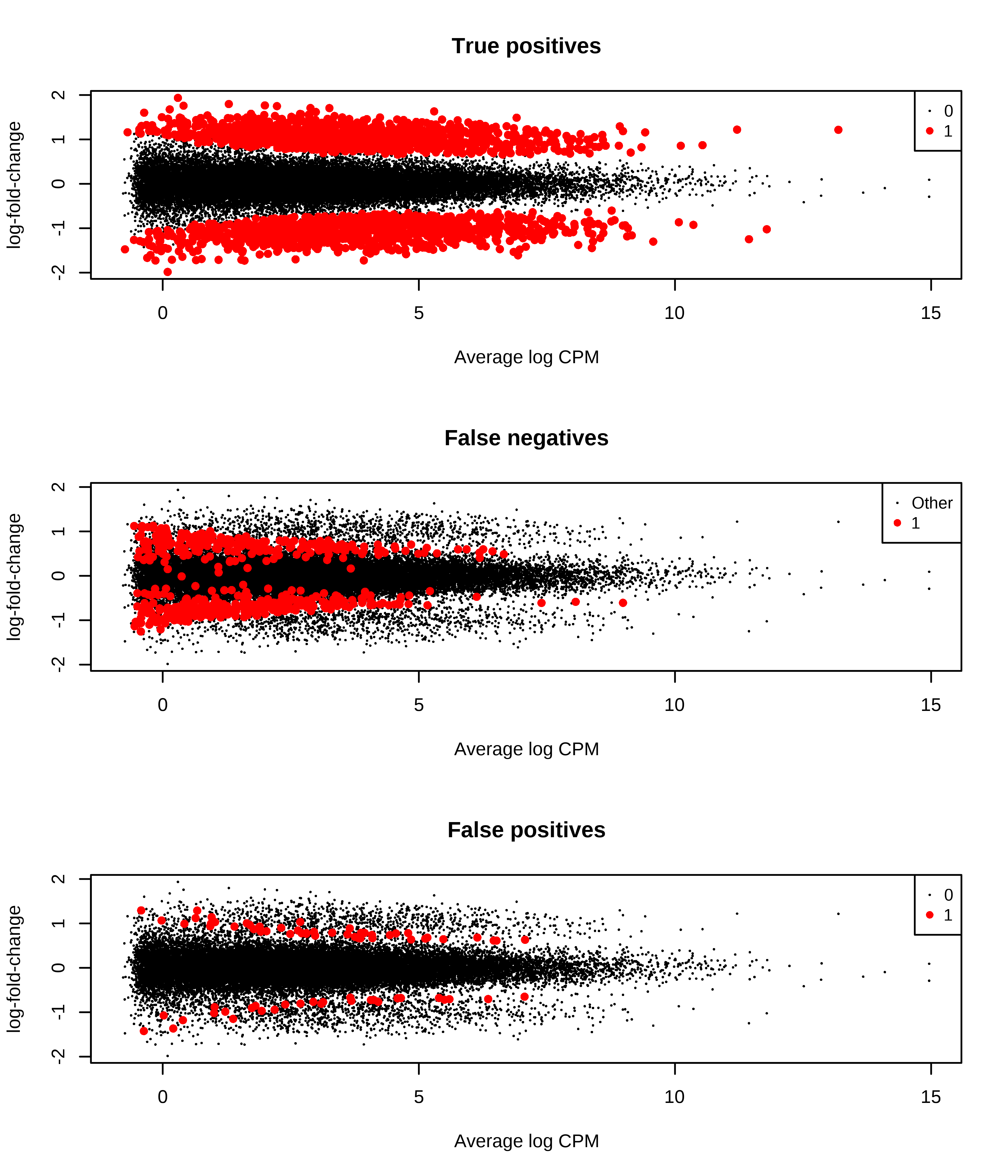
Below is a histogram of observed logFC. The histograms of truly DE should be centered around +/- 1, or +- log2(2).
> # Plotting fold changes (should be around 2)
> par(mfrow = c(1,3))
> hist(dge.scaled.filtr$genes$logFC[dge.scaled.filtr$genes$simulation == 1],
+      xlab = 'logFC',main = 'Up-regulated transcripts (log2(2))',
+      xlim = c(-2,2))
> abline(v = log2(2),col = 'red')
> hist(dge.scaled.filtr$genes$logFC[dge.scaled.filtr$genes$simulation == 0],
+      xlab = 'logFC',main = 'No DTE',xlim = c(-2,2))
> abline(v = log2(1),col = 'red')
> hist(dge.scaled.filtr$genes$logFC[dge.scaled.filtr$genes$simulation == -1],
+      xlab = 'logFC',main = 'Down-regulated transcripts (log2(1/2))',
+      xlim = c(-2,2))
> abline(v = log2(1/2),col = 'red')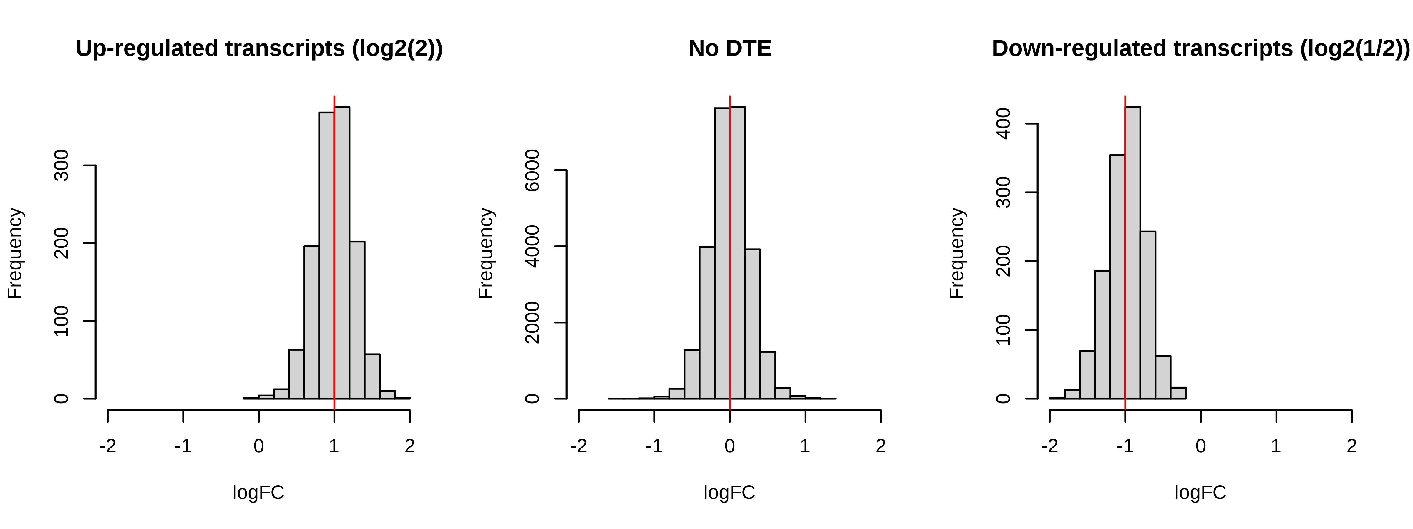
edgeR-raw
> # Creating DGEList with both raw and raw approaches
> cts.raw <- df.example.salmon$counts
>
> dge.raw <- DGEList(counts = cts.raw,
+                    samples = df.example.targets,
+                    genes = df.example.salmon$annotation)
>
> # Adding true DE status to DGEList
> dge.raw$genes$simulation <-
+   df.example.sim$status[match(rownames(dge.raw$genes),df.example.sim$TranscriptID)]
Next, I apply edgeR’s pipeline. I start by filtering lowly expressed transcripts and calculating normalization factors.
> # Applying edgeR's filterByExpr
> keep <- filterByExpr(dge.raw)
> table(keep, simulation = dge.raw$genes$simulation)
       simulation
keep       -1     0     1
  FALSE    10  5155    14
  TRUE   1525 33217  1451
>
> dge.raw.filtr <- dge.raw[keep, , keep.lib.sizes = FALSE]
> dge.raw.filtr <- calcNormFactors(dge.raw.filtr)
Below we have the MDS plot, MD plots, and BCV plot. There is a somewhat substantial variability among replicates of the same group (y-axis), despite the clear separation of groups along the x-axis. The BCV trends toward a value slightly above 0.2.
> plotMDS(dge.raw.filtr)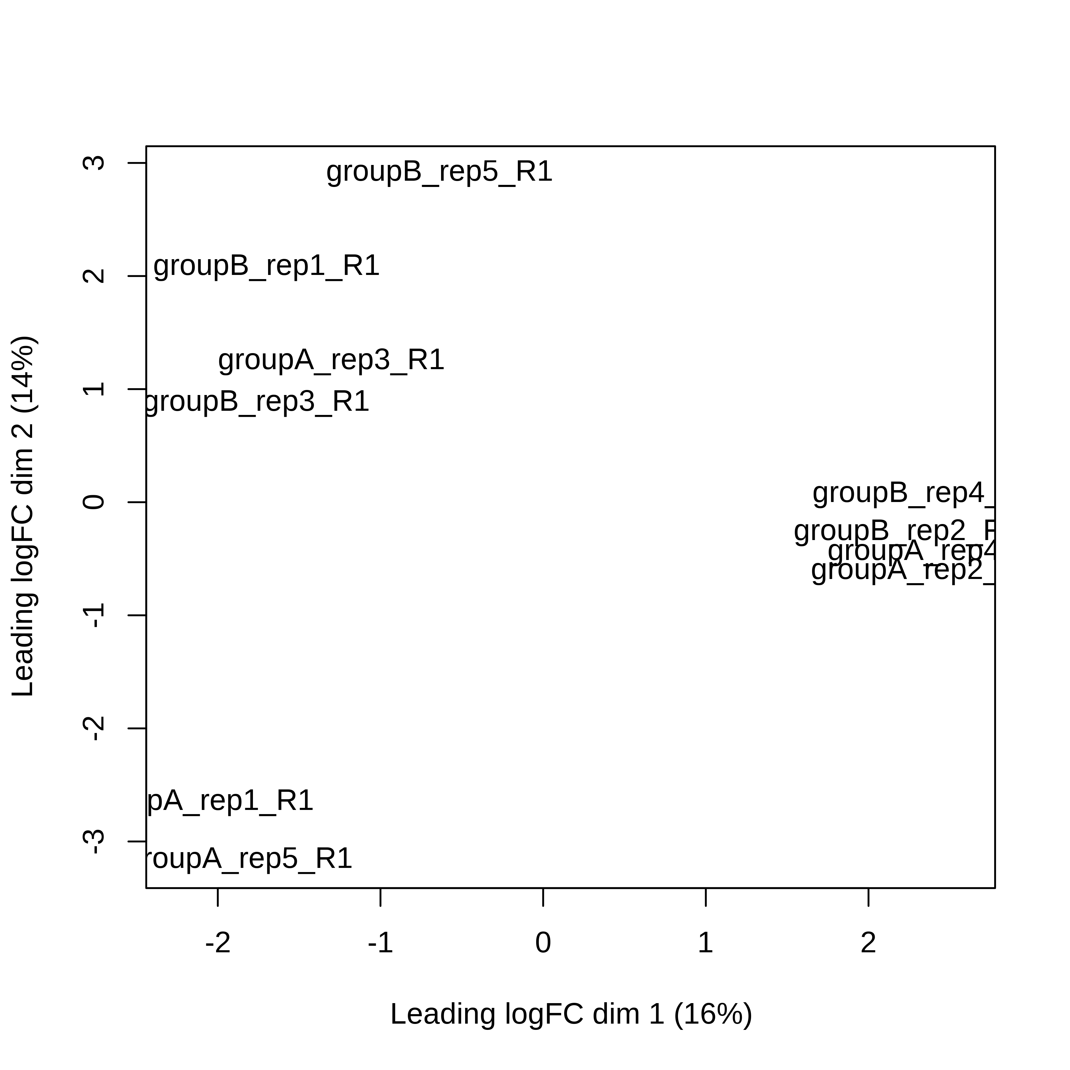
> par(mfrow = c(2,3))
> for (i in 1:ncol(dge.raw.filtr)) plotMD(dge.raw.filtr,column = i)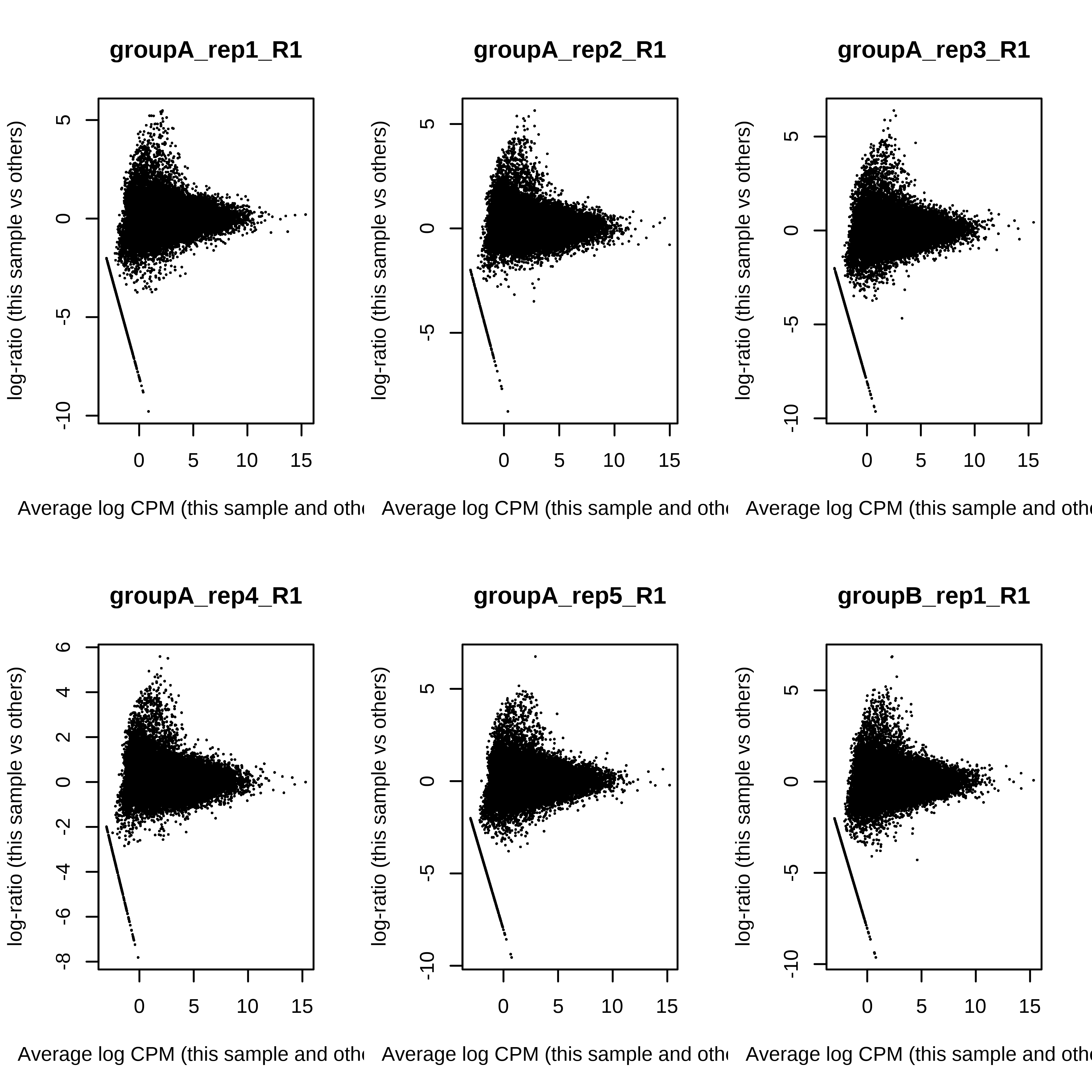
> par(mfrow = c(1,1))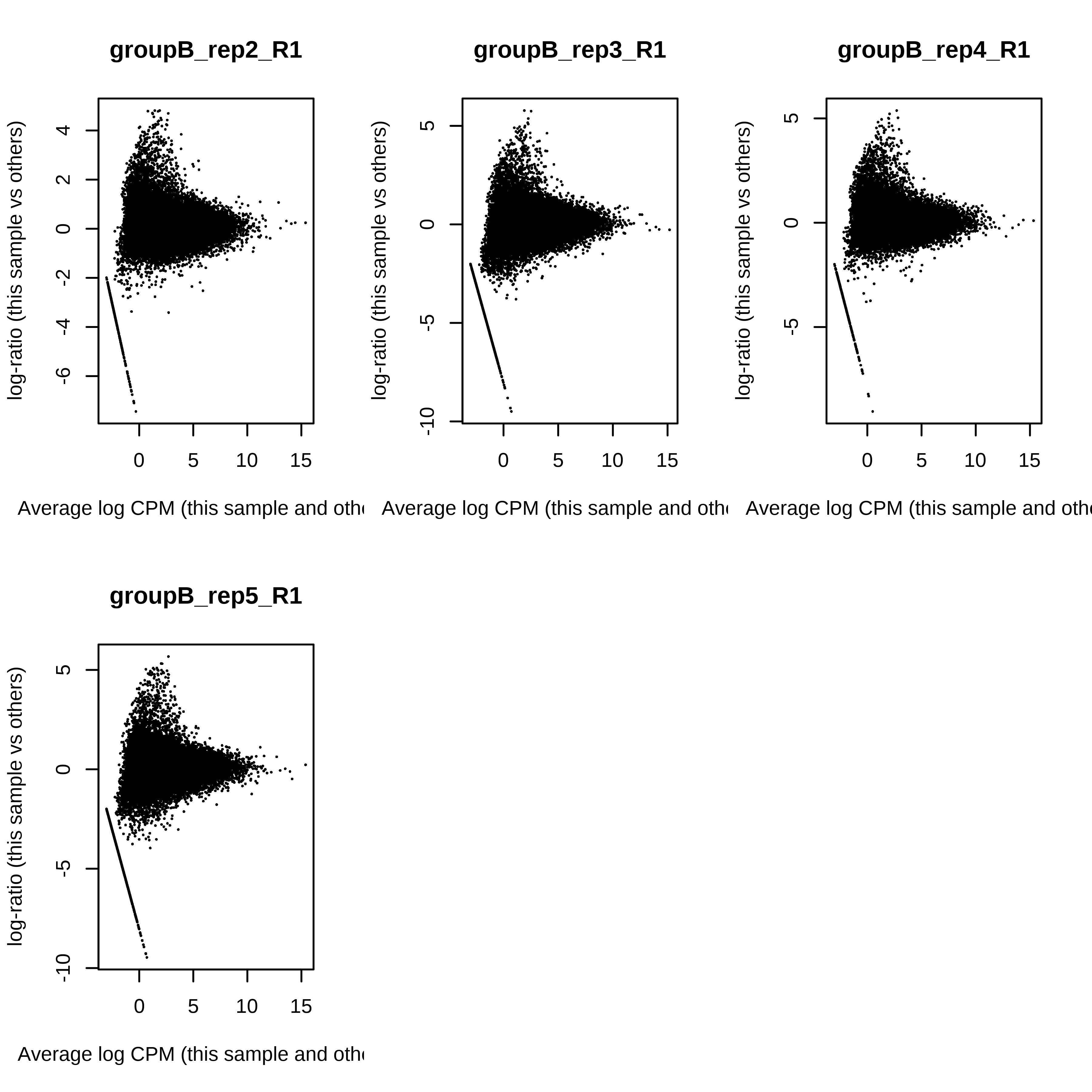
>
> design <- model.matrix(~group-1,data = dge.raw.filtr$samples)
> colnames(design) <- gsub('group','',colnames(design))
> dge.raw.filtr <- estimateDisp(dge.raw.filtr,design)
>
> dge.raw.filtr$common.dispersion
[1] 0.1877797
>
> plotBCV(dge.raw.filtr)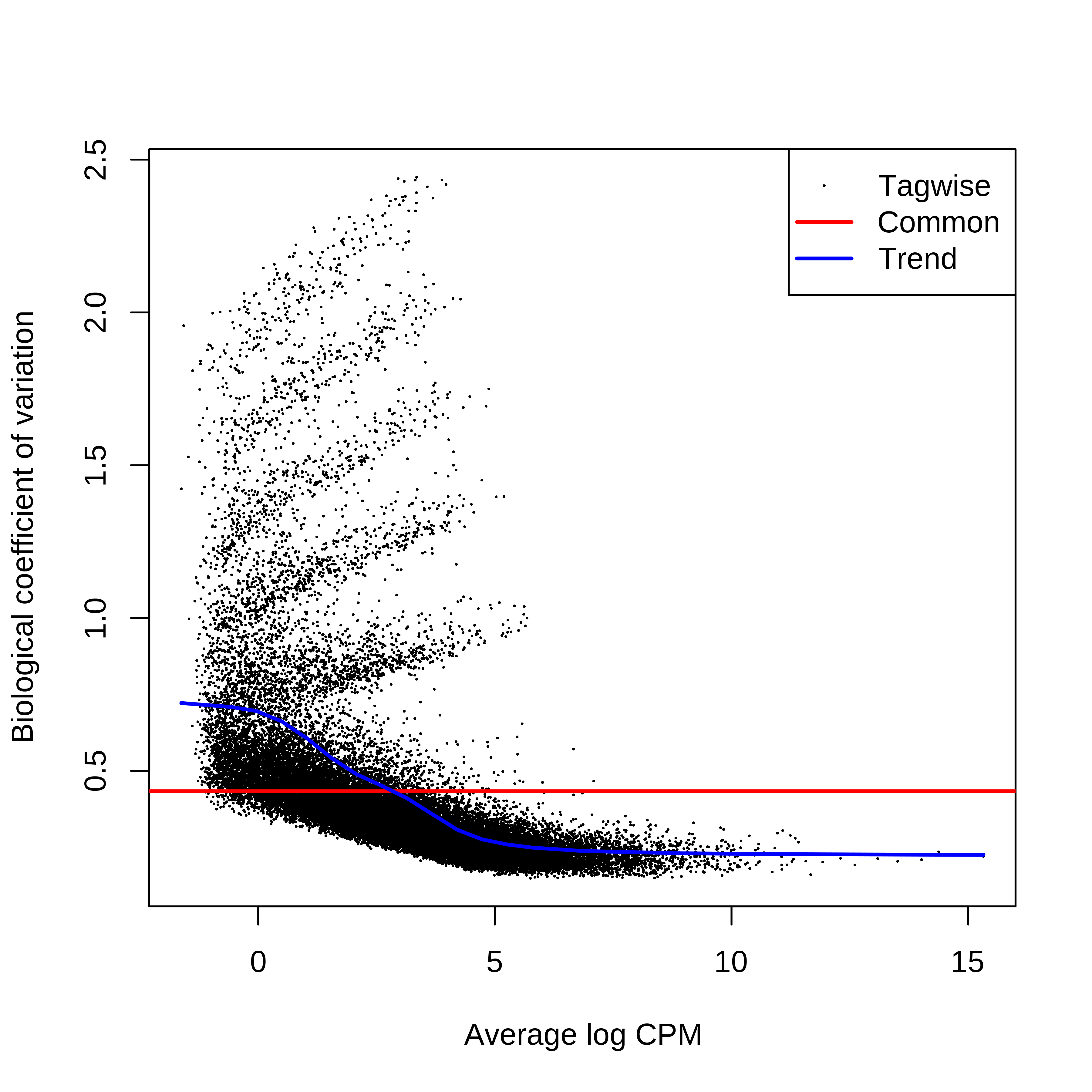
Finally, we call glmQLFit, glmQLFTest, and
plot the DTE results with an MD plot.
> fit <- glmQLFit(dge.raw.filtr,design)
>
> plotQLDisp(fit)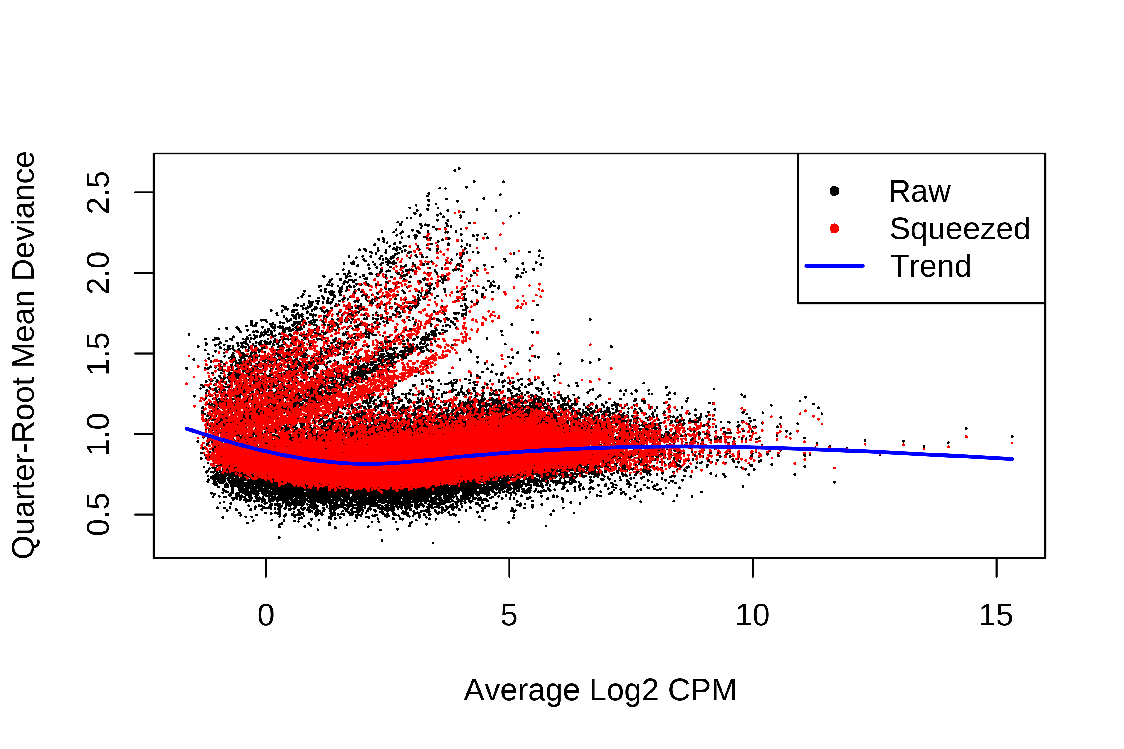
>
> summary(fit$df.prior)
   Min. 1st Qu.  Median    Mean 3rd Qu.    Max.
  4.292   4.292   4.292   4.292   4.292   4.292
>
> qlf <- glmQLFTest(fit, contrast = makeContrasts(B - A, levels = design))
>
> tt <- topTags(qlf,n = Inf)
> is.de <- decideTestsDGE(qlf)
> summary(is.de)
       -1*A 1*B
Down        742
NotSig    34715
Up          767
>
> plotMD(qlf, status = is.de, values = c(1, -1),
+        col = c("red","blue"), legend = "topright")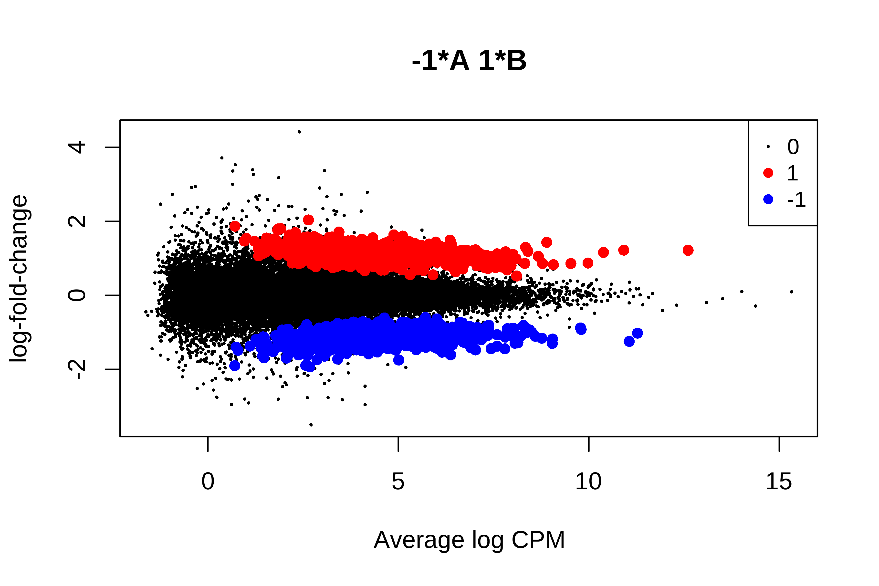
Below I tabulate the true DE status of each transcript against edgeR’s results.
> # Bringing edgeR output to dge object
> dge.raw.filtr$genes$FDR <-
+   tt$table$FDR[match(rownames(dge.raw.filtr$genes),rownames(tt))]
> dge.raw.filtr$genes$logFC <-
+   tt$table$logFC[match(rownames(dge.raw.filtr$genes),rownames(tt$table))]
> dge.raw.filtr$genes$edgeR <-
+   is.de@.Data[,1][match(rownames(dge.raw.filtr$genes),rownames(is.de@.Data))]
>
> table('edgeR' = dge.raw.filtr$genes$edgeR,
+       'simulation' = dge.raw.filtr$genes$simulation)
     simulation
edgeR    -1     0     1
   -1   737     5     0
   0    788 33197   699
   1      0    15   752
Then, I generate MD plots with the TP, FP, and FN status of transcripts.
> # Plotting false negatives
> dge.raw.filtr$genes$abs.simulation <- abs(dge.raw.filtr$genes$simulation)
> dge.raw.filtr$genes$abs.edgeR <- abs(dge.raw.filtr$genes$edgeR)
>
> dge.raw.filtr$genes$TN <-
+   factor(1*with(dge.raw.filtr$genes,abs.simulation == 0 & abs.edgeR == 0),
+          levels = c(1,0))
> dge.raw.filtr$genes$TP <-
+   factor(1*with(dge.raw.filtr$genes,abs.simulation == 1 & abs.edgeR == 1),
+          levels = c(1,0))
> dge.raw.filtr$genes$FN <-
+   factor(1*with(dge.raw.filtr$genes,abs.simulation == 1 & abs.edgeR == 0),
+          levels = c(1,0))
> dge.raw.filtr$genes$FP <-
+   factor(1*with(dge.raw.filtr$genes,abs.simulation == 0 & abs.edgeR == 1),
+          levels = c(1,0))
>
> tb.metrics.edger_raw <- with(dge.raw.filtr$genes,table(abs.simulation,abs.edgeR))
>
> message('TPR = ',tb.metrics.edger_raw['1','1']/sum(tb.metrics.edger_raw['1',]))
TPR = 0.500336021505376
> message('FPR = ',tb.metrics.edger_raw['0','1']/sum(tb.metrics.edger_raw['0',]))
FPR = 0.000602101333654454
> message('FDR = ',tb.metrics.edger_raw['0','1']/sum(tb.metrics.edger_raw[,'1']))
FDR = 0.0132538104705103
>
> col.tp <- c('black','red')[as.numeric(dge.raw.filtr$genes$TP)]
> col.fn <- c('black','red')[as.numeric(dge.raw.filtr$genes$FN)]
> col.fp <- c('black','red')[as.numeric(dge.raw.filtr$genes$FP)]
>
> par(mfrow = c(3,1))
> plotMD(qlf,status = dge.raw.filtr$genes$TP,main = 'True positives',col = col.tp)
> plotMD(qlf,status = dge.raw.filtr$genes$FN,main = 'False negatives',col = col.fn)
> plotMD(qlf,status = dge.raw.filtr$genes$FP,main = 'False positives',col = col.fp)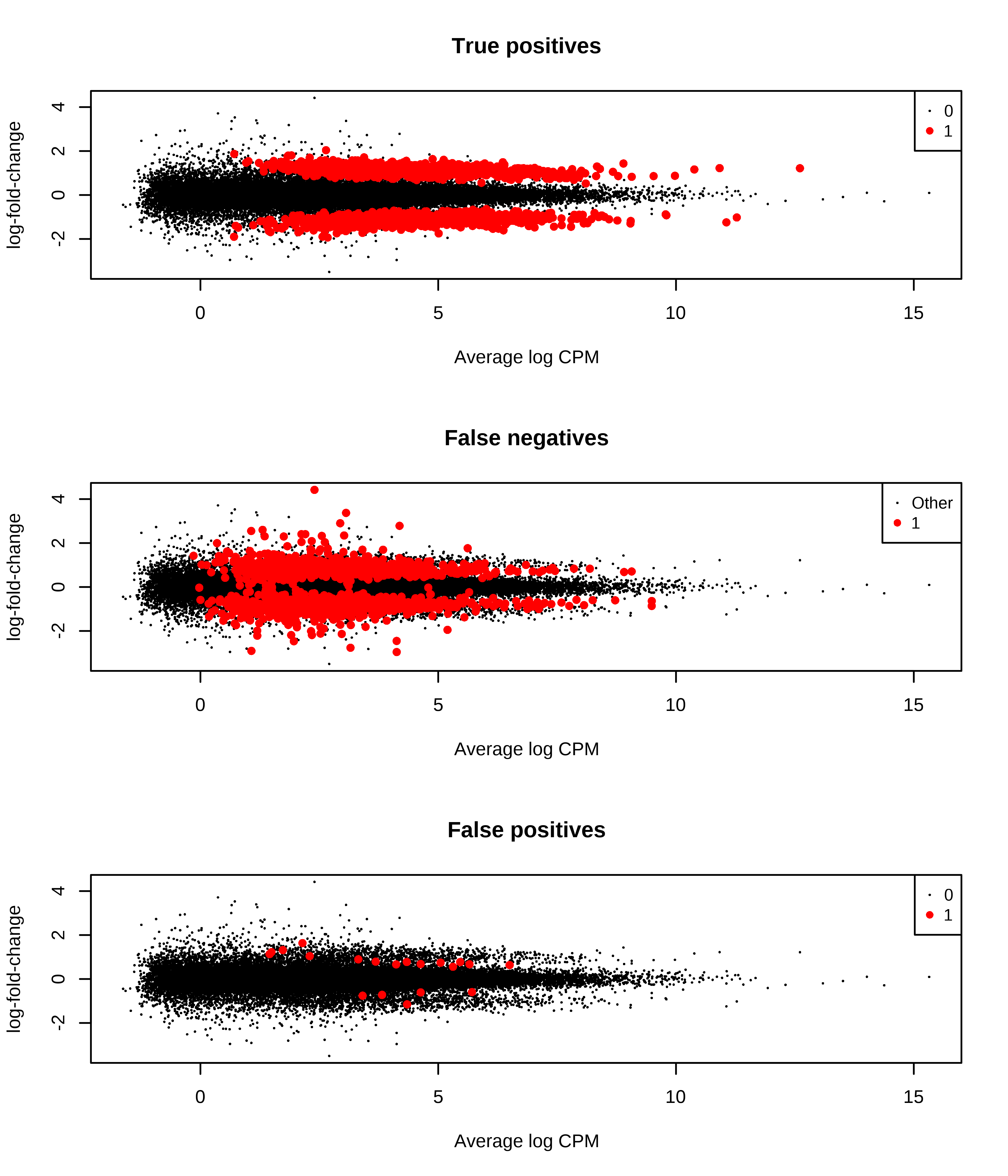
Below is a histogram of observed logFC. The histograms of truly DE should be centered around +/- 1, or +- log2(2).
> # Plotting fold changes (should be around 2)
> par(mfrow = c(1,3))
> hist(dge.raw.filtr$genes$logFC[dge.raw.filtr$genes$simulation == 1],
+      xlab = 'logFC',main = 'Up-regulated transcripts (log2(2))',
+      xlim = c(-3,3))
> abline(v = log2(2),col = 'red')
> hist(dge.raw.filtr$genes$logFC[dge.raw.filtr$genes$simulation == 0],
+      xlab = 'logFC',main = 'No DTE',xlim = c(-3,3))
> abline(v = log2(1),col = 'red')
> hist(dge.raw.filtr$genes$logFC[dge.raw.filtr$genes$simulation == -1],
+      xlab = 'logFC',main = 'Down-regulated transcripts (log2(1/2))',
+      xlim = c(-3,3))
> abline(v = log2(1/2),col = 'red')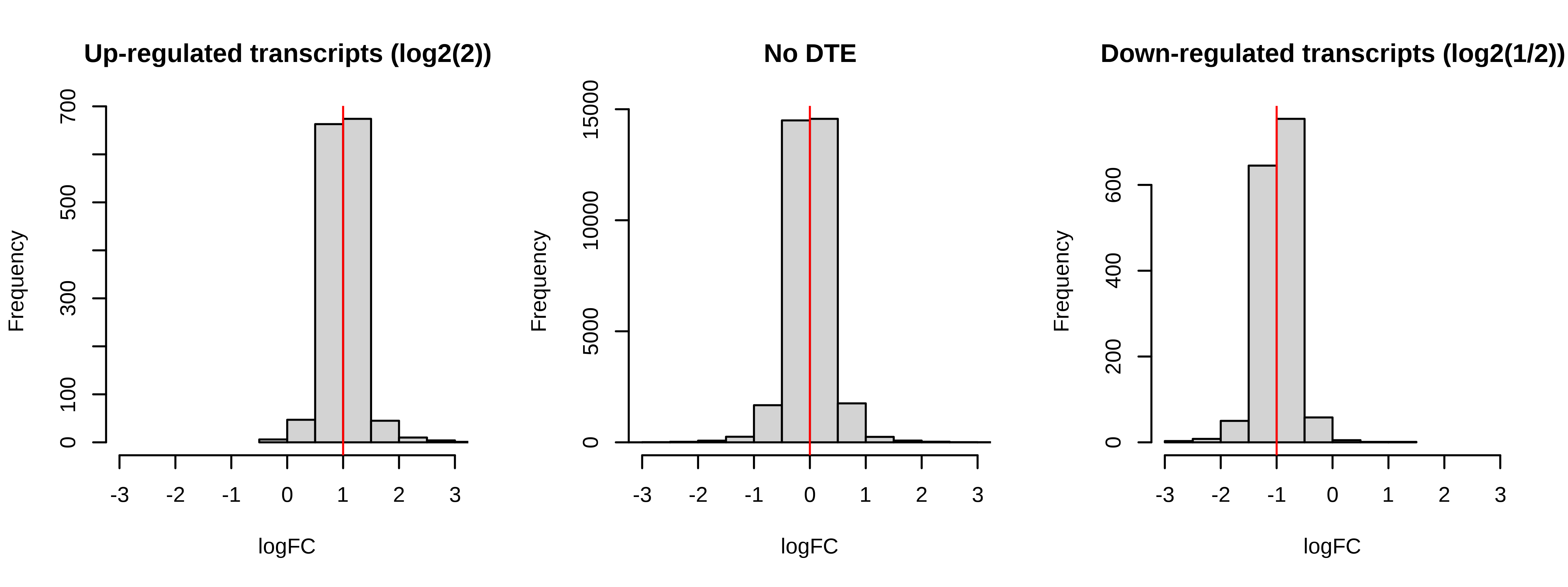
sleuth-LRT
Now I run sleuth LRT:
> # See ../rfun/ function runSleuth
> dge.sleuth_lrt <- runSleuth(targets = df.example.targets,test = 'lrt',quantifier = 'salmon')
reading in kallisto results
dropping unused factor levels
..........
normalizing est_counts
38535 targets passed the filter
normalizing tpm
merging in metadata
summarizing bootstraps
..........
fitting measurement error models
shrinkage estimation
4 NA values were found during variance shrinkage estimation due to mean observation values outside of the range used for the LOESS fit.
The LOESS fit will be repeated using exact computation of the fitted surface to extrapolate the missing values.
These are the target ids with NA values: ENSMUST00000106621.4, ENSMUST00000185239.2, ENSMUST00000195443.6, ENSMUST00000230505.2
computing variance of betas
fitting measurement error models
shrinkage estimation
3 NA values were found during variance shrinkage estimation due to mean observation values outside of the range used for the LOESS fit.
The LOESS fit will be repeated using exact computation of the fitted surface to extrapolate the missing values.
These are the target ids with NA values: ENSMUST00000106621.4, ENSMUST00000185239.2, ENSMUST00000195443.6
computing variance of betas
>
> # Plotting false negatives
> dge.sleuth_lrt$abs.simulation <-
+   abs(df.example.sim$status[match(dge.sleuth_lrt$feature,df.example.sim$TranscriptID)])
> dge.sleuth_lrt$abs.sleuth <- 1*(dge.sleuth_lrt$qval < 0.05)
>
> dge.sleuth_lrt$TN <-
+   factor(1*with(dge.sleuth_lrt,abs.simulation == 0 & abs.sleuth == 0),
+          levels = c(1,0))
> dge.sleuth_lrt$TP <-
+   factor(1*with(dge.sleuth_lrt,abs.simulation == 1 & abs.sleuth == 1),
+          levels = c(1,0))
> dge.sleuth_lrt$FN <-
+   factor(1*with(dge.sleuth_lrt,abs.simulation == 1 & abs.sleuth == 0),
+          levels = c(1,0))
> dge.sleuth_lrt$FP <-
+   factor(1*with(dge.sleuth_lrt,abs.simulation == 0 & abs.sleuth == 1),
+          levels = c(1,0))
>
> tb.metrics.sleuth_lrt <- with(dge.sleuth_lrt,table(abs.simulation,abs.sleuth))
>
> message('TPR = ',tb.metrics.sleuth_lrt['1','1']/sum(tb.metrics.sleuth_lrt['1',]))
TPR = 0.503862949277796
> message('FPR = ',tb.metrics.sleuth_lrt['0','1']/sum(tb.metrics.sleuth_lrt['0',]))
FPR = 0.000535377159119727
> message('FDR = ',tb.metrics.sleuth_lrt['0','1']/sum(tb.metrics.sleuth_lrt[,'1']))
FDR = 0.0125082290980908
sleuth-Wald
Now I run sleuth Wald:
> # See ../rfun/ function runSleuth
> dge.sleuth_wald <- runSleuth(targets = df.example.targets,test = 'wald',quantifier = 'salmon')
reading in kallisto results
dropping unused factor levels
..........
normalizing est_counts
38535 targets passed the filter
normalizing tpm
merging in metadata
summarizing bootstraps
..........
fitting measurement error models
shrinkage estimation
4 NA values were found during variance shrinkage estimation due to mean observation values outside of the range used for the LOESS fit.
The LOESS fit will be repeated using exact computation of the fitted surface to extrapolate the missing values.
These are the target ids with NA values: ENSMUST00000106621.4, ENSMUST00000185239.2, ENSMUST00000195443.6, ENSMUST00000230505.2
computing variance of betas
>
> # Plotting false negatives
> dge.sleuth_wald$abs.simulation <-
+   abs(df.example.sim$status[match(dge.sleuth_wald$feature,df.example.sim$TranscriptID)])
> dge.sleuth_wald$abs.sleuth <- 1*(dge.sleuth_wald$qval < 0.05)
>
> dge.sleuth_wald$TN <-
+   factor(1*with(dge.sleuth_wald,abs.simulation == 0 & abs.sleuth == 0),
+          levels = c(1,0))
> dge.sleuth_wald$TP <-
+   factor(1*with(dge.sleuth_wald,abs.simulation == 1 & abs.sleuth == 1),
+          levels = c(1,0))
> dge.sleuth_wald$FN <-
+   factor(1*with(dge.sleuth_wald,abs.simulation == 1 & abs.sleuth == 0),
+          levels = c(1,0))
> dge.sleuth_wald$FP <-
+   factor(1*with(dge.sleuth_wald,abs.simulation == 0 & abs.sleuth == 1),
+          levels = c(1,0))
>
> tb.metrics.sleuth_wald <- with(dge.sleuth_wald,table(abs.simulation,abs.sleuth))
>
> message('TPR = ',tb.metrics.sleuth_wald['1','1']/sum(tb.metrics.sleuth_wald['1',]))
TPR = 0.616056432650319
> message('FPR = ',tb.metrics.sleuth_wald['0','1']/sum(tb.metrics.sleuth_wald['0',]))
FPR = 0.00169066471300966
> message('FDR = ',tb.metrics.sleuth_wald['0','1']/sum(tb.metrics.sleuth_wald[,'1']))
FDR = 0.0316789862724393
Swish
Now I run Swish:
> # See ../rfun/ function runSwish
> df.example.targets.swish <- df.example.targets
> df.example.targets.swish$group %<>% as.factor()
>
> dge.swish <- runSwish(targets = df.example.targets.swish,quantifier = 'salmon')
importing quantifications
reading in files with read_tsv
1 2 3 4 5 6 7 8 9 10
found matching transcriptome:
[ GENCODE - Mus musculus - release M27 ]
loading existing TxDb created: 2022-04-05 23:03:51
Loading required package: GenomicFeatures
Loading required package: BiocGenerics

Attaching package: 'BiocGenerics'

The following object is masked from 'package:limma':

    plotMA

The following objects are masked from 'package:stats':

    IQR, mad, sd, var, xtabs

The following objects are masked from 'package:base':

    anyDuplicated, aperm, append, as.data.frame, basename, cbind,
    colnames, dirname, do.call, duplicated, eval, evalq, Filter, Find,
    get, grep, grepl, intersect, is.unsorted, lapply, Map, mapply,
    match, mget, order, paste, pmax, pmax.int, pmin, pmin.int,
    Position, rank, rbind, Reduce, rownames, sapply, setdiff, sort,
    table, tapply, union, unique, unsplit, which.max, which.min

Loading required package: S4Vectors
Loading required package: stats4

Attaching package: 'S4Vectors'

The following object is masked from 'package:plyr':

    rename

The following objects are masked from 'package:data.table':

    first, second

The following objects are masked from 'package:base':

    expand.grid, I, unname

Loading required package: IRanges

Attaching package: 'IRanges'

The following object is masked from 'package:purrr':

    reduce

The following object is masked from 'package:plyr':

    desc

The following object is masked from 'package:data.table':

    shift

Loading required package: GenomeInfoDb
Loading required package: GenomicRanges

Attaching package: 'GenomicRanges'

The following object is masked from 'package:magrittr':

    subtract

Loading required package: AnnotationDbi
Loading required package: Biobase
Welcome to Bioconductor

    Vignettes contain introductory material; view with
    'browseVignettes()'. To cite Bioconductor, see
    'citation("Biobase")', and for packages 'citation("pkgname")'.

loading existing transcript ranges created: 2022-04-05 23:03:52
fetching genome info for GENCODE
Warning in valid.GenomicRanges.seqinfo(x, suggest.trim = TRUE): GRanges object contains 87 out-of-bound ranges located on sequences
  chr4, chr8, chr13, chr14, and chr17. Note that ranges located on a
  sequence whose length is unknown (NA) or on a circular sequence are not
  considered out-of-bound (use seqlengths() and isCircular() to get the
  lengths and circularity flags of the underlying sequences). You can use
  trim() to trim these ranges. See ?`trim,GenomicRanges-method` for more
  information.
>
> # Plotting false negatives
> dge.swish$abs.simulation <-
+   abs(df.example.sim$status[match(dge.swish$feature,df.example.sim$TranscriptID)])
> dge.swish$abs.swish <- 1*(dge.swish$qvalue < 0.05)
>
> dge.swish$TN <-
+   factor(1*with(dge.swish,abs.simulation == 0 & abs.swish == 0),
+          levels = c(1,0))
> dge.swish$TP <-
+   factor(1*with(dge.swish,abs.simulation == 1 & abs.swish == 1),
+          levels = c(1,0))
> dge.swish$FN <-
+   factor(1*with(dge.swish,abs.simulation == 1 & abs.swish == 0),
+          levels = c(1,0))
> dge.swish$FP <-
+   factor(1*with(dge.swish,abs.simulation == 0 & abs.swish == 1),
+          levels = c(1,0))
>
> tb.metrics.swish <- with(dge.swish,table(abs.simulation,abs.swish))
>
> message('TPR = ',tb.metrics.swish['1','1']/sum(tb.metrics.swish['1',]))
TPR = 0.467423989308386
> message('FPR = ',tb.metrics.swish['0','1']/sum(tb.metrics.swish['0',]))
FPR = 0.00168694690265487
> message('FDR = ',tb.metrics.swish['0','1']/sum(tb.metrics.swish[,'1']))
FDR = 0.0417808219178082
Simulation Results
Here I present the results from the simulation study. I have written
a function to summarize the results of each simulation scenario (see
function summarizeSimulation in
../code/pkg/R/simulation-summary.R). Please refer to the
caption of each figure for a description of each analysis.
Data setup and loading results
Below I set up the file paths.
> path.fdr <-
+   list.files('../output/simulation/summary','fdr.tsv.gz',recursive = TRUE,full.names = TRUE)
> path.metrics <-
+   list.files('../output/simulation/summary','metrics.tsv.gz',recursive = TRUE,full.names = TRUE)
> path.time <-
+   list.files('../output/simulation/summary','time.tsv.gz',recursive = TRUE,full.names = TRUE)
> path.quantile <-
+   list.files('../output/simulation/summary','quantile.tsv.gz',recursive = TRUE,full.names = TRUE)
> path.pvalue <-
+   list.files('../output/simulation/summary','pvalue.tsv.gz',recursive = TRUE,full.names = TRUE)
> path.overdispersion <-
+   list.files('../output/simulation/summary','overdispersion.tsv.gz',recursive = TRUE,full.names = TRUE)
Loading all summarized results below. Because these datasets are
quite large, I use cache=TRUE to save time when rendering
this page.
> # Loading datasets
> dt.fdr <- do.call(rbind,lapply(path.fdr,fread))
> dt.metrics <- do.call(rbind,lapply(path.metrics,fread))
> dt.time <- do.call(rbind,lapply(path.time,fread))
> dt.quantile <- do.call(rbind,lapply(path.quantile,fread))
> dt.pvalue <- do.call(rbind,lapply(path.pvalue,fread))
> dt.overdispersion <- do.call(rbind,lapply(path.overdispersion,fread))
Warning: The above code chunk cached its results, but
it won’t be re-run if previous chunks it depends on are updated. If you
need to use caching, it is highly recommended to also set
knitr::opts_chunk$set(autodep = TRUE) at the top of the
file (in a chunk that is not cached). Alternatively, you can customize
the option dependson for each individual chunk that is
cached. Using either autodep or dependson will
remove this warning. See the
knitr cache options for more details.
Some data wrangling below.
> # Changing labels
> dt.fdr$TxPerGene %<>%
+   mapvalues(from = paste0(c(2, 3, 4, 5, 9999), 'TxPerGene'),
+             to = c(paste0("#Tx/Gene = ", c(2, 3, 4, 5)), 'All Transcripts'))
> dt.fdr$LibsPerGroup %<>%
+   mapvalues(from = paste0(c(3, 5), 'libsPerGroup'),
+             to = paste0('#Lib/Group = ', c(3, 5)))
> dt.fdr$Quantifier %<>% mapvalues(from = 'salmon', to = 'Salmon')
> dt.fdr$Length %<>% mapvalues(from = paste0('readlen-', seq(50, 150, 25)),
+                              to = paste0(seq(50, 150, 25), 'bp'))
>
> dt.metrics$TxPerGene %<>%
+   mapvalues(from = paste0(c(2, 3, 4, 5, 9999), 'TxPerGene'),
+             to = c(paste0("#Tx/Gene = ", c(2, 3, 4, 5)), 'All Transcripts'))
> dt.metrics$LibsPerGroup %<>%
+   mapvalues(from = paste0(c(3, 5), 'libsPerGroup'),
+             to = paste0('#Lib/Group = ', c(3, 5)))
> dt.metrics$Quantifier %<>% mapvalues(from = 'salmon', to = 'Salmon')
> dt.metrics$Length %<>% mapvalues(from = paste0('readlen-', seq(50, 150, 25)),
+                                  to = paste0(seq(50, 150, 25), 'bp'))
>
> dt.time$TxPerGene %<>%
+   mapvalues(from = paste0(c(2, 3, 4, 5, 9999), 'TxPerGene'),
+             to = c(paste0("#Tx/Gene = ", c(2, 3, 4, 5)), 'All Transcripts'))
> dt.time$LibsPerGroup %<>%
+   mapvalues(from = paste0(c(3, 5), 'libsPerGroup'),
+             to = paste0('#Lib/Group = ', c(3, 5)))
> dt.time$Quantifier %<>% mapvalues(from = 'salmon', to = 'Salmon')
> dt.time$Length %<>% mapvalues(from = paste0('readlen-', seq(50, 150, 25)),
+                               to = paste0(seq(50, 150, 25), 'bp'))
>
> dt.quantile$TxPerGene %<>%
+   mapvalues(from = paste0(c(2, 3, 4, 5, 9999), 'TxPerGene'),
+             to = c(paste0("#Tx/Gene = ", c(2, 3, 4, 5)), 'All Transcripts'))
> dt.quantile$LibsPerGroup %<>%
+   mapvalues(from = paste0(c(3, 5), 'libsPerGroup'),
+             to = paste0('#Lib/Group = ', c(3, 5)))
> dt.quantile$Quantifier %<>% mapvalues(from = 'salmon', to = 'Salmon')
> dt.quantile$Length %<>% mapvalues(from = paste0('readlen-', seq(50, 150, 25)),
+                                   to = paste0(seq(50, 150, 25), 'bp'))
>
> dt.pvalue$TxPerGene %<>%
+   mapvalues(from = paste0(c(2, 3, 4, 5, 9999), 'TxPerGene'),
+             to = c(paste0("#Tx/Gene = ", c(2, 3, 4, 5)), 'All Transcripts'))
> dt.pvalue$LibsPerGroup %<>%
+   mapvalues(from = paste0(c(3, 5), 'libsPerGroup'),
+             to = paste0('#Lib/Group = ', c(3, 5)))
> dt.pvalue$Quantifier %<>% mapvalues(from = 'salmon', to = 'Salmon')
> dt.pvalue$Length %<>% mapvalues(from = paste0('readlen-', seq(50, 150, 25)),
+                                 to = paste0(seq(50, 150, 25), 'bp'))
>
> dt.overdispersion$TxPerGene %<>%
+   mapvalues(from = paste0(c(2, 3, 4, 5, 9999), 'TxPerGene'),
+             to = c(paste0("#Tx/Gene = ", c(2, 3, 4, 5)), 'All Transcripts'))
> dt.overdispersion$LibsPerGroup %<>%
+   mapvalues(from = paste0(c(3, 5), 'libsPerGroup'),
+             to = paste0('#Lib/Group = ', c(3, 5)))
> dt.overdispersion$Quantifier %<>% mapvalues(from = 'salmon', to = 'Salmon')
> dt.overdispersion$Length %<>% mapvalues(from = paste0('readlen-', seq(50, 150, 25)),
+                                         to = paste0(seq(50, 150, 25), 'bp'))
I use the functions below to produce the histogram plot shown in this report and to quickly subset data tables for specific scenarios:
> cleanPlot <- function(x,fig){
+ if (x == max(seq_along(fig))) {
+ y <- fig[[x]]
+ } else{
+ y <- fig[[x]] + theme(axis.title.x = element_blank(),
+ axis.text.x = element_blank(),
+ axis.ticks.x = element_blank())
+ }
+ if (x > 1) {
+ y <- y + theme(strip.background.x = element_blank(),
+ strip.text.x = element_blank())
+ }
+ return(y)
+ }
>
> subsetDT <- function(x,scenario,panel = NULL,tx.per.gene = NULL, plot = TRUE){
+ if(isTRUE(plot)){
+ if(panel %in% c('A','B')){
+ out <- x[Genome == scenario['genome'] &
+ FC == ifelse(panel == 'A','fc2','fc1') &
+ Length == scenario['length'] &
+ Reads == scenario['read'] &
+ Quantifier == scenario['quantifier'] &
+ Scenario == scenario['scenario'],]
+ } else{
+ out <- x[Genome == scenario['genome'] &
+ FC == 'fc1' &
+ Length == scenario['length'] &
+ Reads == scenario['read'] &
+ Quantifier == scenario['quantifier'] &
+ Scenario == scenario['scenario'] &
+ TxPerGene == tx.per.gene ,]
+ }
+ } else{
+ out <- x[Genome == scenario['genome'] &
+ FC == 'fc2' &
+ Quantifier == scenario['quantifier'] &
+ TxPerGene == scenario['txpergene'],]
+ }
+ return(out)
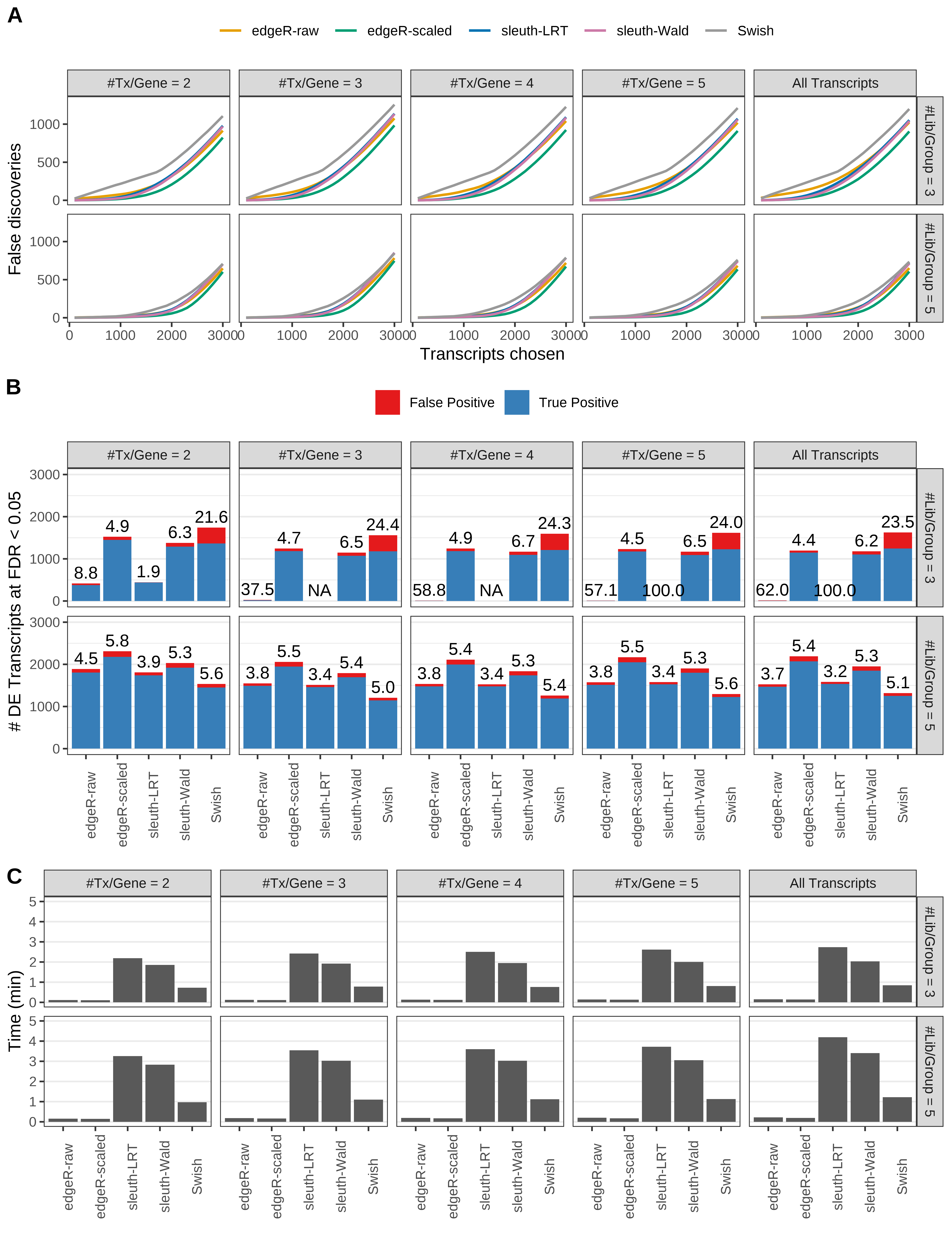
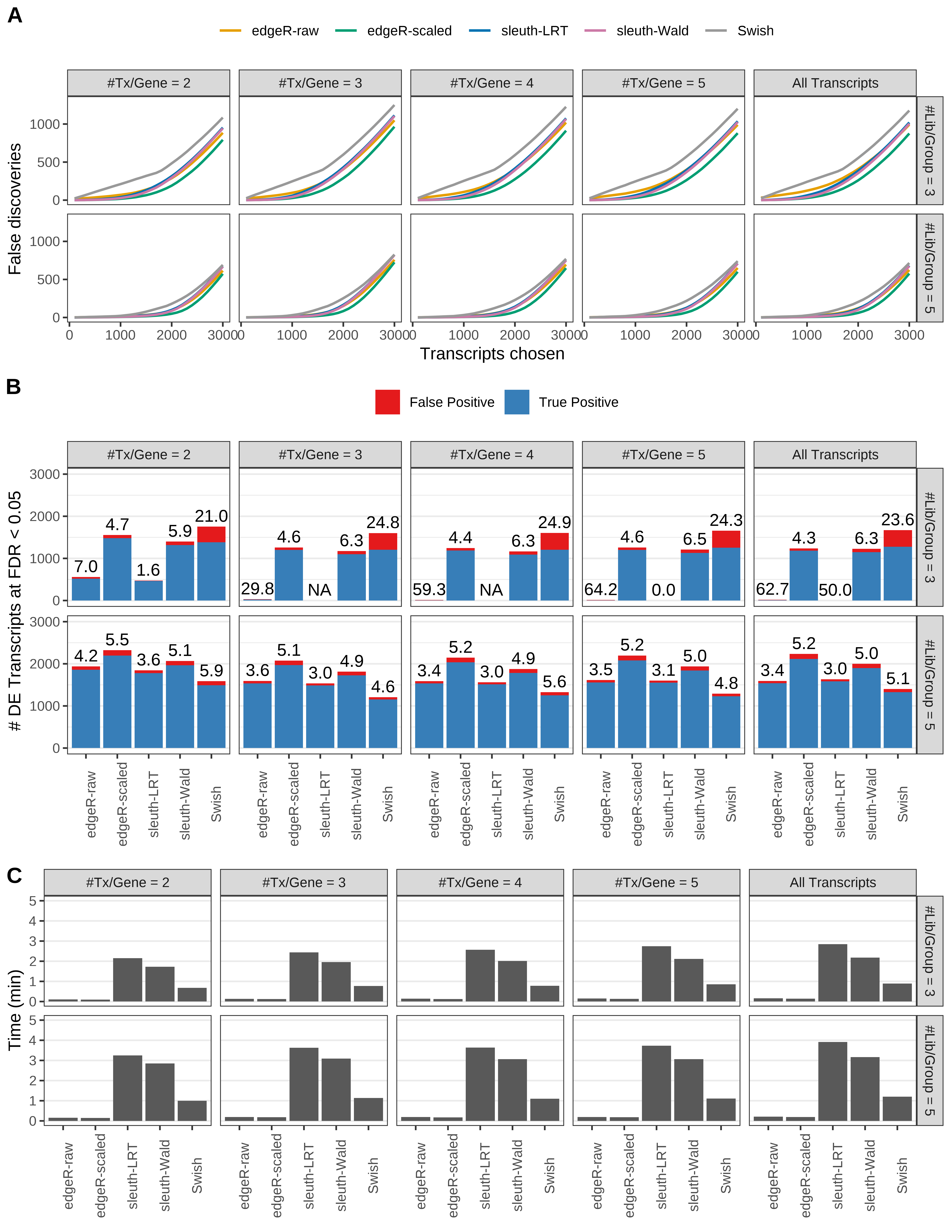
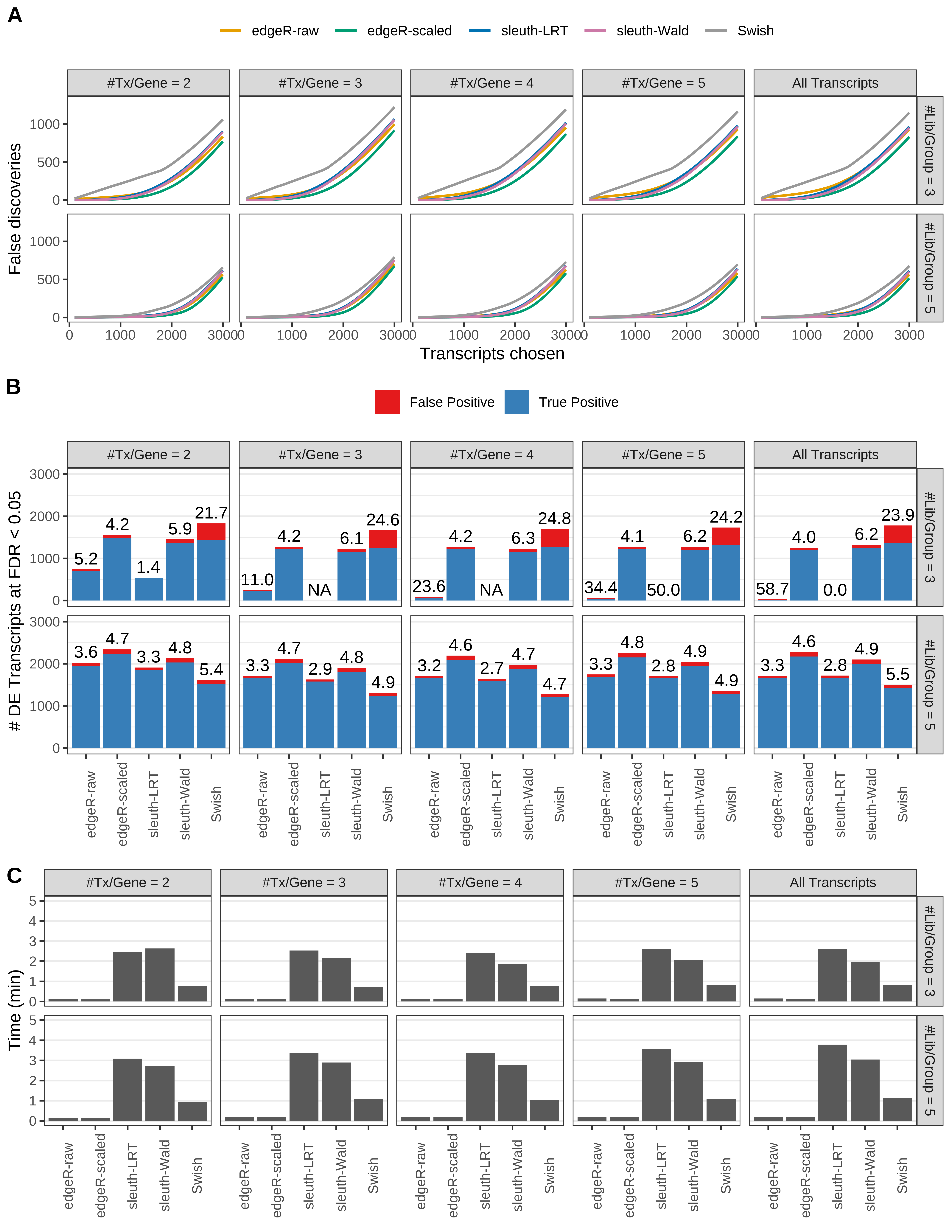
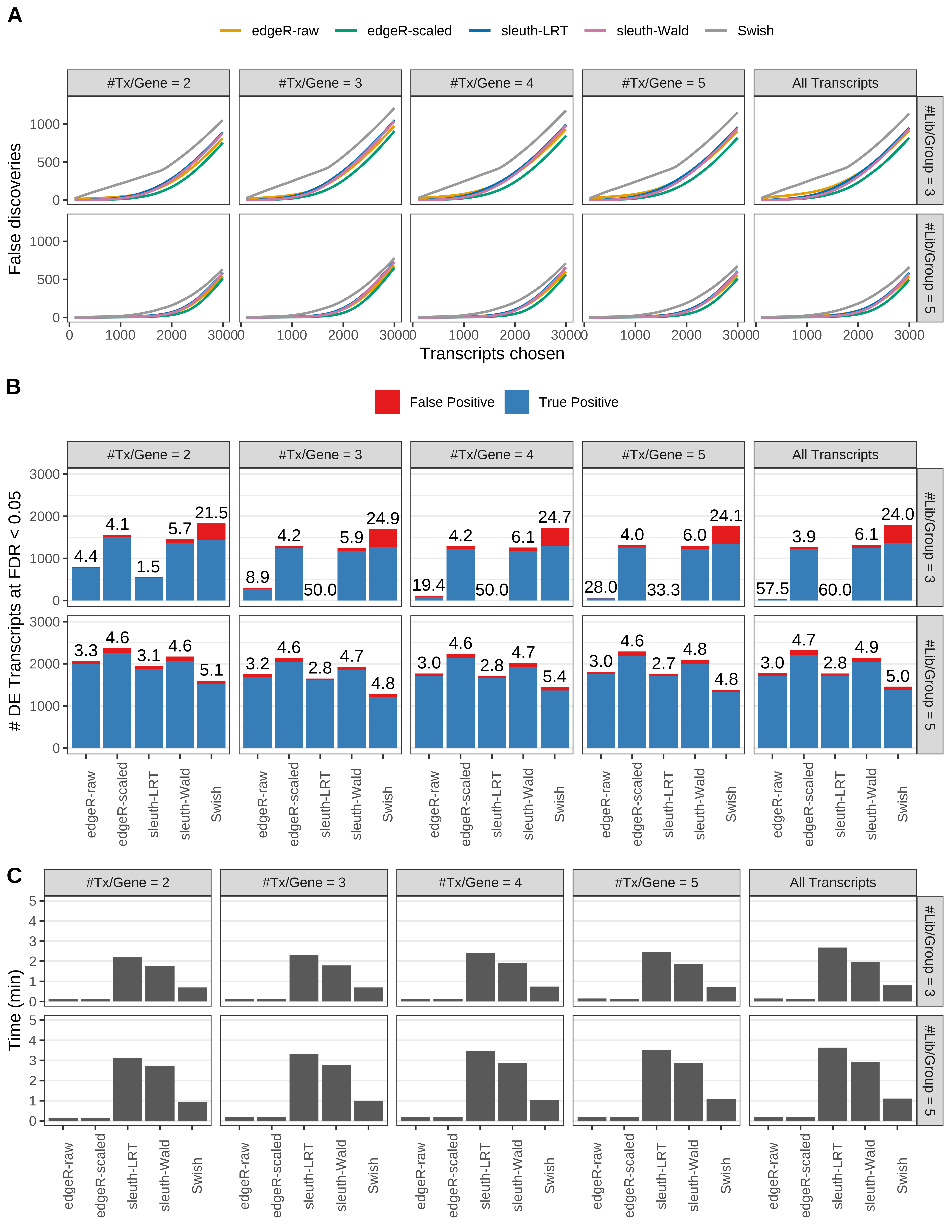
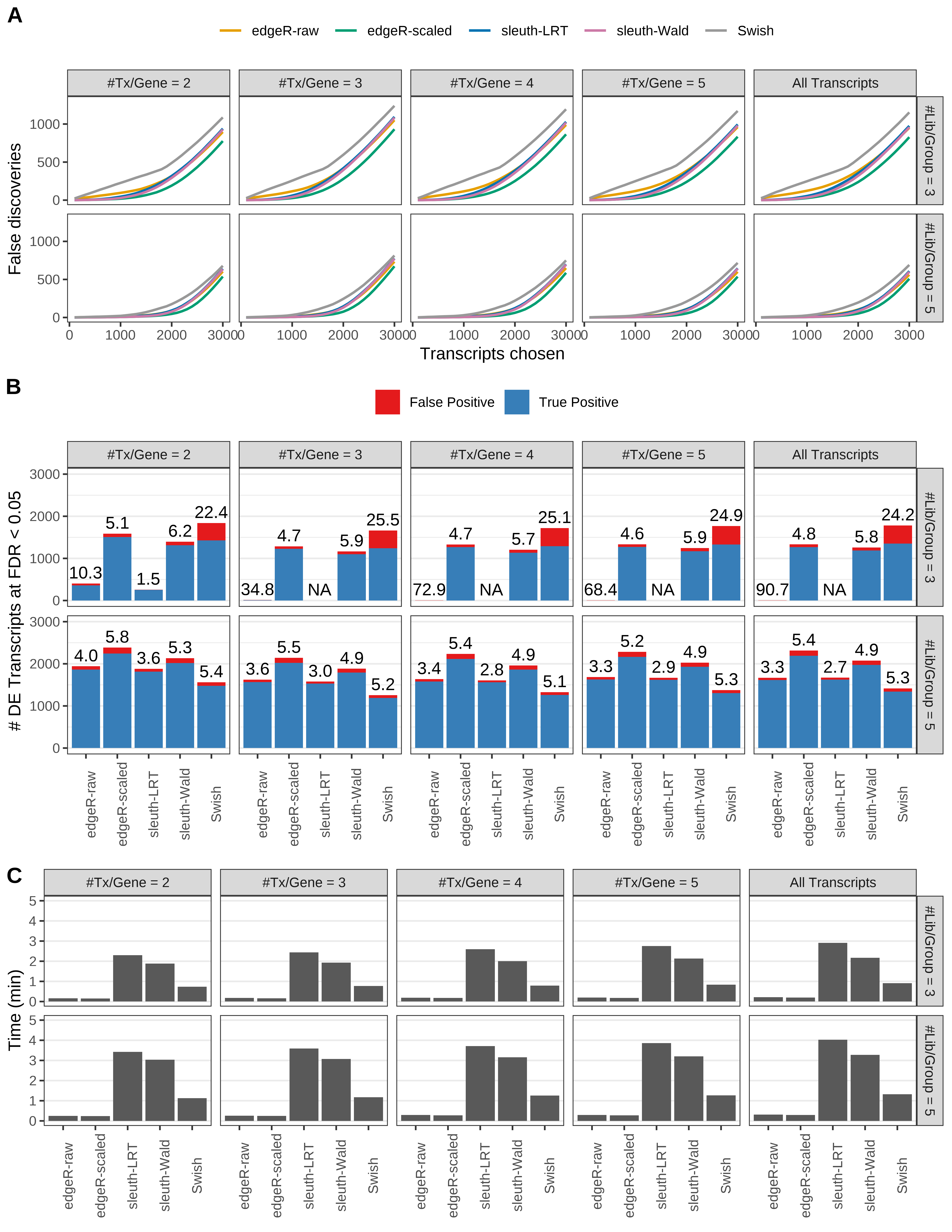
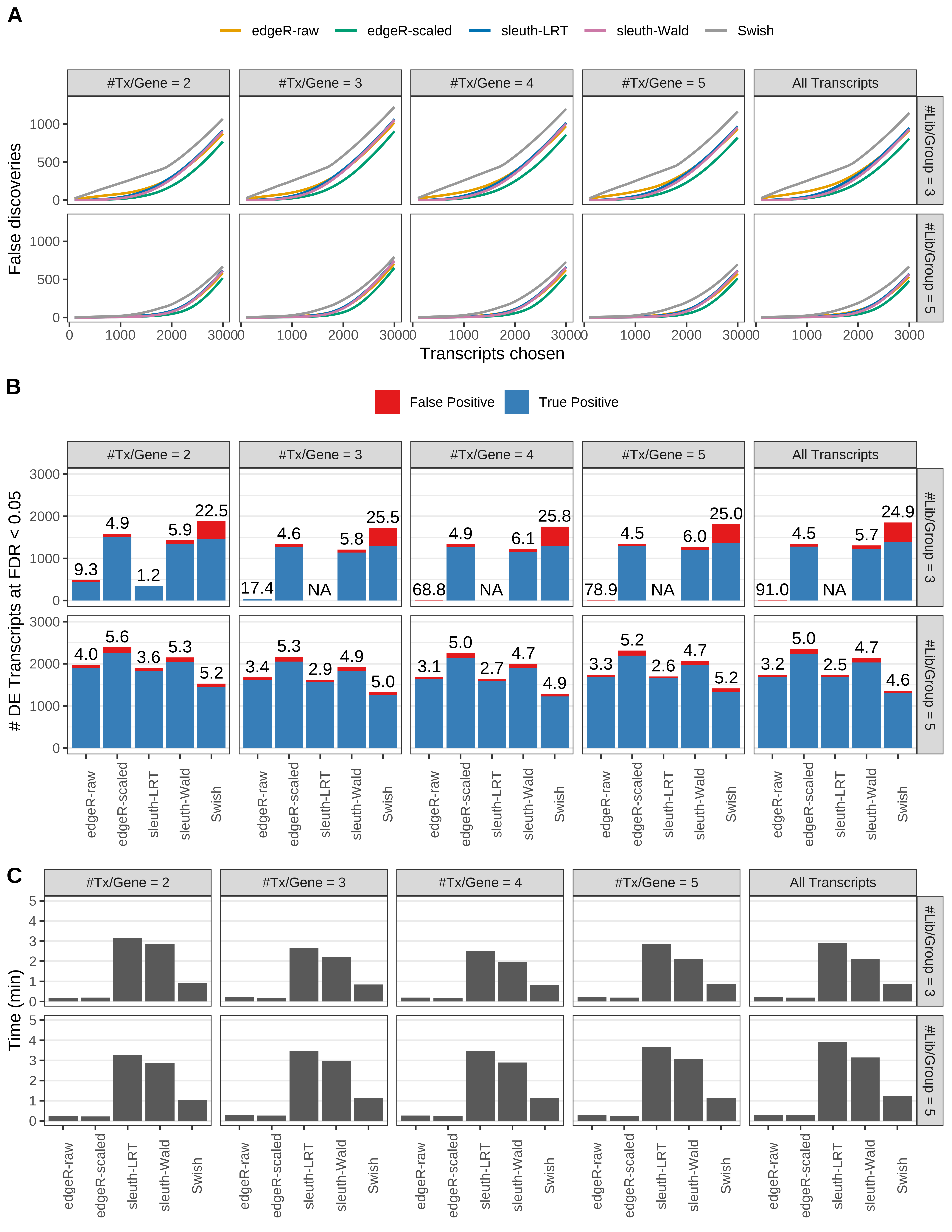
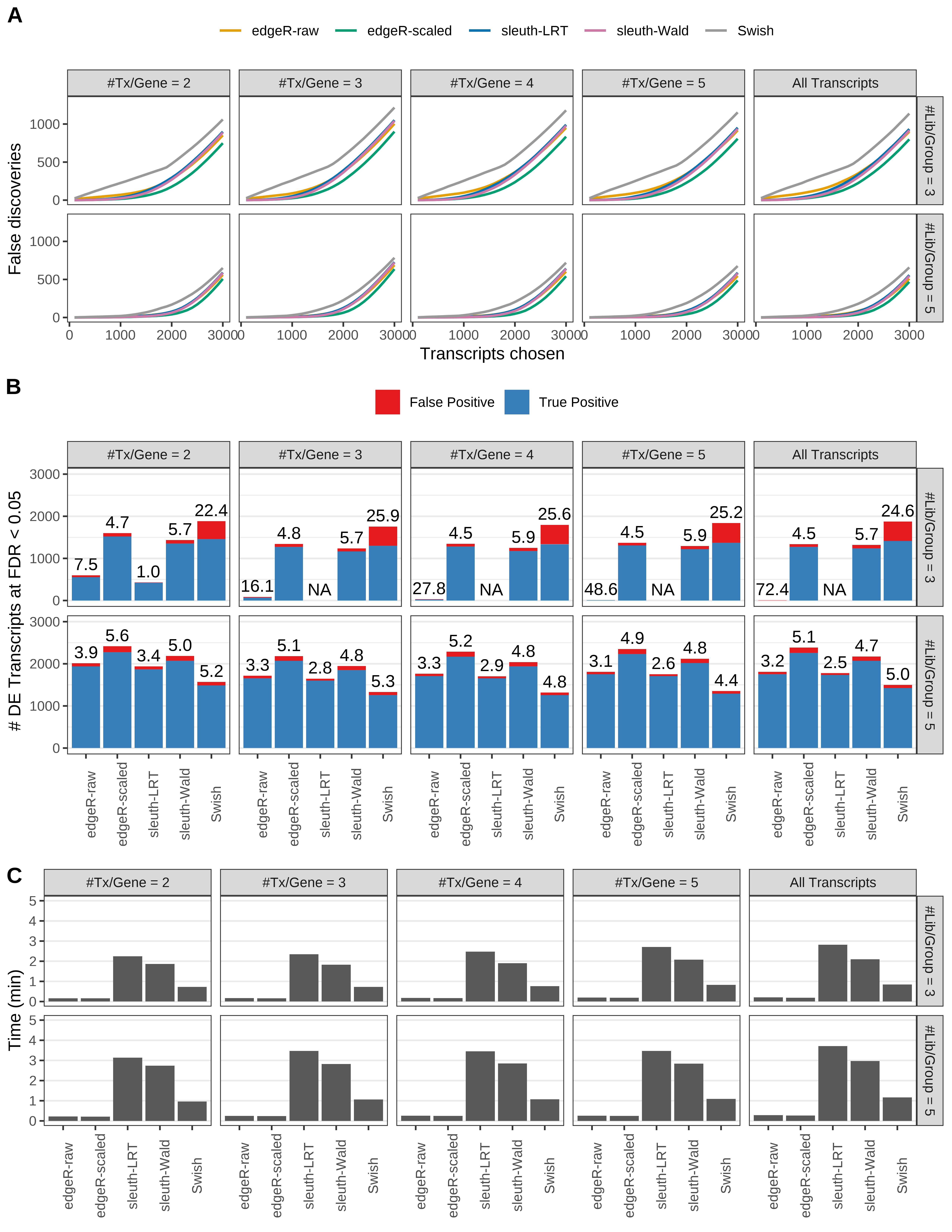
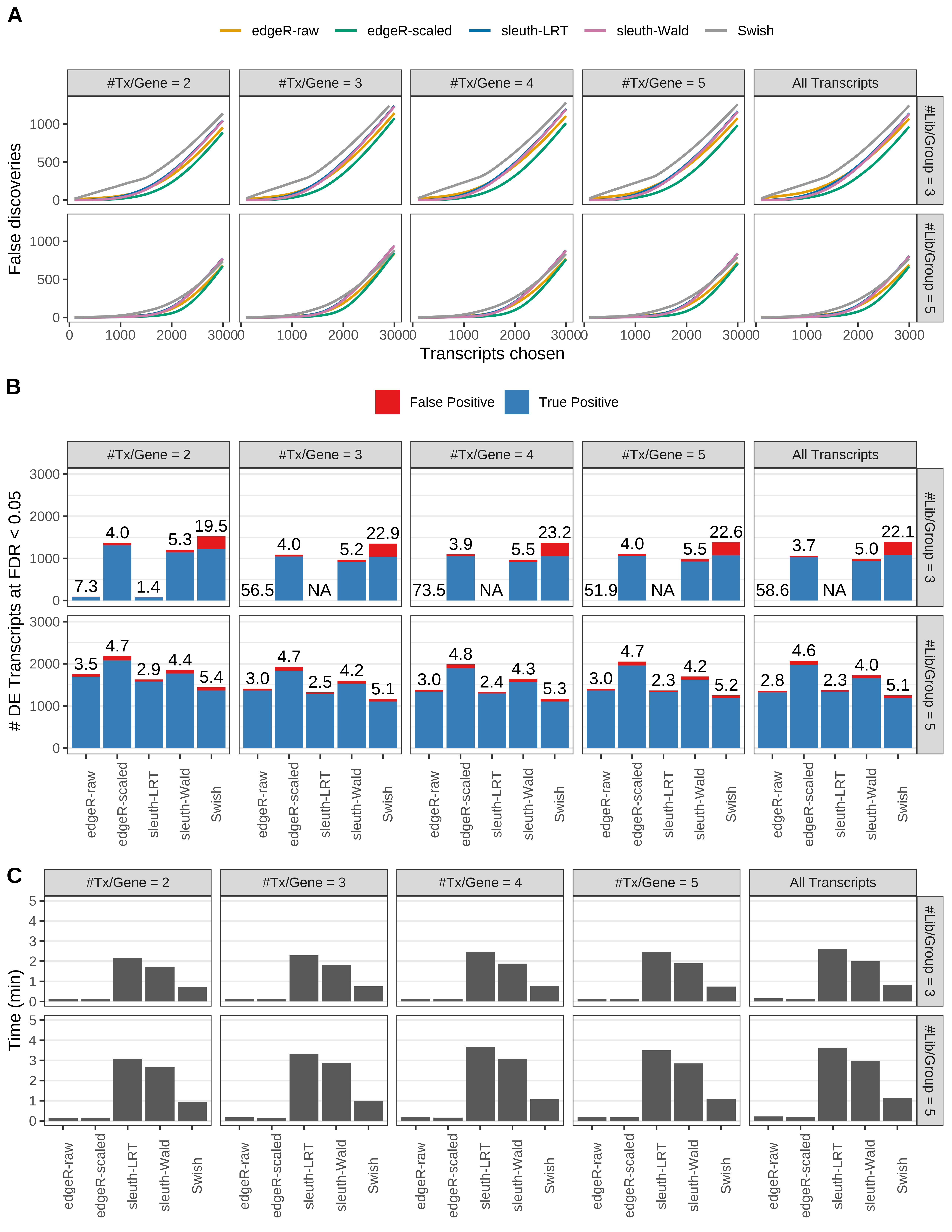
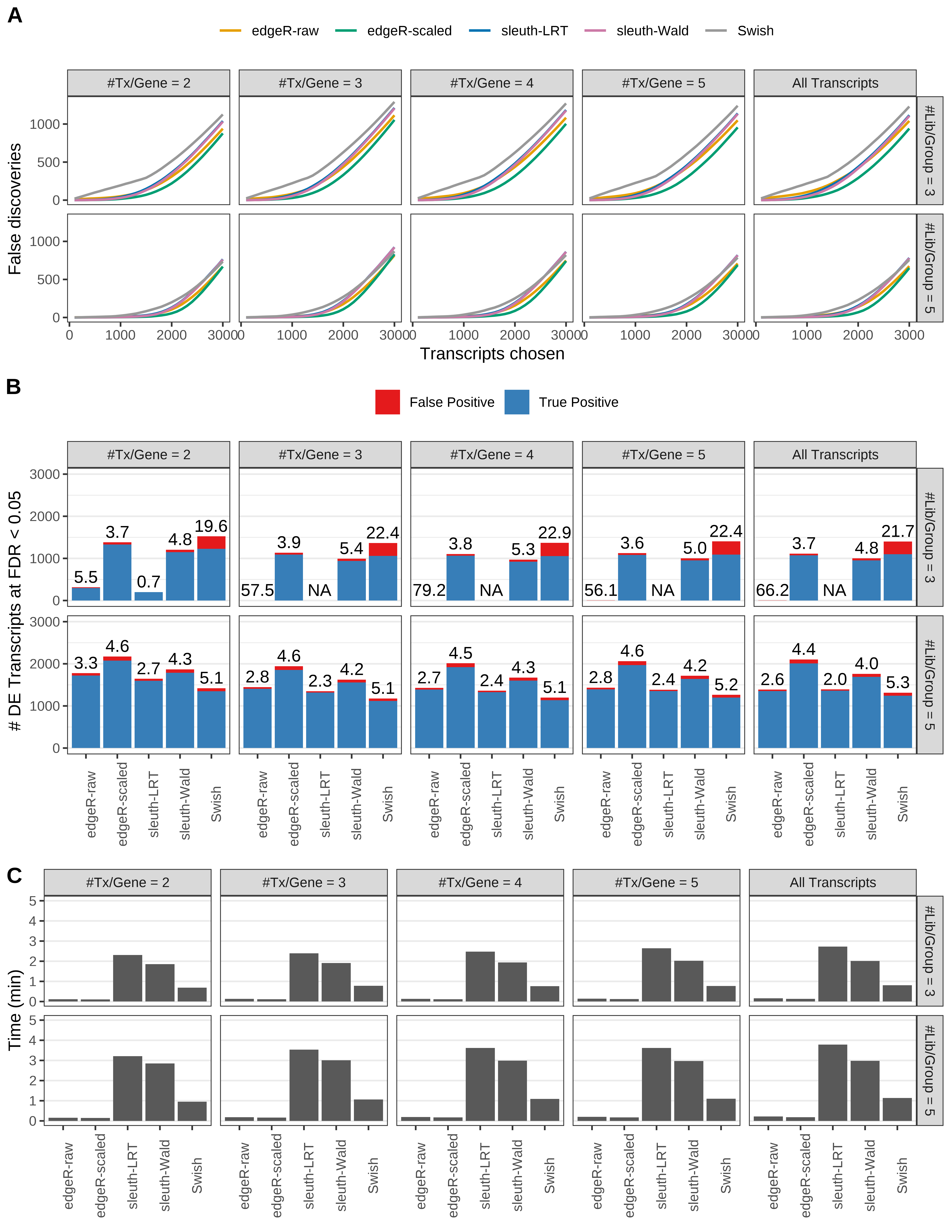
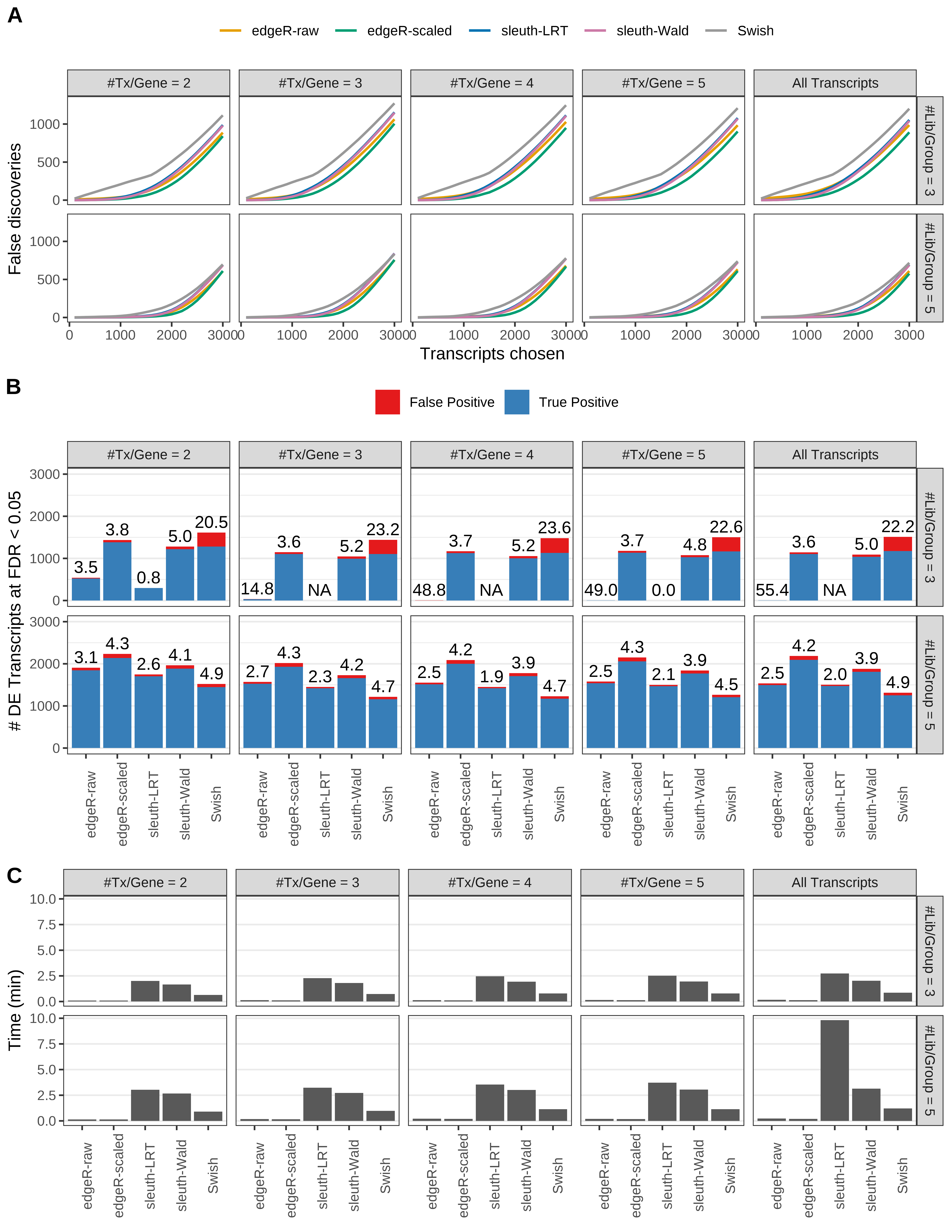
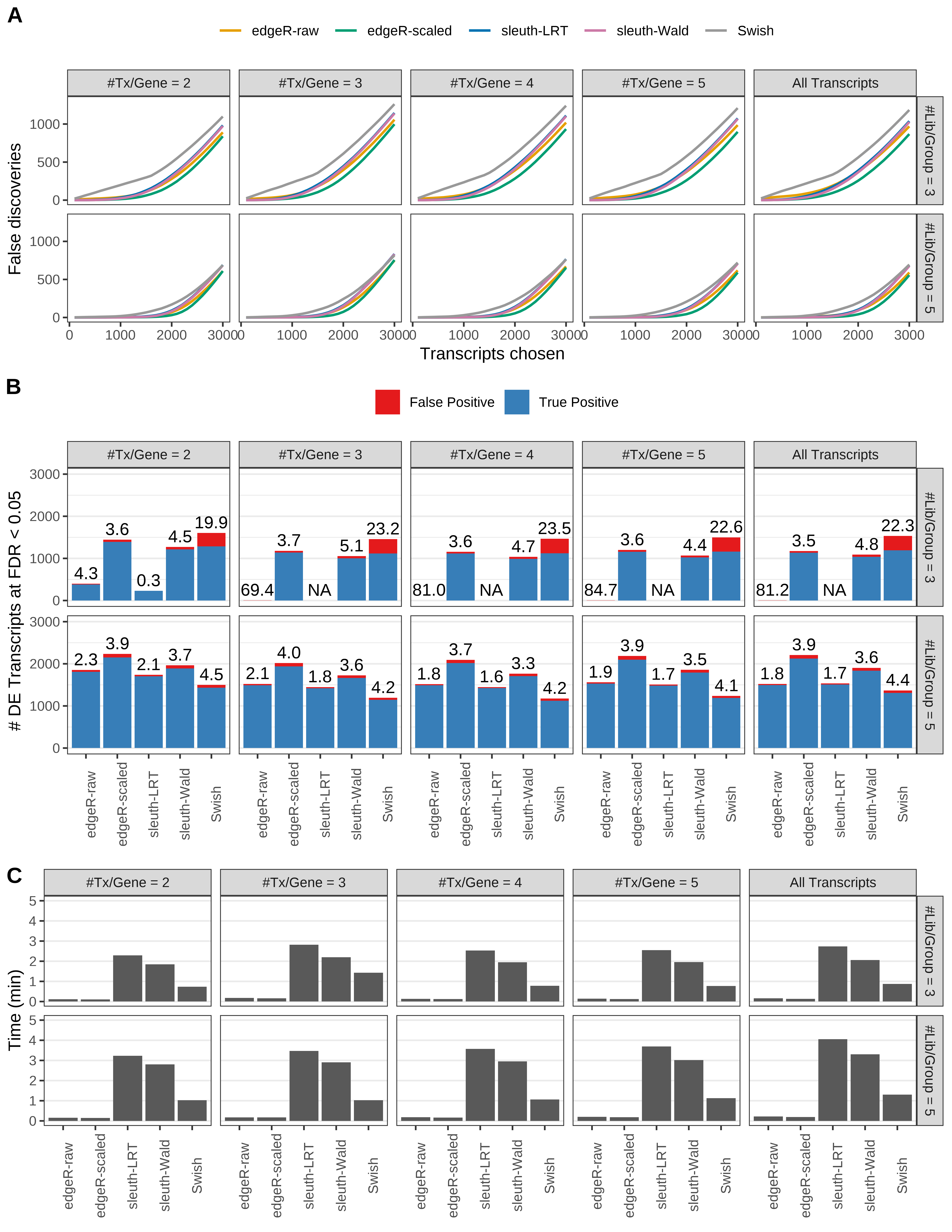
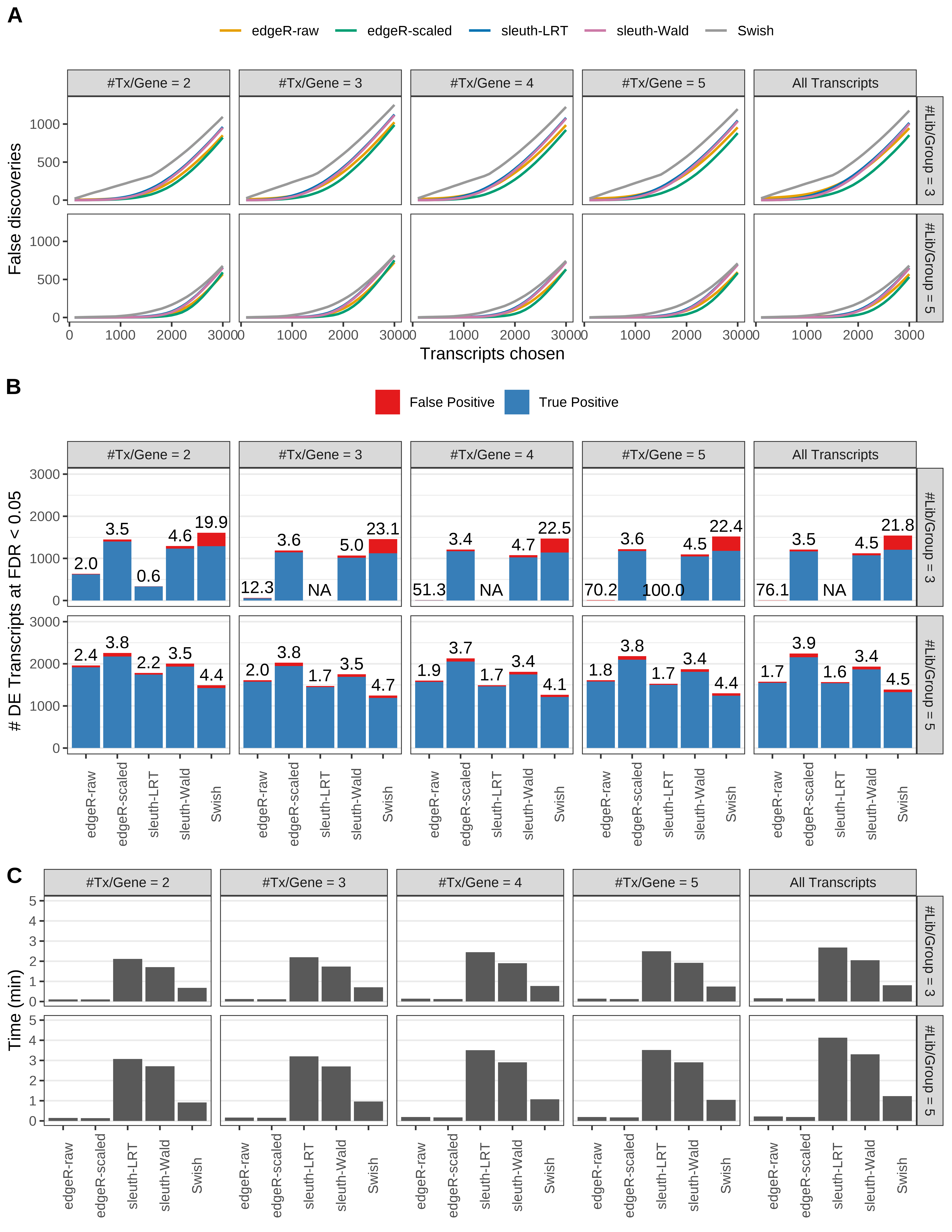
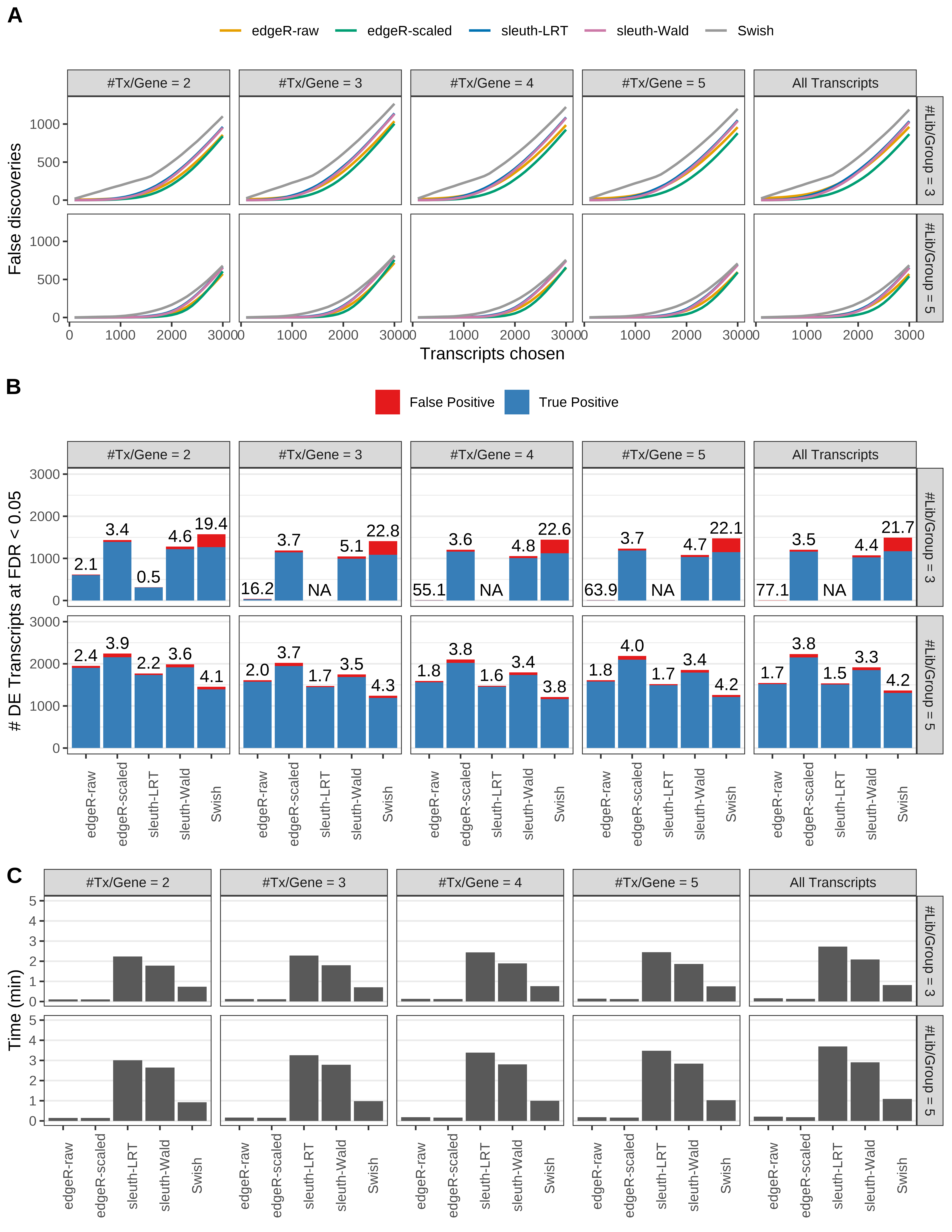
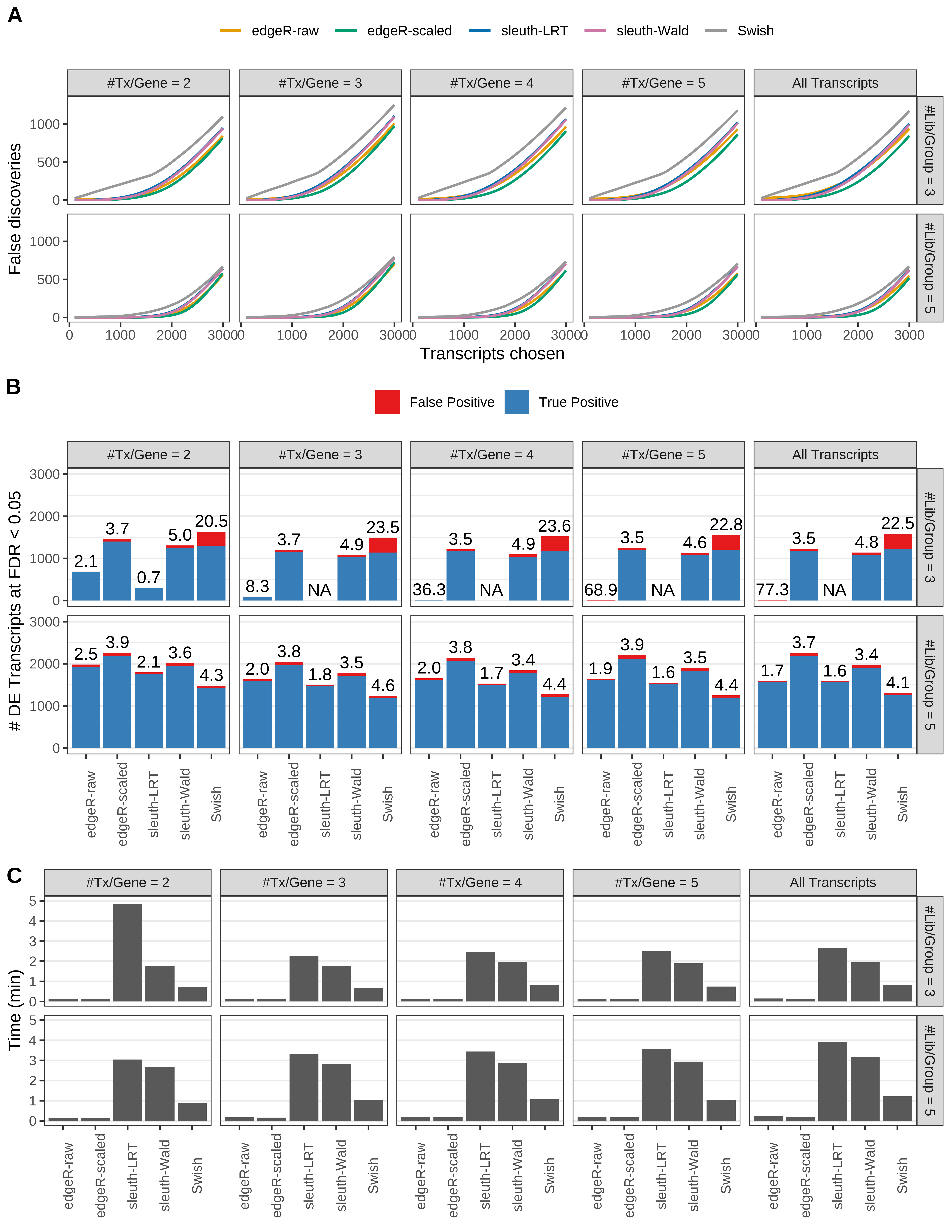
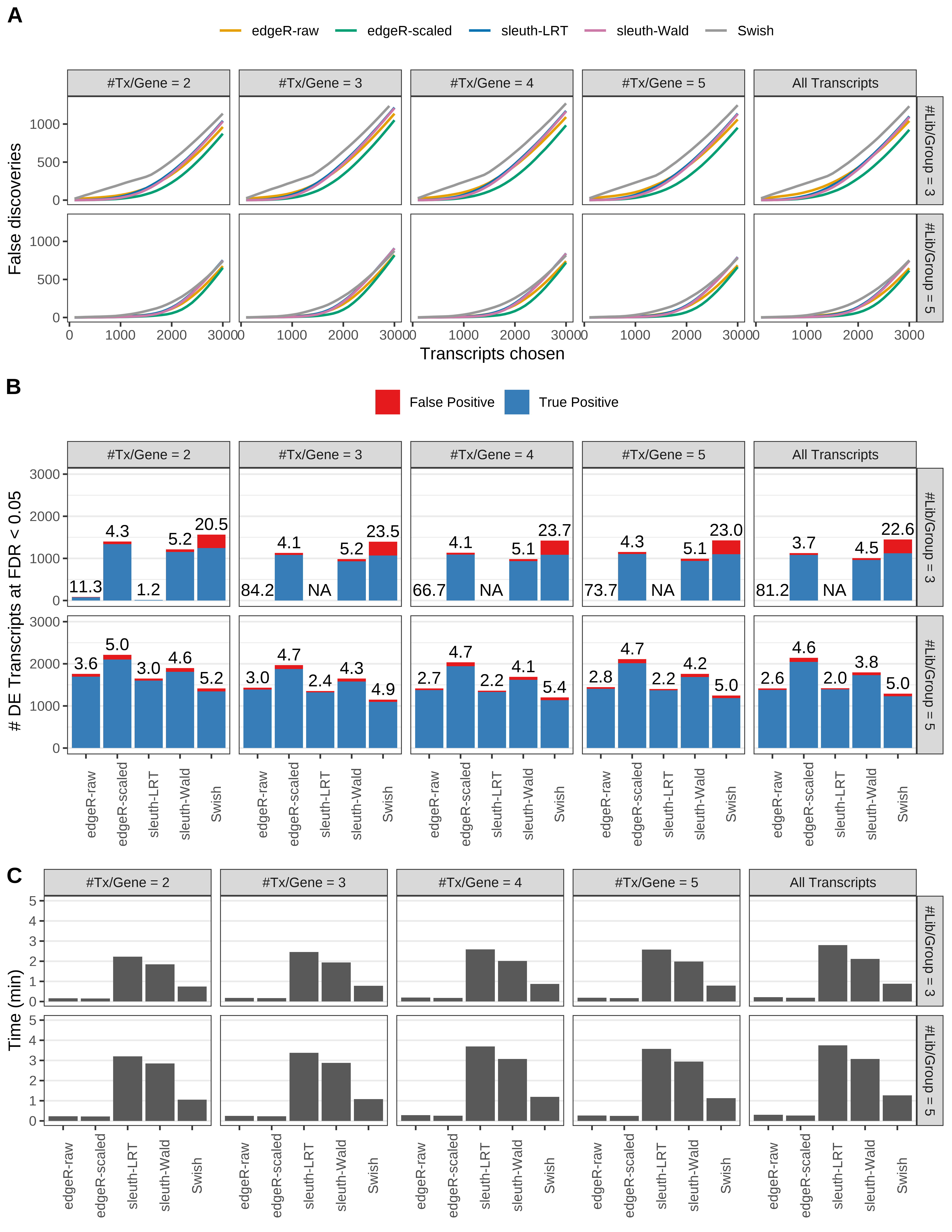
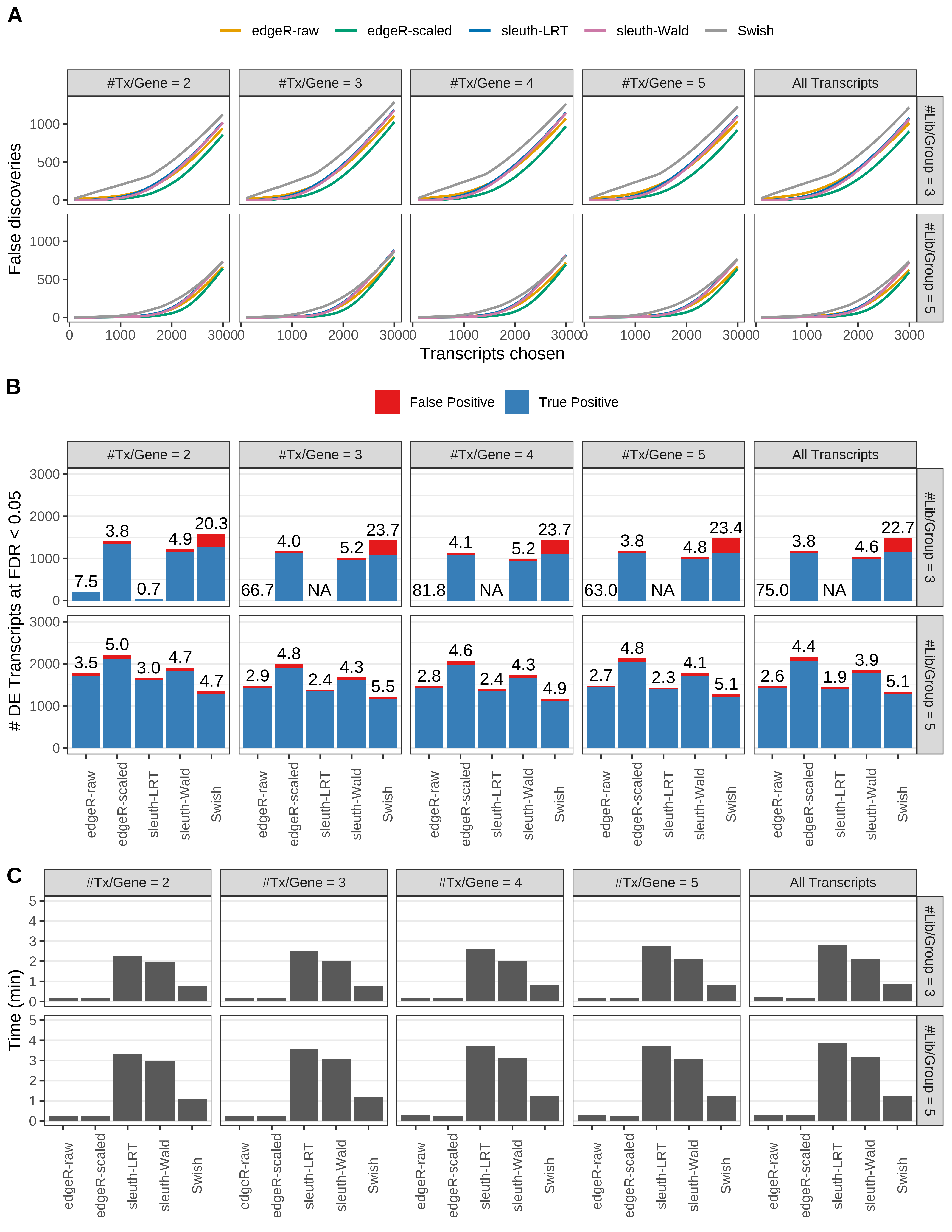
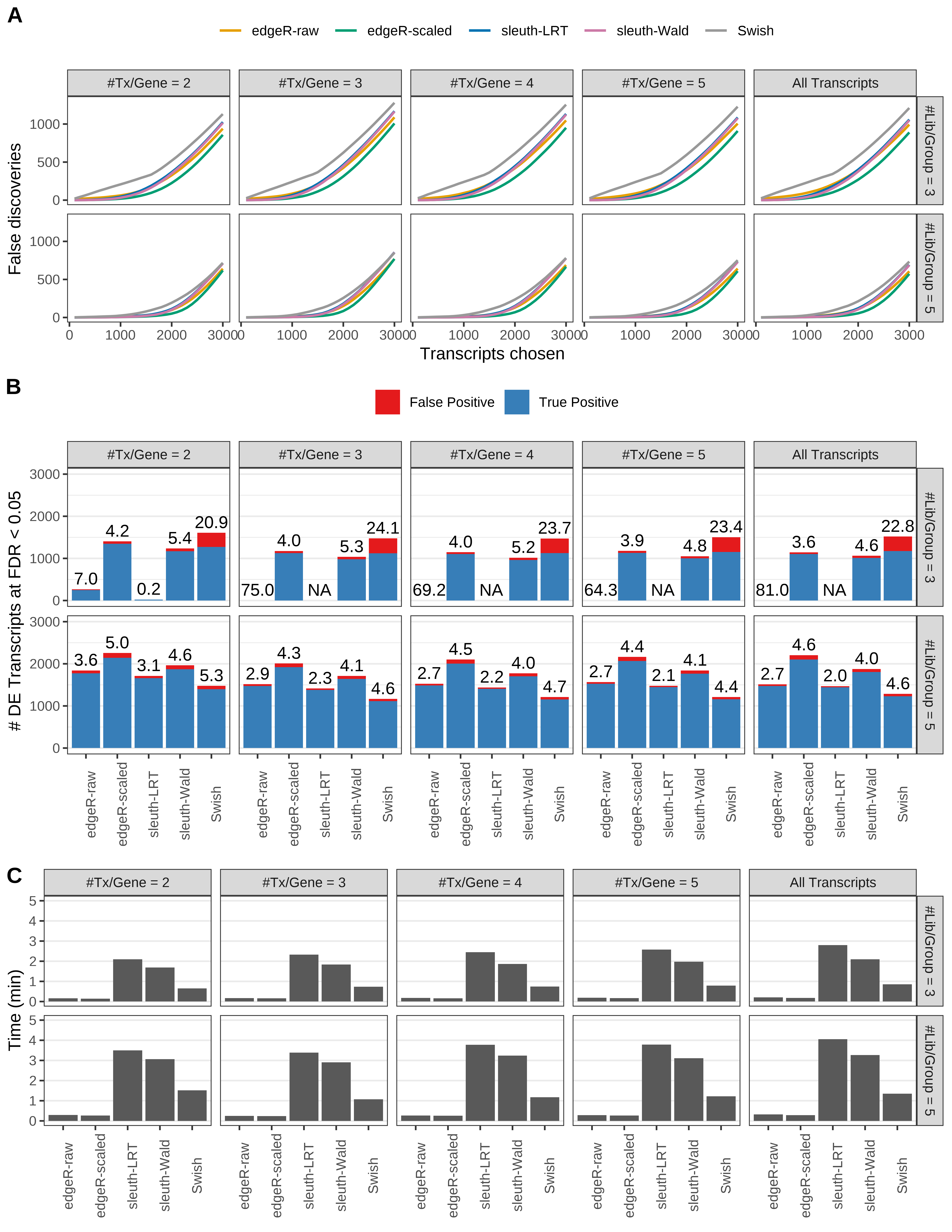
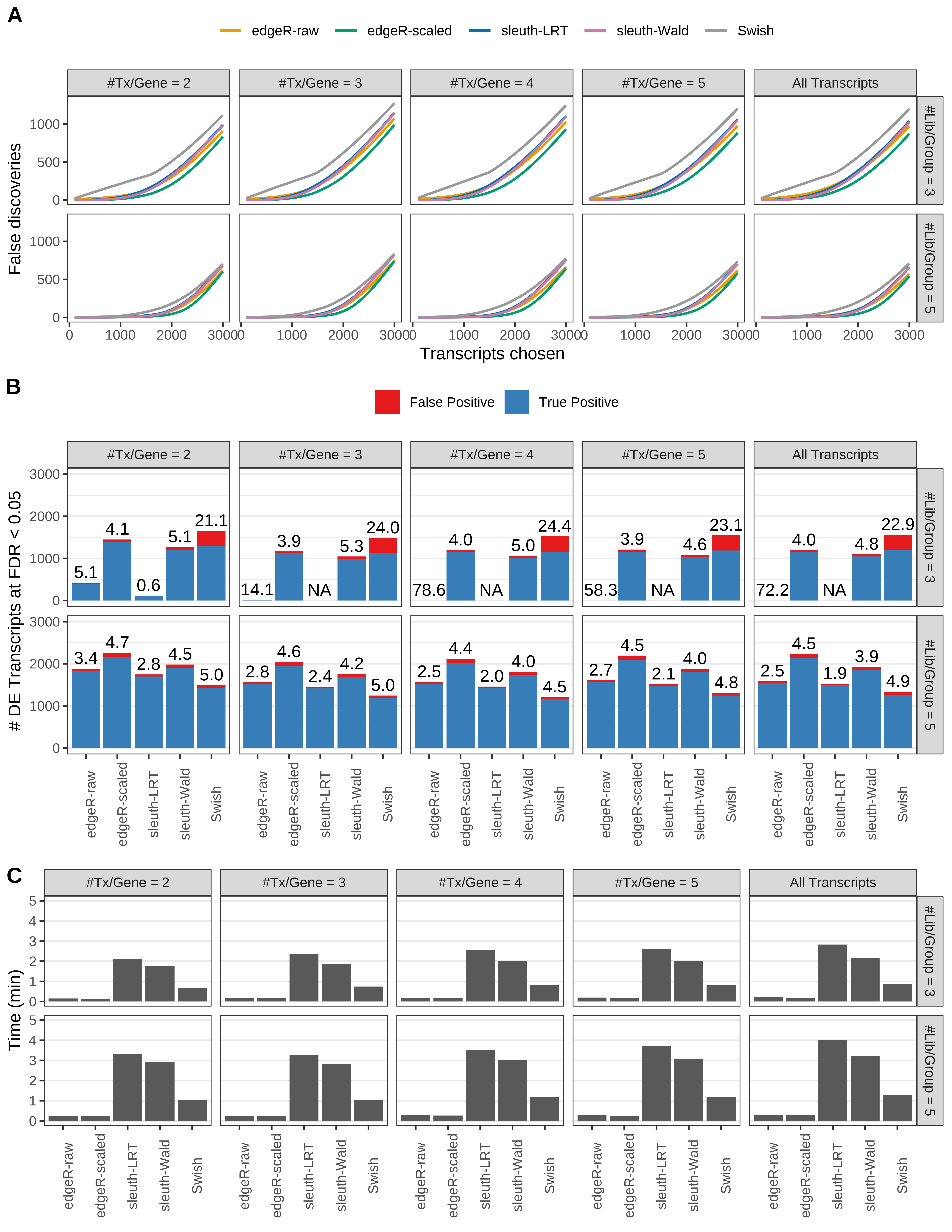
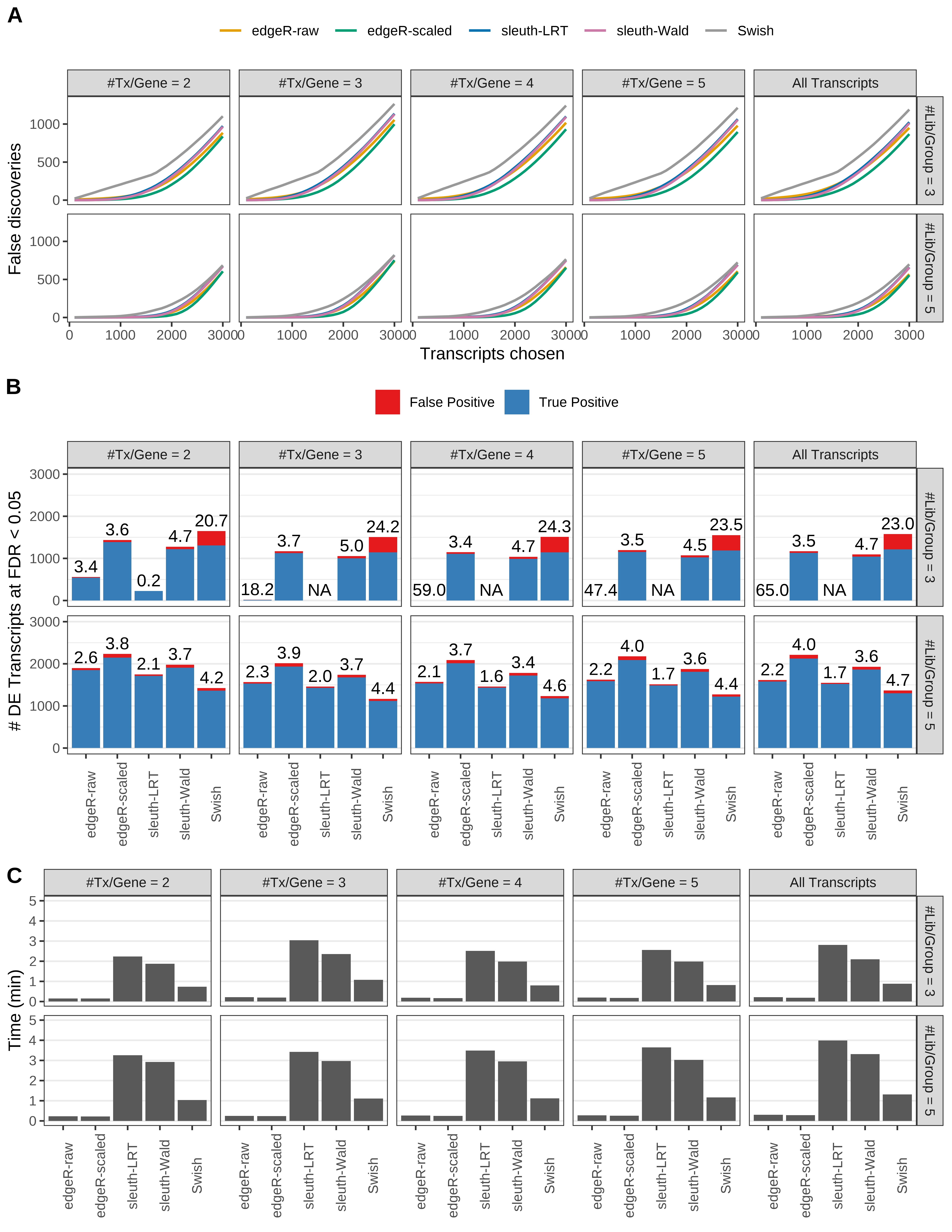
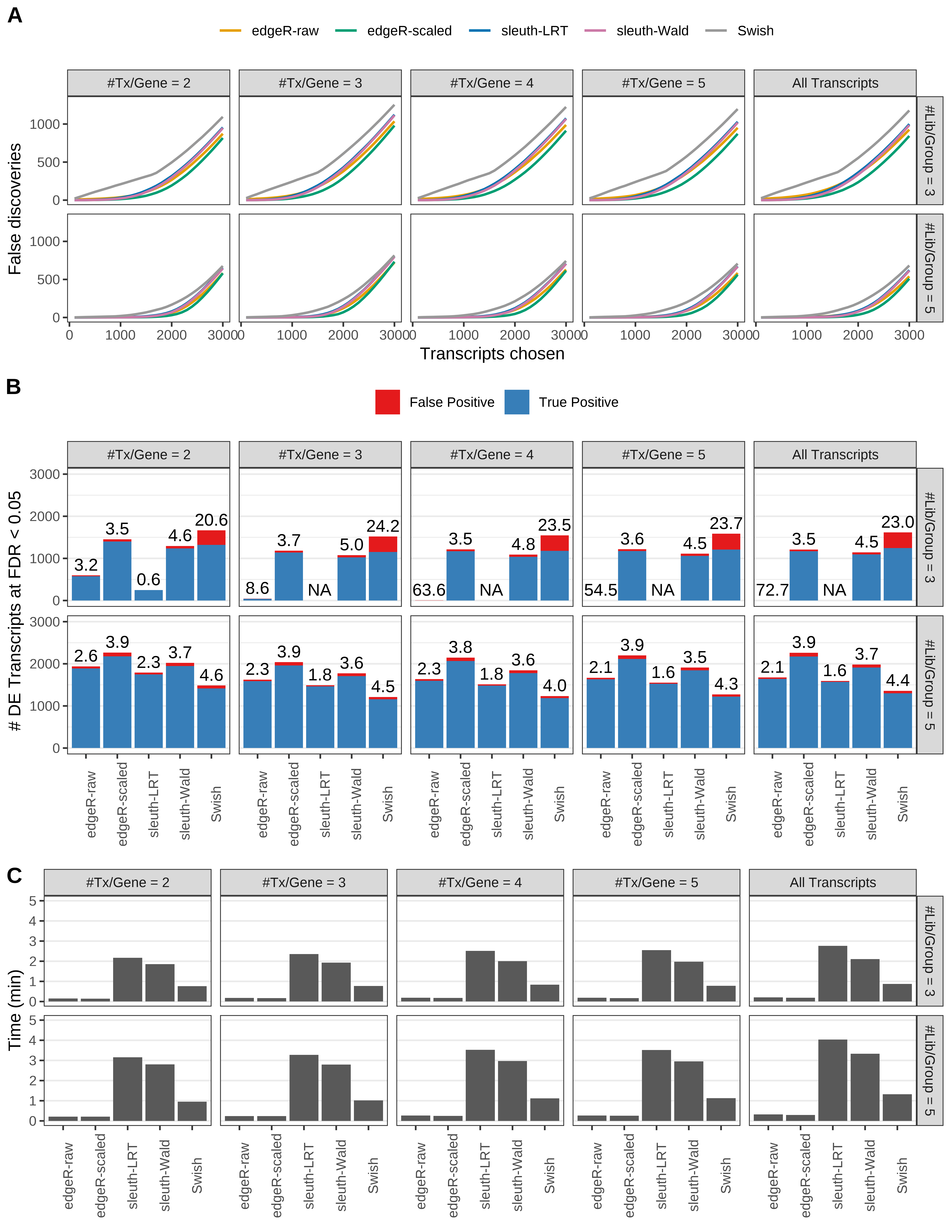
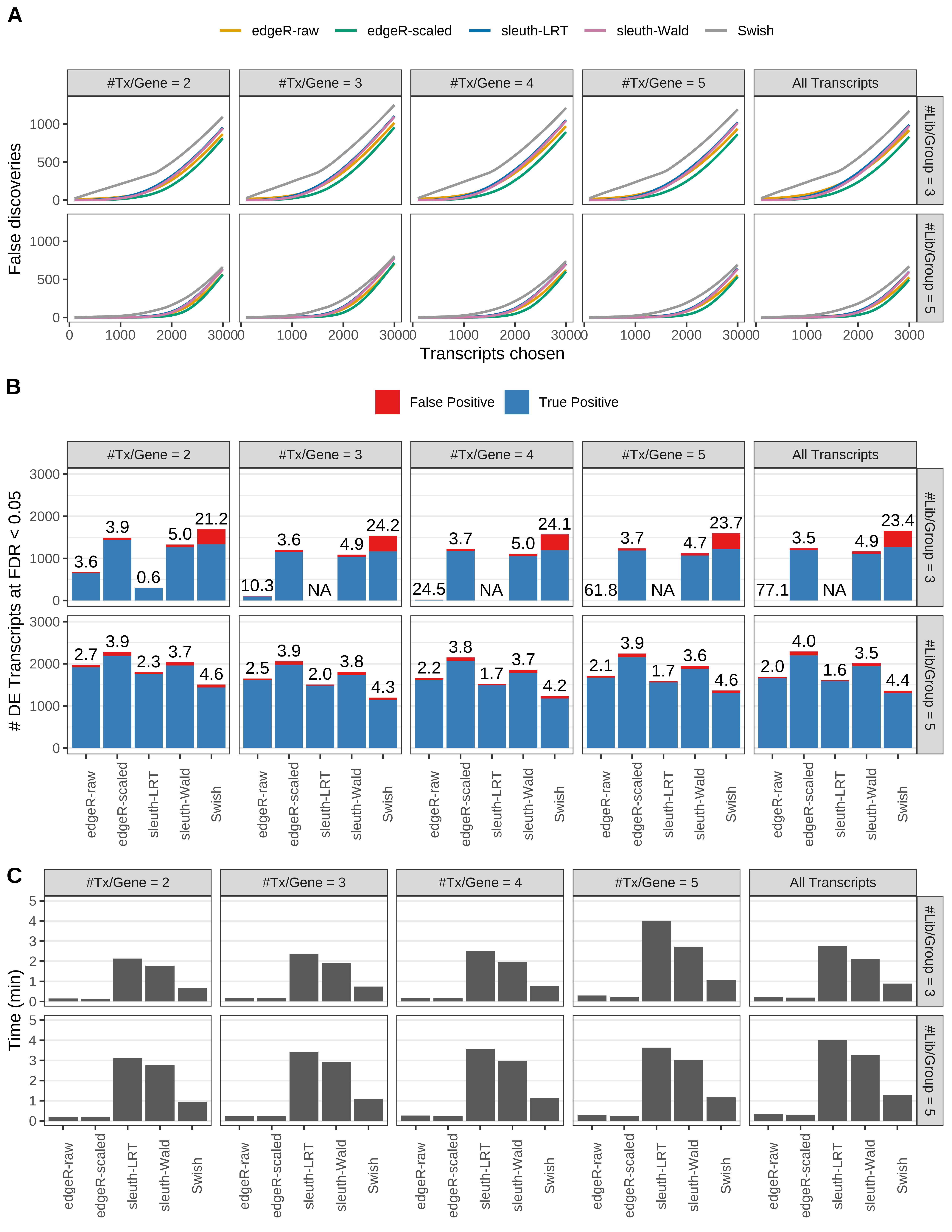
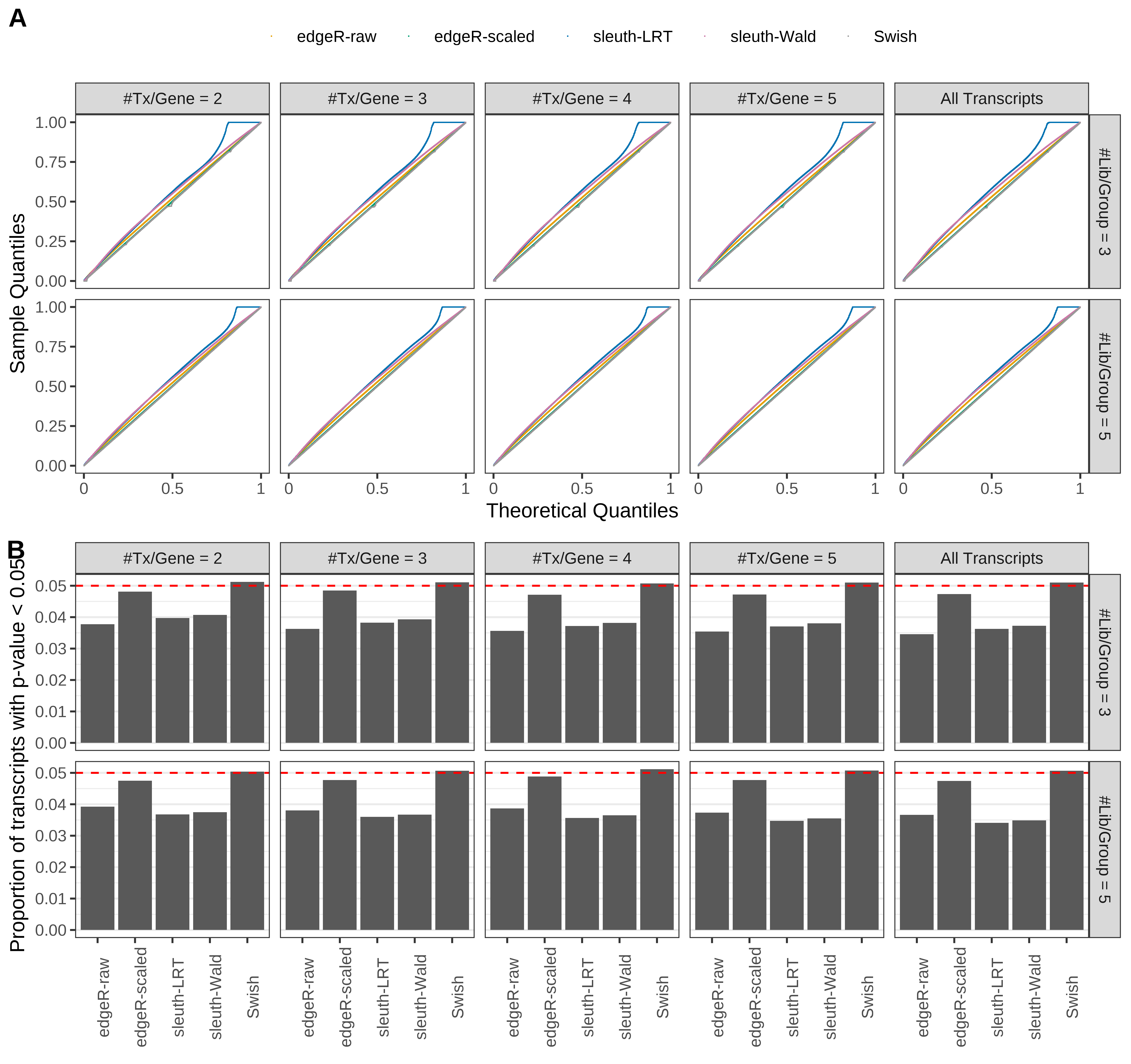
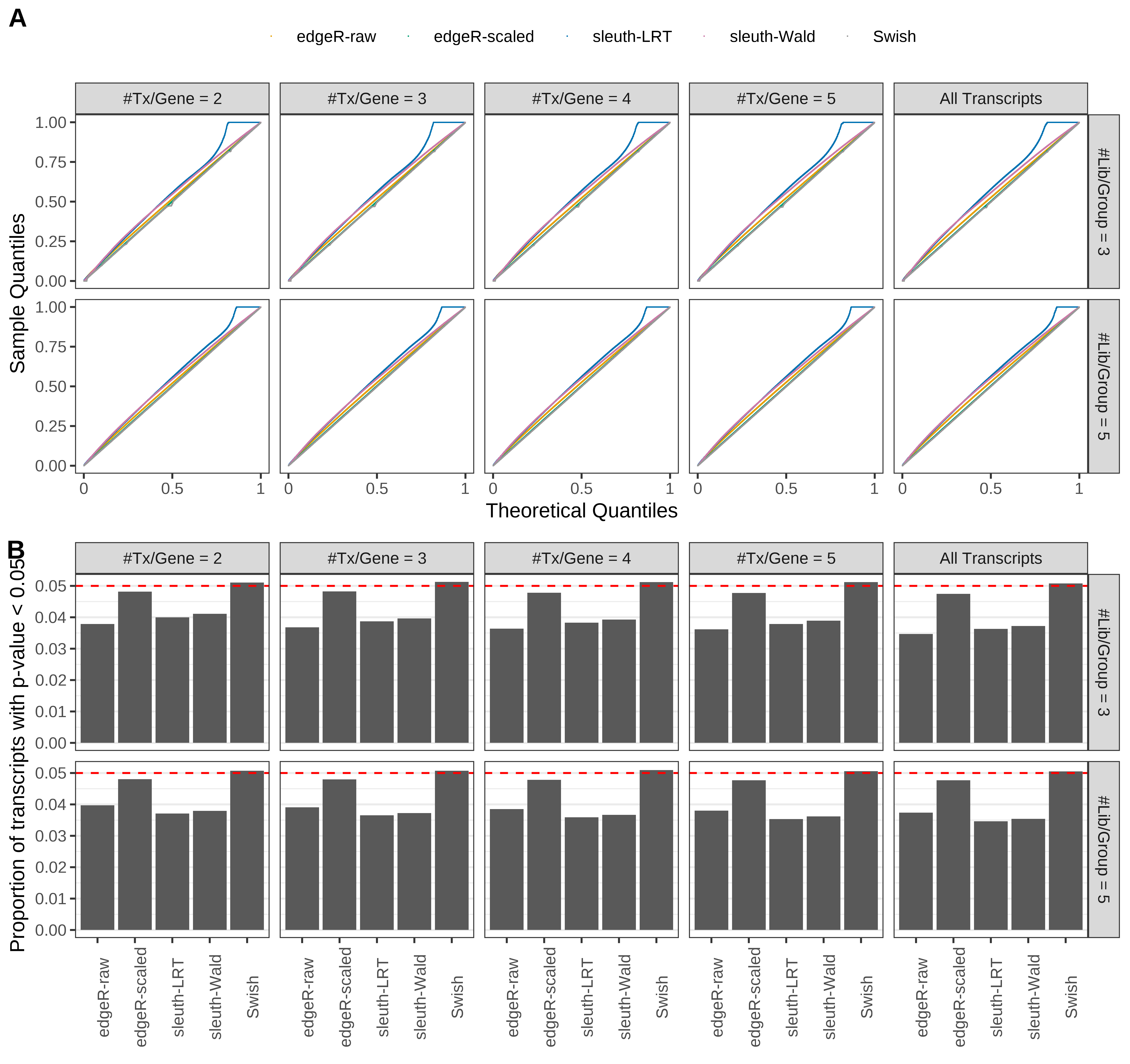
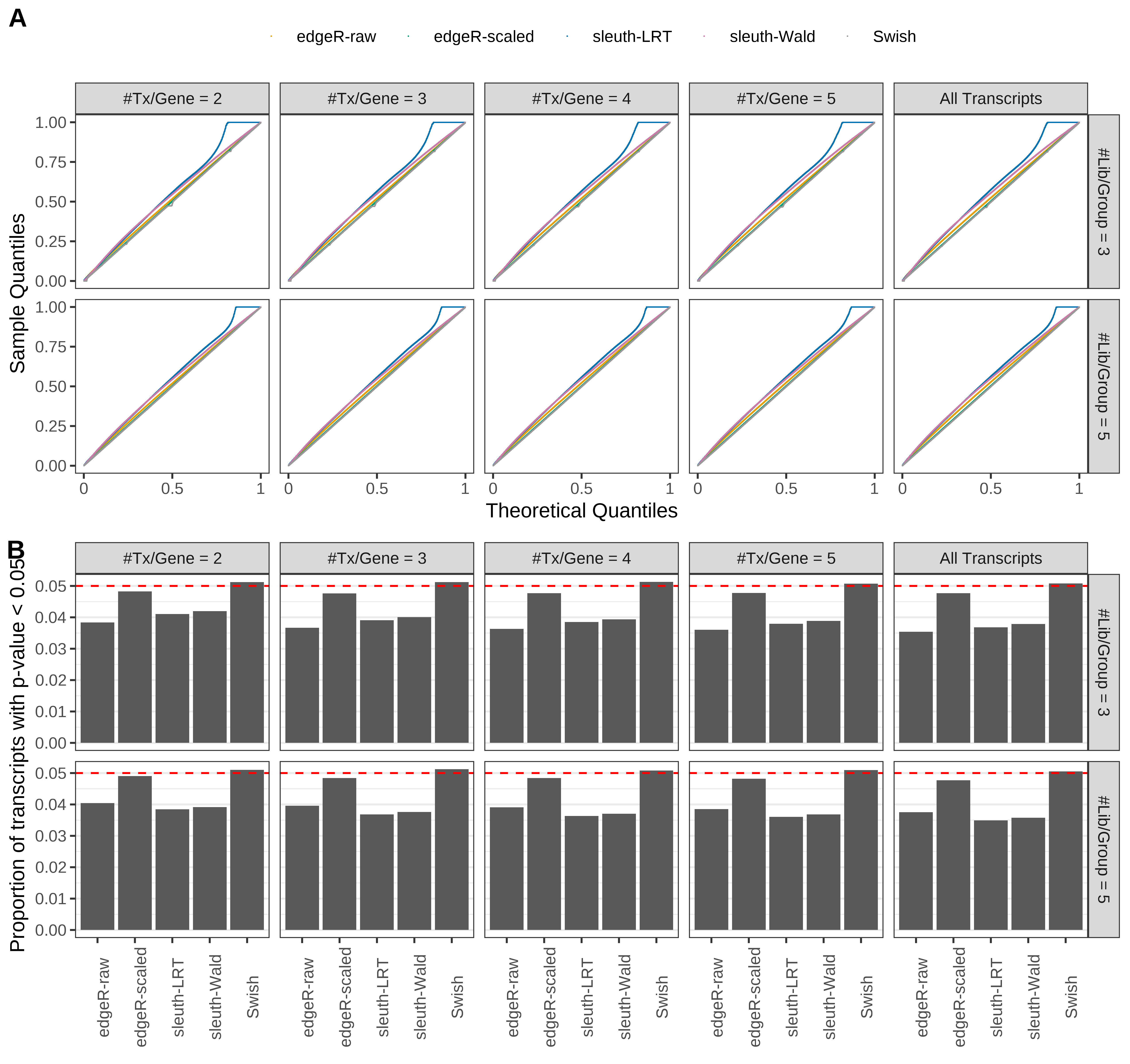
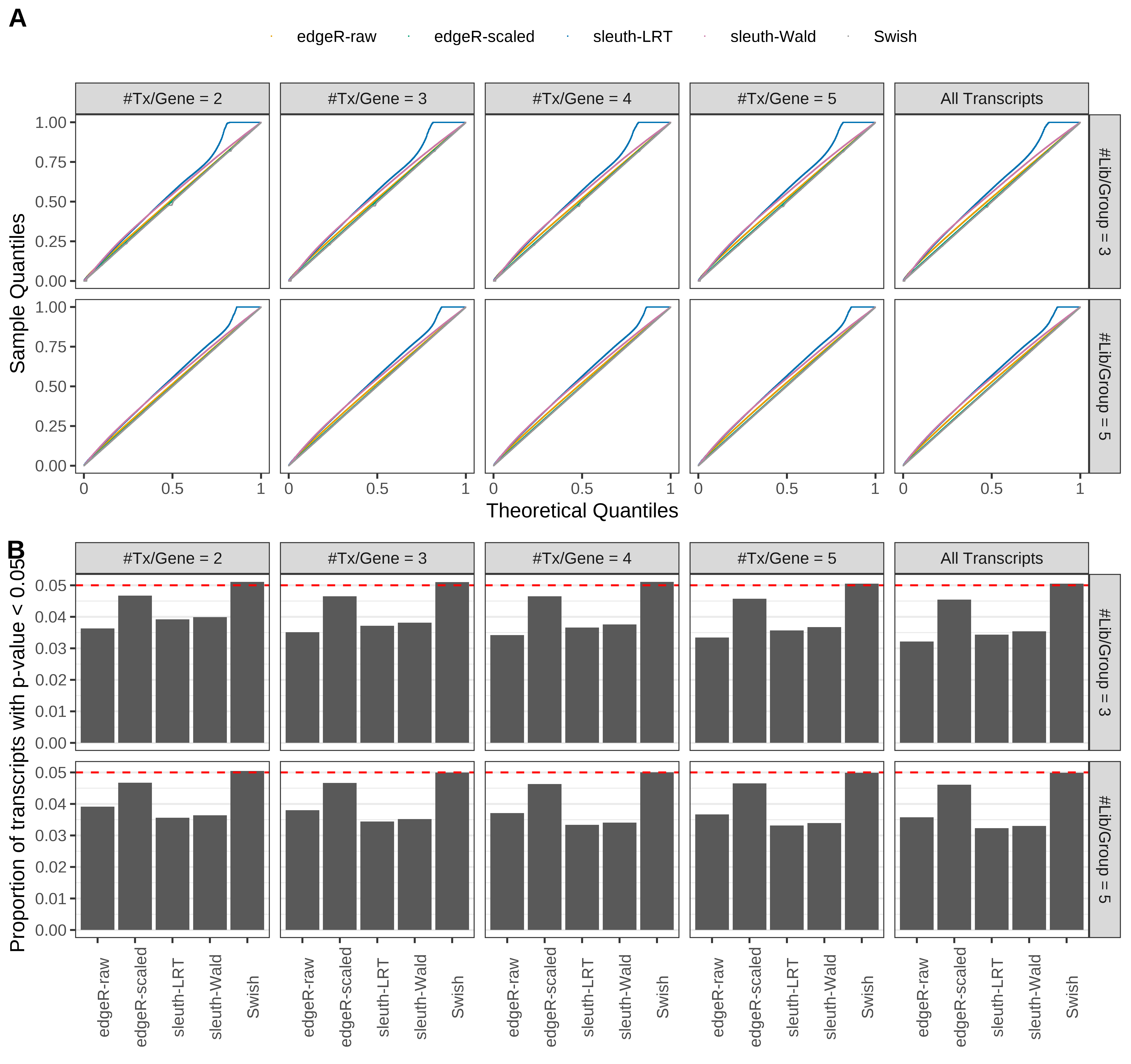
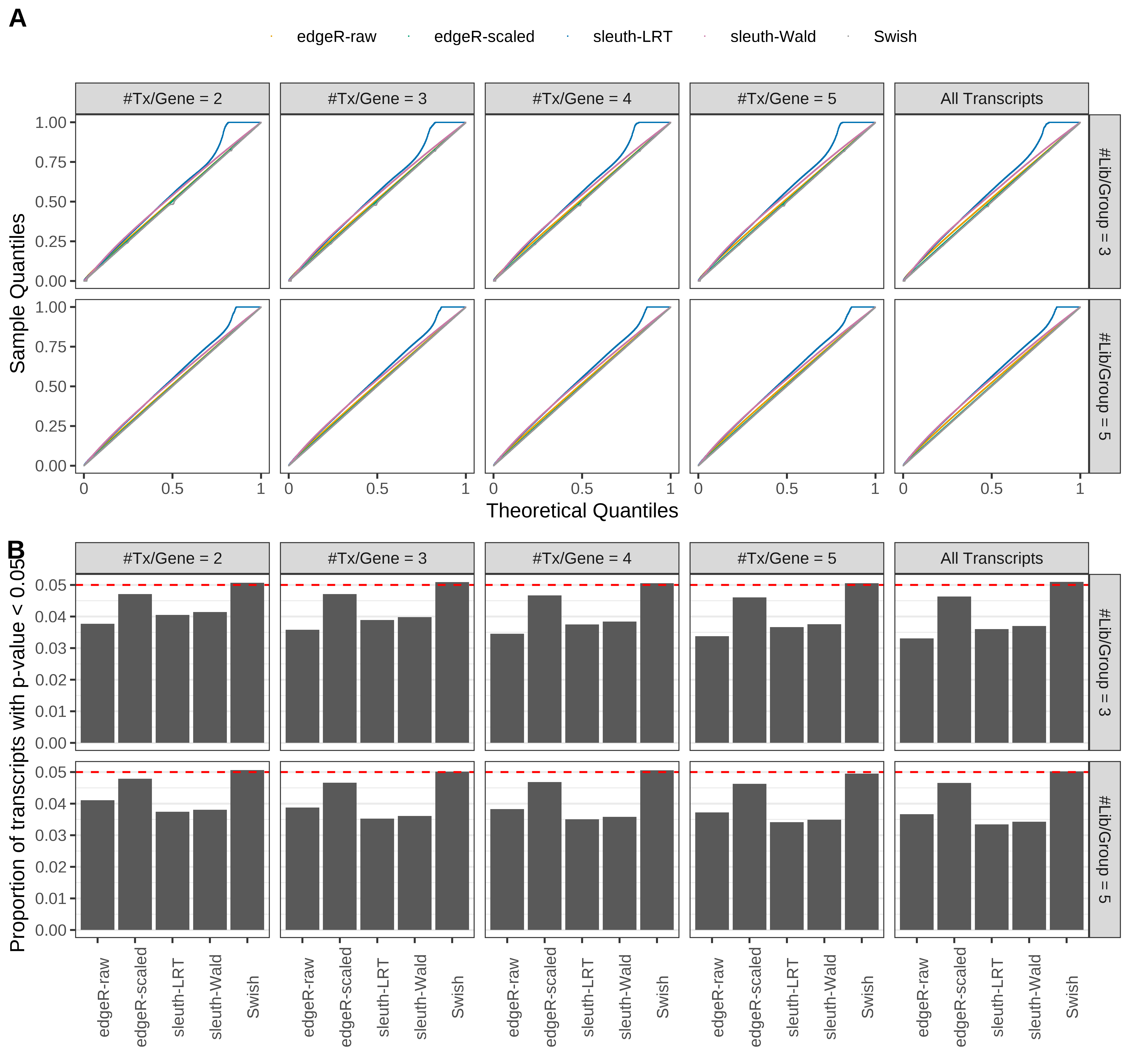
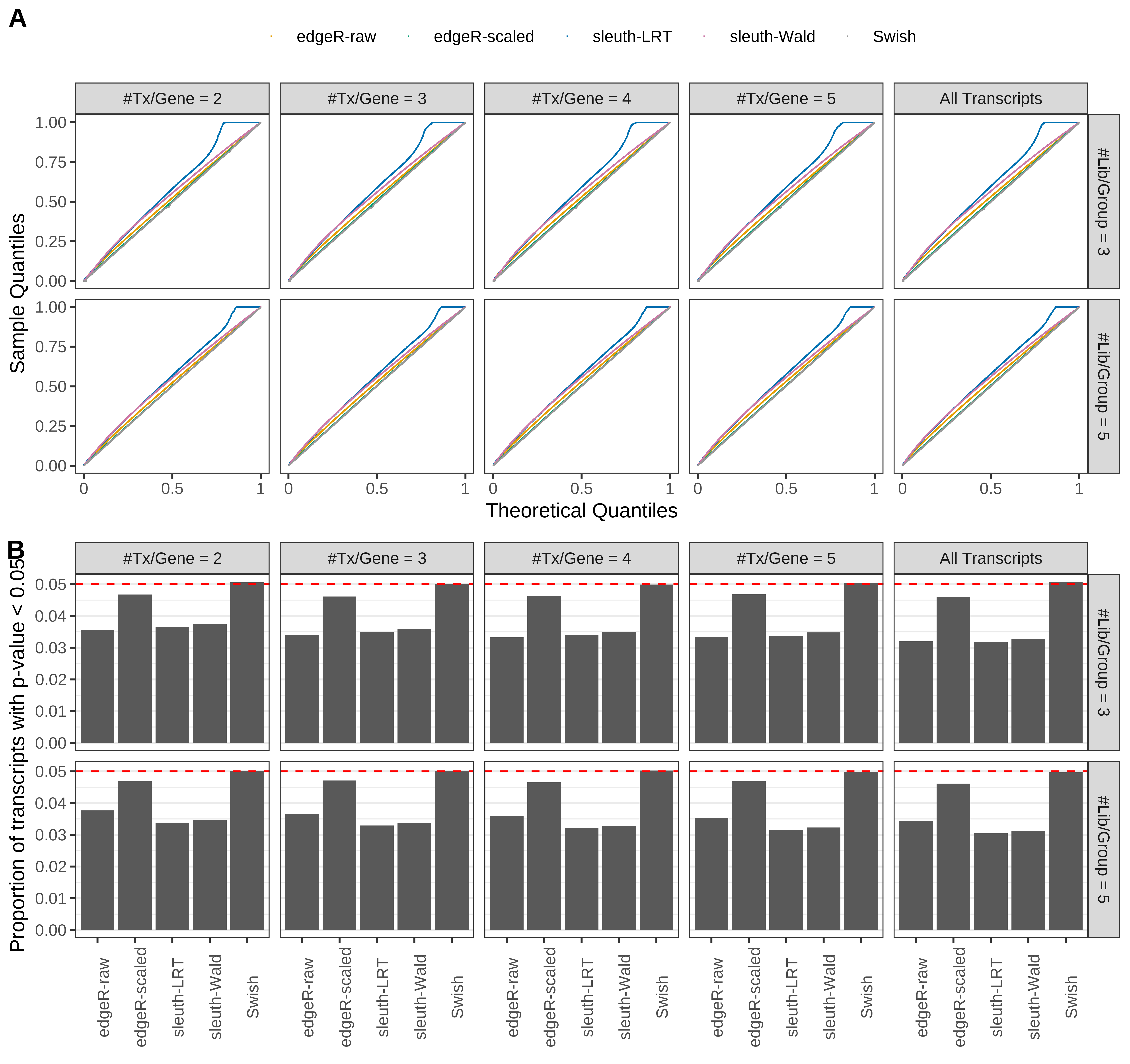
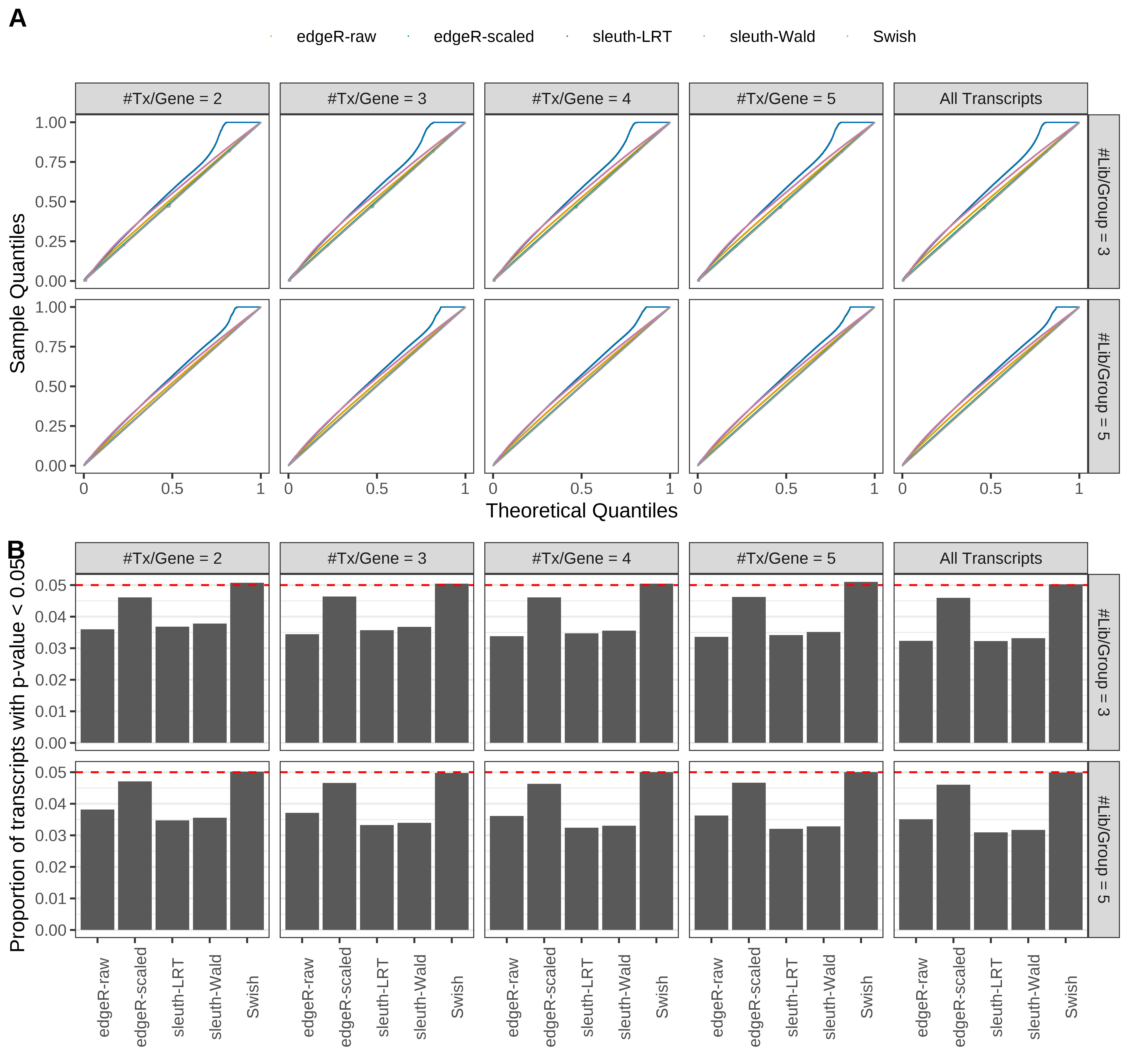
+ }The results of each simulation scenario are presented as a set of three figures. The first set of figures (set A in the chunk below) compares methods in regards to power (sensitivity), false discovery rate, and computing time. The second set of figures (set B in the chunk below) compares methods in regards to type 1 error rate control in a null simulation (i.e., a simulation without any truly differential expression between groups). The last and third set of figures (set C in the chunk below) compares methods in regards to the distribution of their unadjusted p-values in a null simulation.
> dt.scenario <- expand.grid('genome' = 'mm39',
+                            'length' = c('50bp','75bp','100bp','125bp','150bp'),
+                            'read' = c('single-end','paired-end'),
+                            'quantifier' = c('Salmon','kallisto'),
+                            'scenario' = c('balanced','unbalanced'),
+                            stringsAsFactors = FALSE)
>
> plots <- lapply(seq_len(nrow(dt.scenario)),function(i){
+   scenario <- as.character(dt.scenario[i,])
+   names(scenario) <- colnames(dt.scenario)
+
+   figA <-
+     list(plotFDRCurve(x = subsetDT(dt.fdr,scenario,'A'),3000),
+          plotPowerBars(x = subsetDT(dt.metrics,scenario,'A'),0.05,3000),
+          plotTime(x = subsetDT(dt.time,scenario,'A')))
+
+   figB <-
+     list(plotQQPlot(x = subsetDT(dt.quantile,scenario,'B')),
+          plotType1Error(x = subsetDT(dt.metrics,scenario,'B'),0.05))
+
+   figC <-
+     list(plotPValues(x = subsetDT(dt.pvalue,scenario,'C','#Tx/Gene = 2')),
+          plotPValues(x = subsetDT(dt.pvalue,scenario,'C','#Tx/Gene = 3')),
+          plotPValues(x = subsetDT(dt.pvalue,scenario,'C','#Tx/Gene = 4')),
+          plotPValues(x = subsetDT(dt.pvalue,scenario,'C','#Tx/Gene = 5')),
+          plotPValues(x = subsetDT(dt.pvalue,scenario,'C','All Transcripts')))
+
+   figC <- lapply(seq_along(figC),cleanPlot,fig = figC)
+
+   out <-
+     list('scenario' = scenario,
+          'panelA' = ggarrange(plotlist = figA,nrow = 3,labels = c('A','B','C'),
+                               heights = c(0.95,1.25,0.95)),
+          'panelB' = ggarrange(plotlist = figB,nrow = 2,labels = c('A','B')),
+          'panelC' = ggarrange(plotlist = figC,nrow = 5,
+                               labels = c('A','B','C','D','E'),
+                               heights = c(1,0.95,0.95,0.95,1.25)))
+
+   return(out)
+ })
Below are the captions from each plot.
> cap <- paste0('Simulation results. Scenario with ',dt.scenario$genome,' genome, ',
+ dt.scenario$length,' ',dt.scenario$read,' reads quantified with ',
+ dt.scenario$quantifier,', and ',dt.scenario$scenario,' libraries.')
>
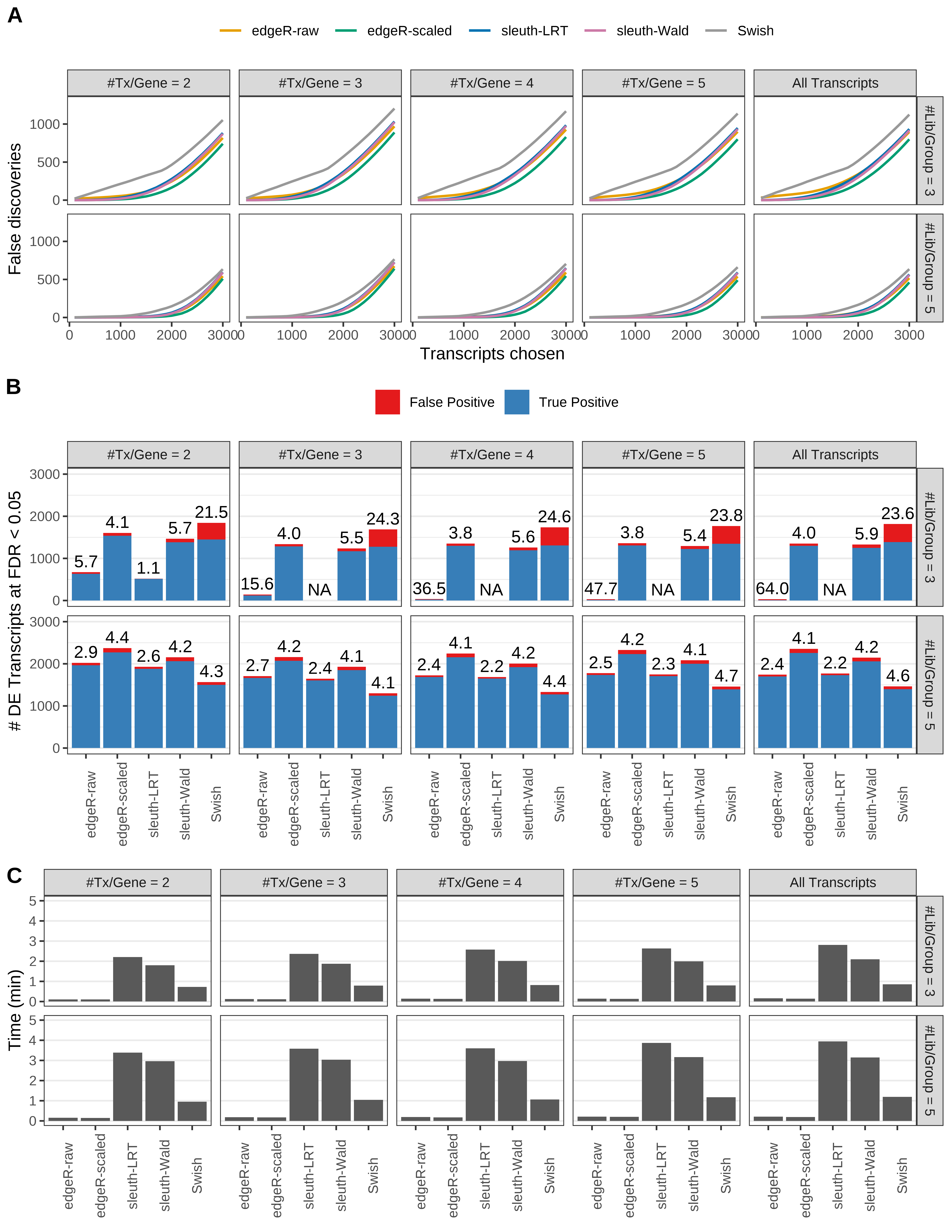
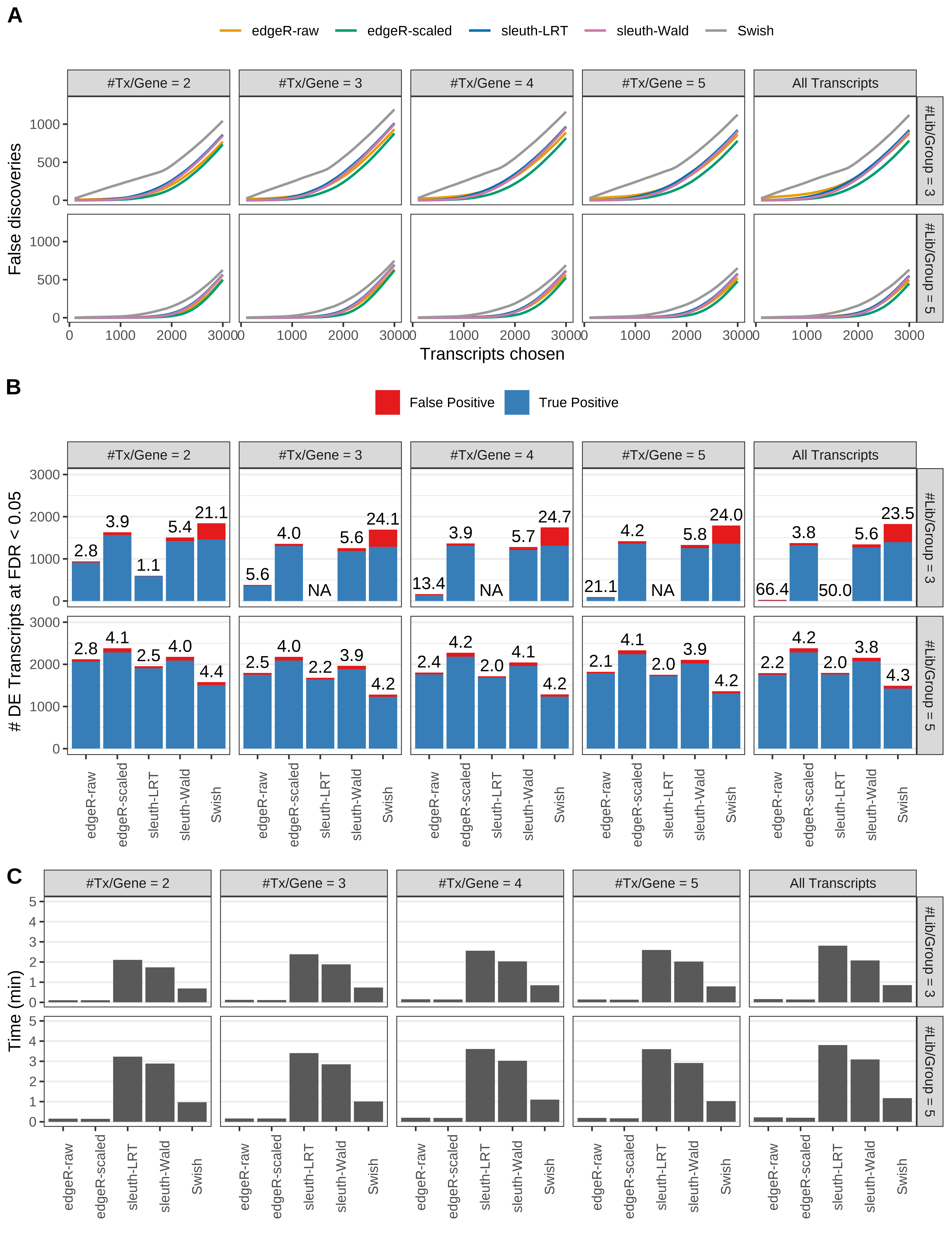
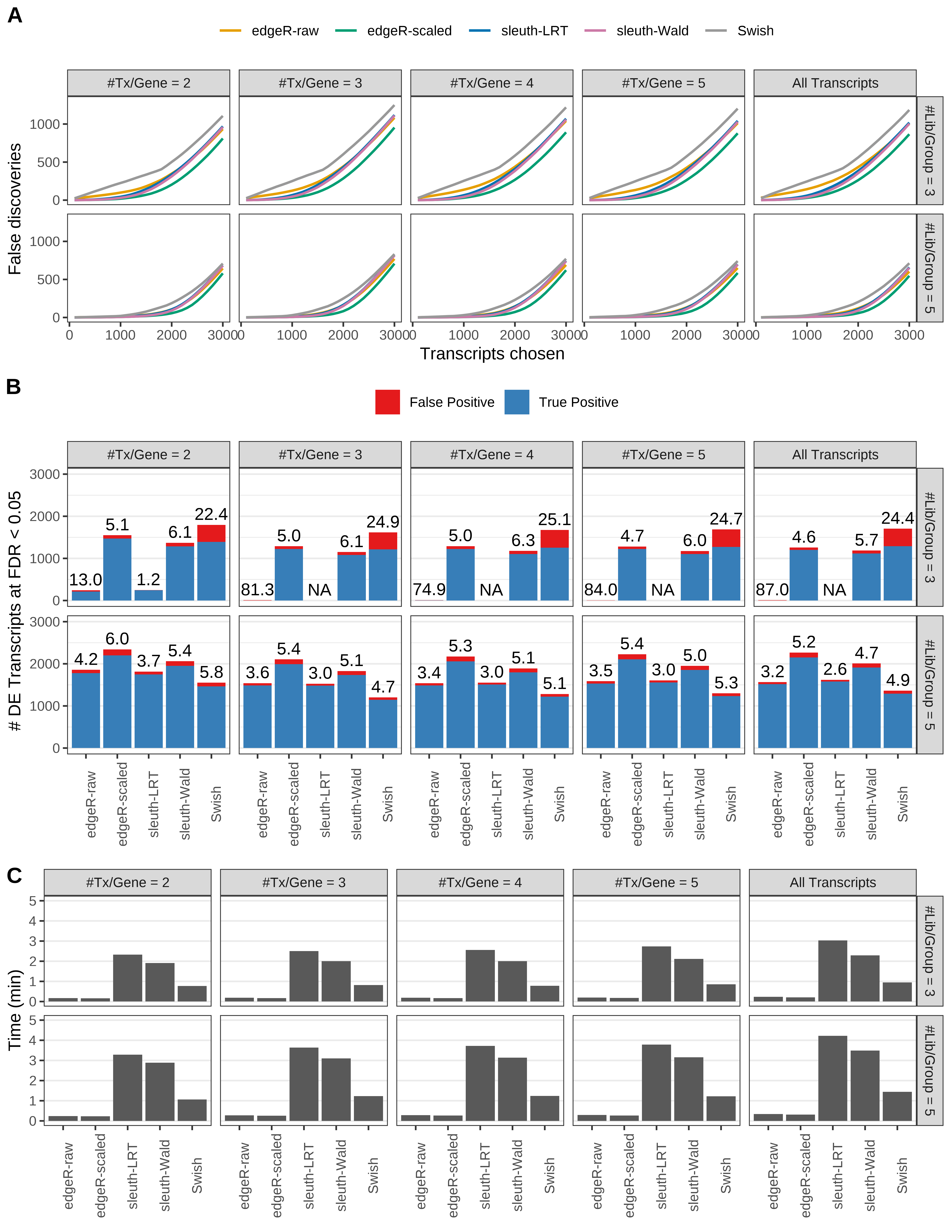
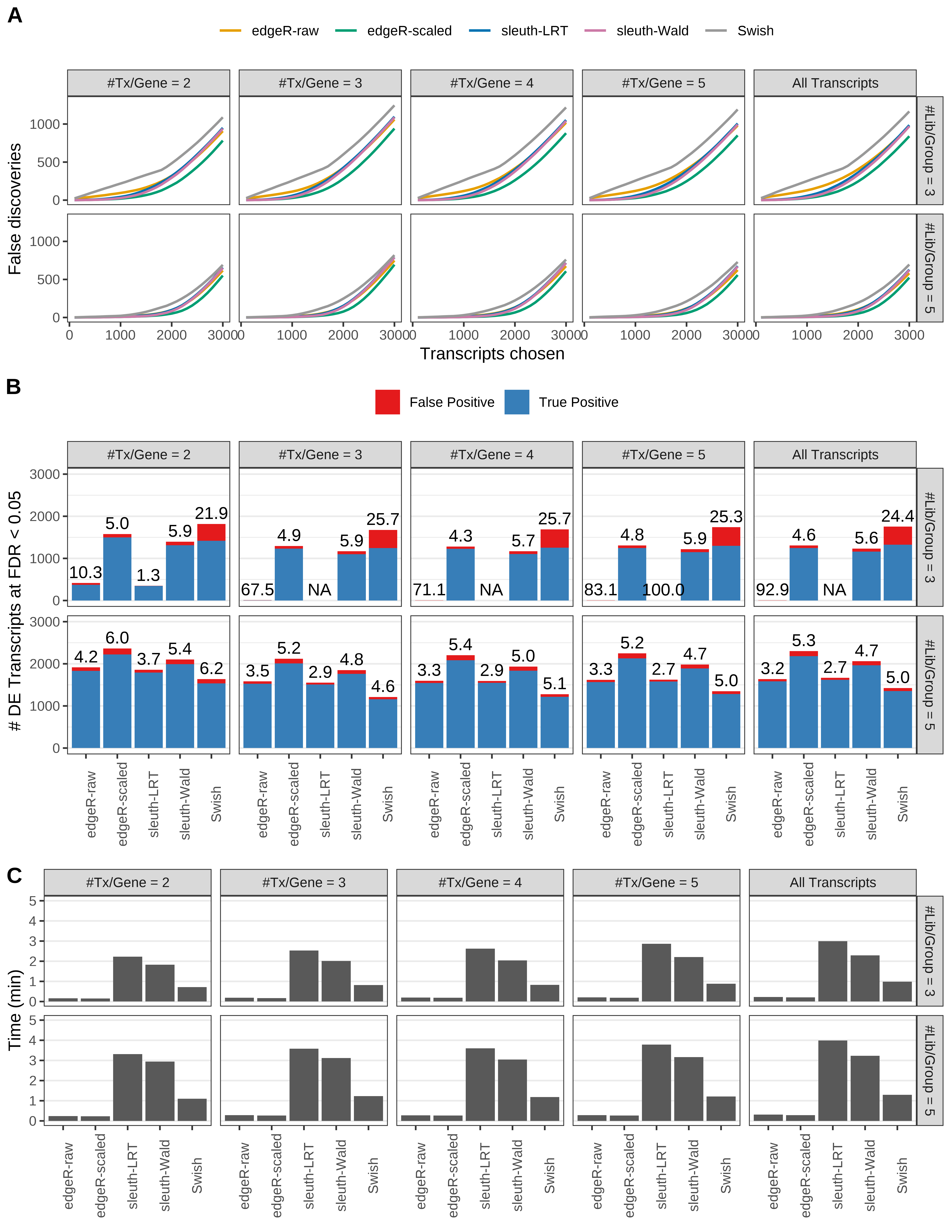
> capA <- paste(cap,
+ '(A) Average number of false discoveries as a function of the number of chosen transcripts.',
+ '(B) Average number of true (blue) and false (red) positive DE transcripts. Observed is FDR annotated.',
+ '(C) Average computing time in minutes.')
>
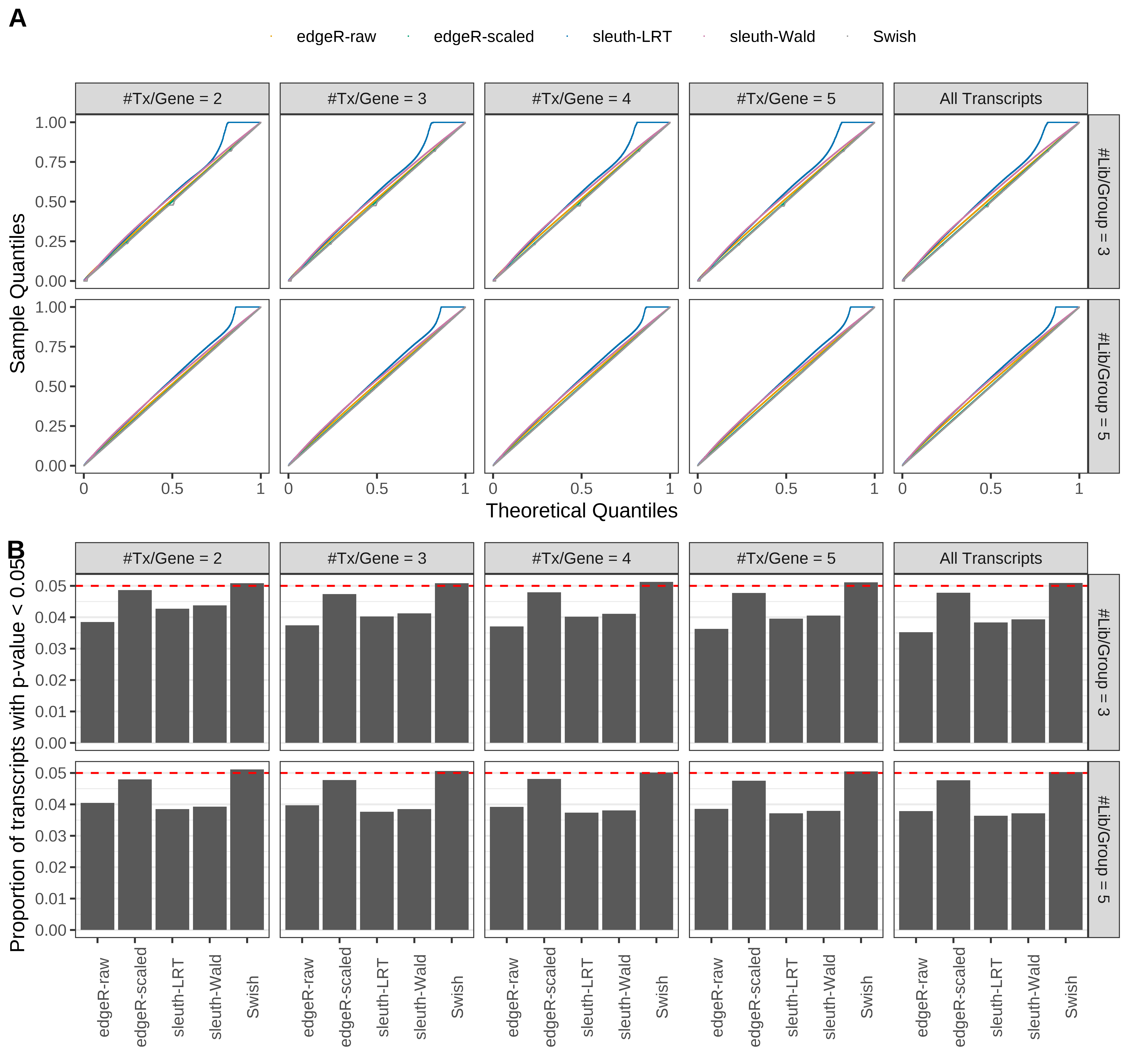
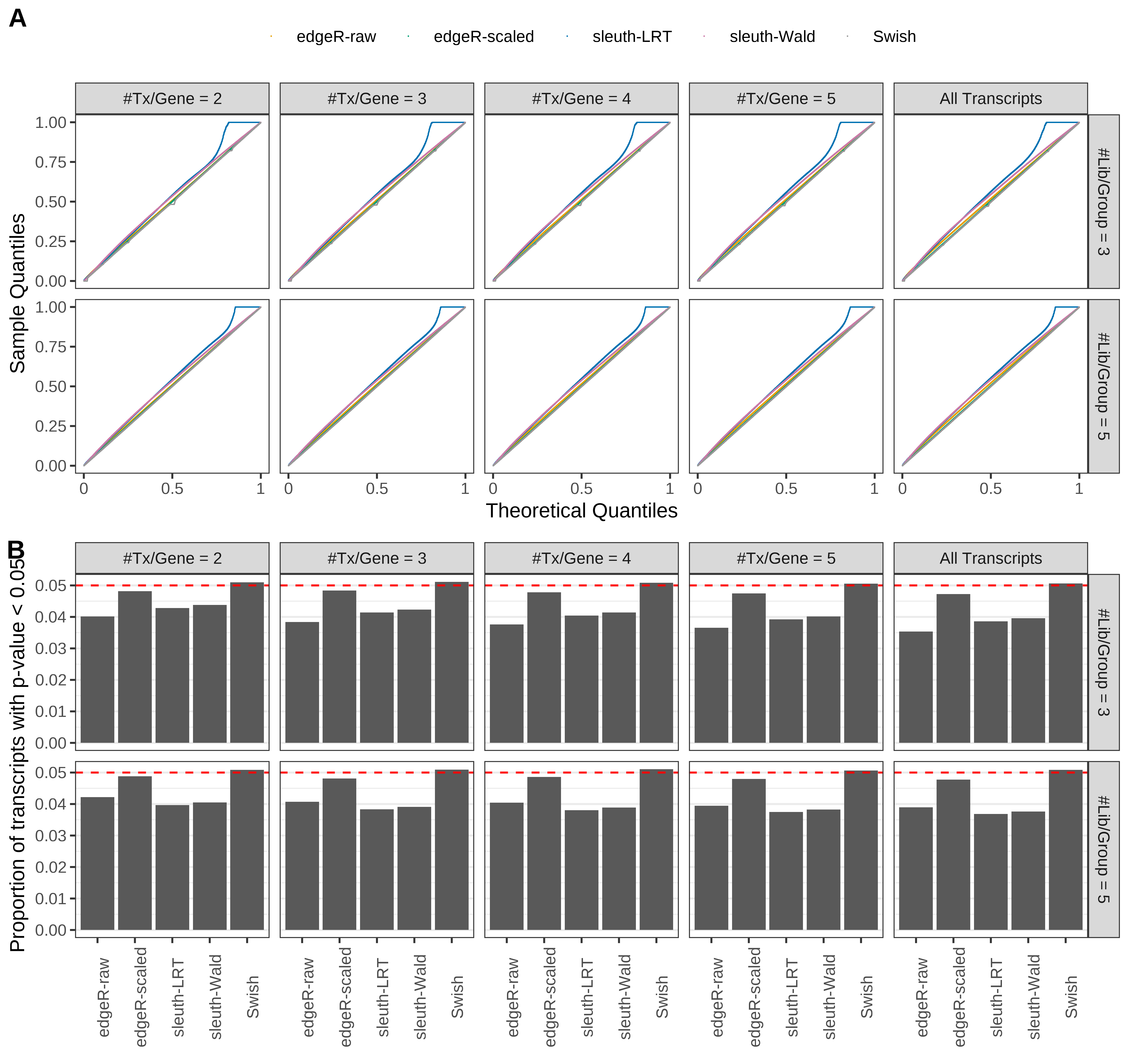
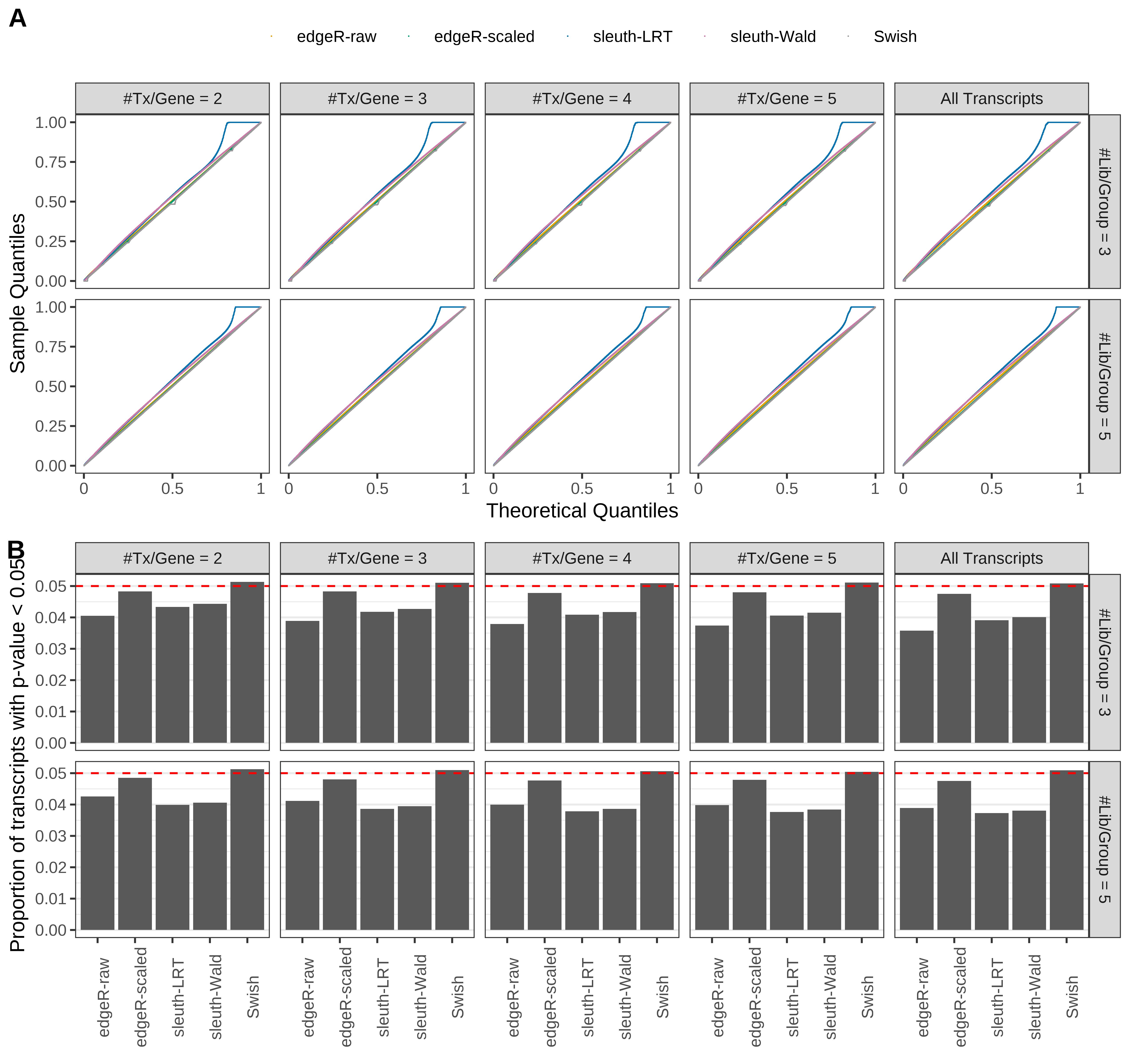
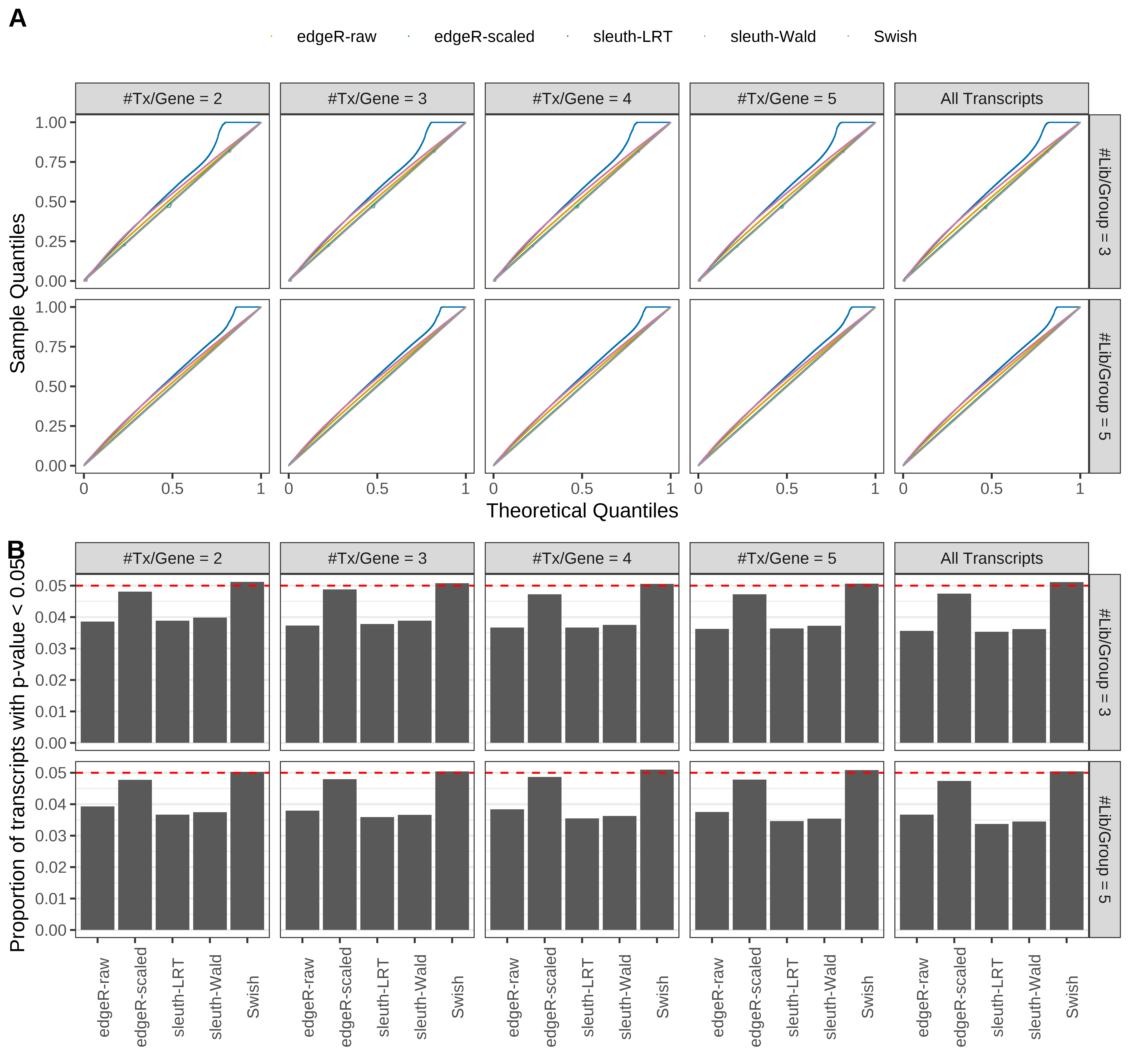
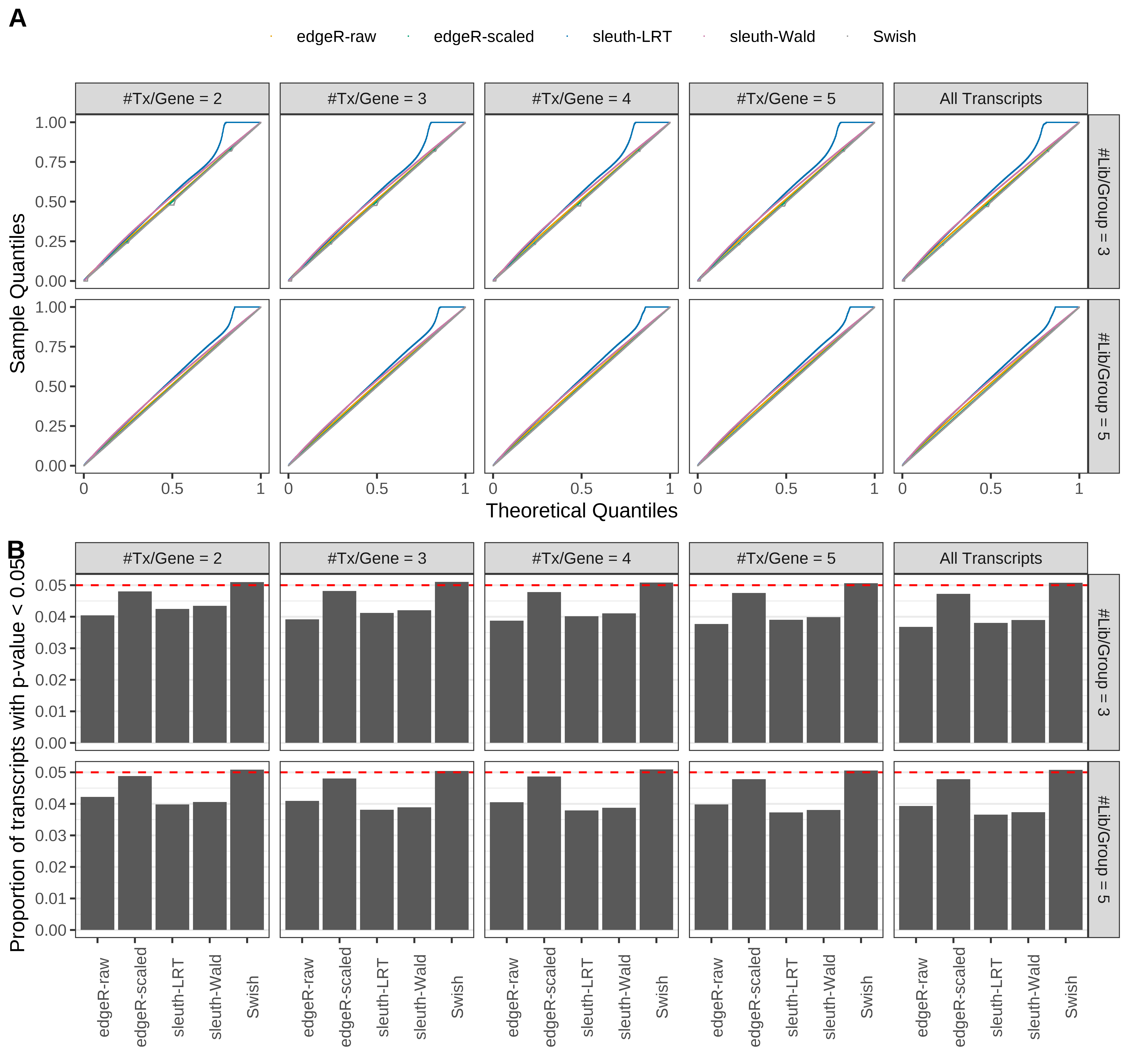
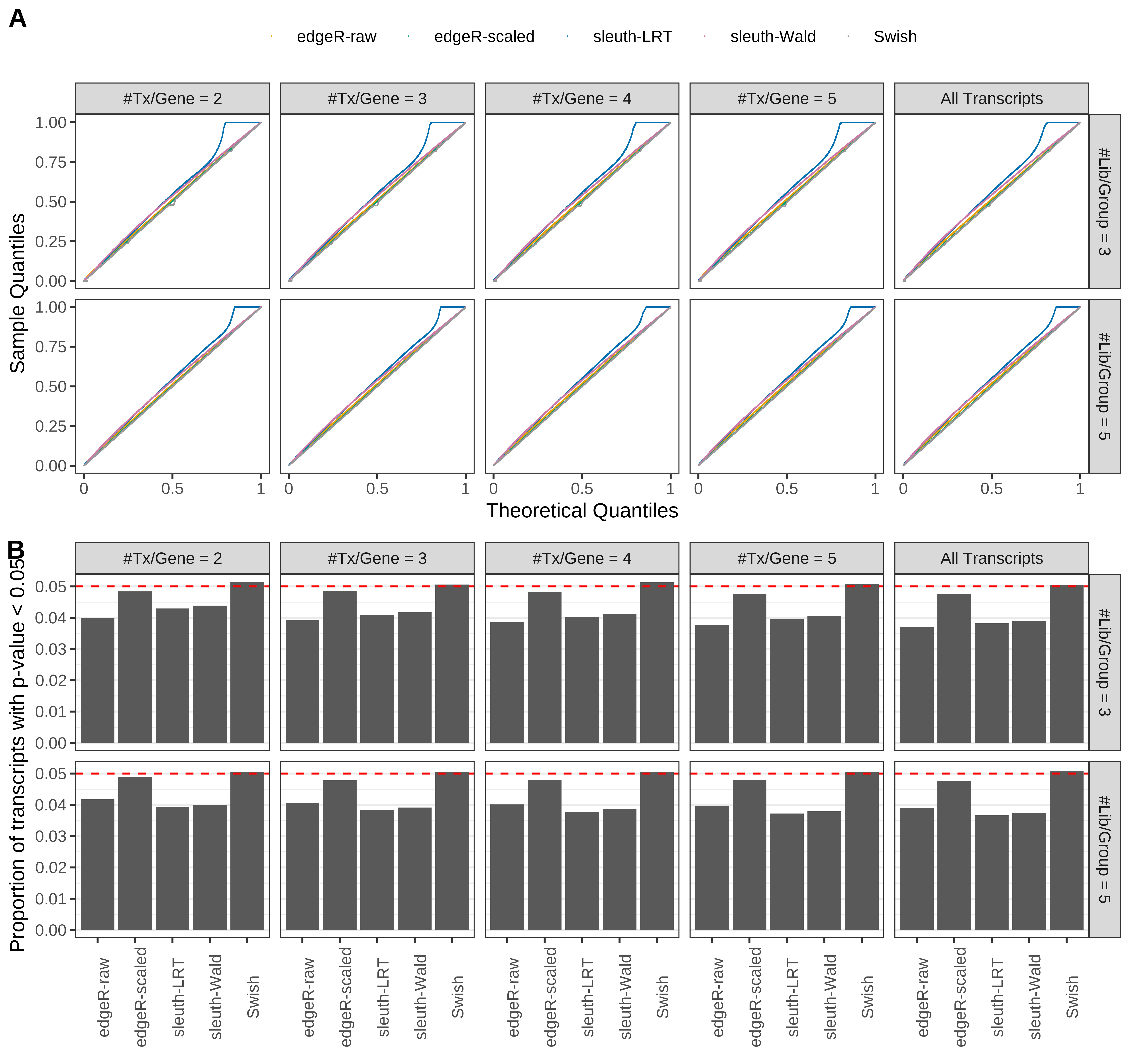
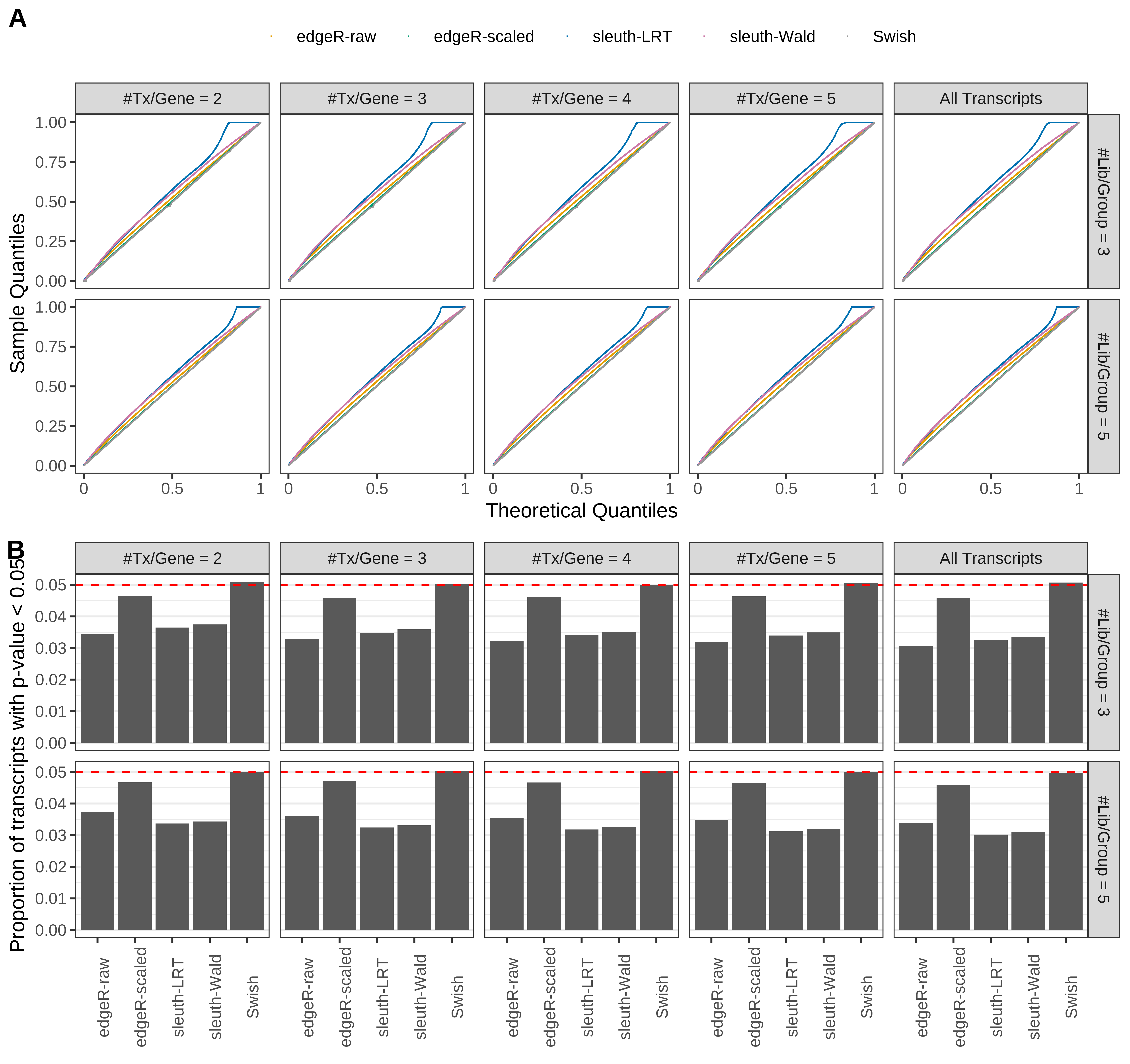
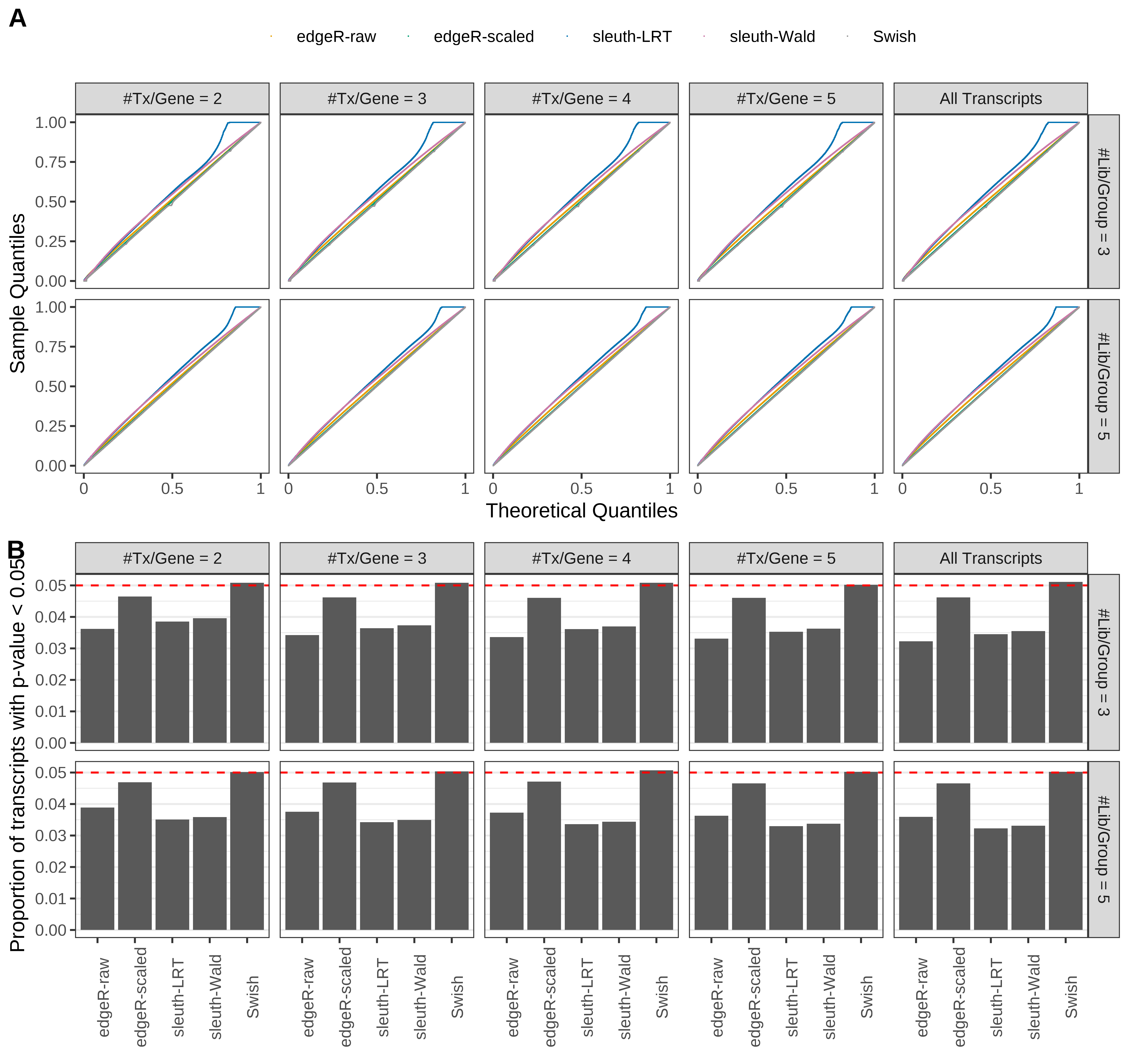
> capB <- paste(cap,
+ '(A) QQ plots of p-values for simulations without any differential expression (averaged over 20 simulations).',
+ '(B) Proportion of transcripts with unadjusted p-values less than 0.05 for simulations without any differential expression (averaged over 20 simulations)')
>
> capC <- paste(cap,
+ '(A) Density histograms for simulations without any differential expression (averaged over 20 simulations).') I also compute the observed power and false discovery rate for different types of reads (paired- or single-end) and read lengths and present them in the same table:
> dt.scenario.table <- expand.grid('genome' = 'mm39',
+                                  'quantifier' = c('Salmon','kallisto'),
+                                  'txpergene' = c(paste0('#Tx/Gene = ',2:5),'All Transcripts'),
+                                  stringsAsFactors = FALSE)
>
> cap.txpergene <- dt.scenario.table$txpergene
> cap.txpergene %<>% mapvalues(from = c(paste0('#Tx/Gene = ',2:5),'All Transcripts'),
+                              to = c(paste0('maximum of ',2:5,' transcripts/gene expressed'),
+                                     'all transcripts expressed'))
>
> cap <- paste0('Simulation results - observed power and false discovery rate for',
+               ' different read types and read Lengths, averaged over 20 simulations. Scenario with ',
+               dt.scenario.table$genome,' genome, ',cap.txpergene,', and reads ',
+               ' quantified with ',dt.scenario.table$quantifier,'.')
>
> cap1 <- paste(cap,'Library size shown in million reads (M) with 25/100 indicating library sizes alternating between 25M and 100M across replicates. Read lengths are shown in base pairs (bp). Red color indicates observed FDR values greater than the nominal 0.05. Blue color indicates most powerful method for a given scenario (row). Empty cells indicate cases in which a method failed to call any transcript as DE.')
We created the table below with the function
tabulateMetrics.
> tables <- lapply(seq_len(nrow(dt.scenario.table)),function(i){
+   scenario <- as.character(dt.scenario.table[i,])
+   names(scenario) <- colnames(dt.scenario.table)
+
+   tb1 <- tabulateMetrics(subsetDT(dt.metrics,scenario = scenario,plot = FALSE),
+                          cap = cap1[i],
+                          format = 'html')
+
+   out <- list('scenario' = scenario,'table1' = tb1)
+
+   return(out)
+ })
Warning in class(mat.fdr) <- "numeric": NAs introduced by coercion

Warning in class(mat.fdr) <- "numeric": NAs introduced by coercion

Warning in class(mat.fdr) <- "numeric": NAs introduced by coercion

Warning in class(mat.fdr) <- "numeric": NAs introduced by coercion

Warning in class(mat.fdr) <- "numeric": NAs introduced by coercion

Warning in class(mat.fdr) <- "numeric": NAs introduced by coercion

Warning in class(mat.fdr) <- "numeric": NAs introduced by coercion

Warning in class(mat.fdr) <- "numeric": NAs introduced by coercion

Warning in class(mat.fdr) <- "numeric": NAs introduced by coercion
> cat('\n\n<!-- -->\n\n')


<!-- -->
Power, false discovery rate, and computing time
Results from power, false discovery rate, and computing time are presented below.
> for(i in seq_len(length(plots))) {
+   fig <- plots[[i]]$panelA
+   print(fig)
+   cat('\n\n<!-- -->\n\n')
+ } 
Simulation results. Scenario with mm39 genome, 50bp single-end reads quantified with Salmon, and balanced libraries. (A) Average number of false discoveries as a function of the number of chosen transcripts. (B) Average number of true (blue) and false (red) positive DE transcripts. Observed is FDR annotated. (C) Average computing time in minutes.
Simulation results. Scenario with mm39 genome, 75bp single-end reads quantified with Salmon, and balanced libraries. (A) Average number of false discoveries as a function of the number of chosen transcripts. (B) Average number of true (blue) and false (red) positive DE transcripts. Observed is FDR annotated. (C) Average computing time in minutes.

Simulation results. Scenario with mm39 genome, 100bp single-end reads quantified with Salmon, and balanced libraries. (A) Average number of false discoveries as a function of the number of chosen transcripts. (B) Average number of true (blue) and false (red) positive DE transcripts. Observed is FDR annotated. (C) Average computing time in minutes.
Simulation results. Scenario with mm39 genome, 125bp single-end reads quantified with Salmon, and balanced libraries. (A) Average number of false discoveries as a function of the number of chosen transcripts. (B) Average number of true (blue) and false (red) positive DE transcripts. Observed is FDR annotated. (C) Average computing time in minutes.
Simulation results. Scenario with mm39 genome, 150bp single-end reads quantified with Salmon, and balanced libraries. (A) Average number of false discoveries as a function of the number of chosen transcripts. (B) Average number of true (blue) and false (red) positive DE transcripts. Observed is FDR annotated. (C) Average computing time in minutes.
Simulation results. Scenario with mm39 genome, 50bp paired-end reads quantified with Salmon, and balanced libraries. (A) Average number of false discoveries as a function of the number of chosen transcripts. (B) Average number of true (blue) and false (red) positive DE transcripts. Observed is FDR annotated. (C) Average computing time in minutes.
Simulation results. Scenario with mm39 genome, 75bp paired-end reads quantified with Salmon, and balanced libraries. (A) Average number of false discoveries as a function of the number of chosen transcripts. (B) Average number of true (blue) and false (red) positive DE transcripts. Observed is FDR annotated. (C) Average computing time in minutes.

Simulation results. Scenario with mm39 genome, 100bp paired-end reads quantified with Salmon, and balanced libraries. (A) Average number of false discoveries as a function of the number of chosen transcripts. (B) Average number of true (blue) and false (red) positive DE transcripts. Observed is FDR annotated. (C) Average computing time in minutes.

Simulation results. Scenario with mm39 genome, 125bp paired-end reads quantified with Salmon, and balanced libraries. (A) Average number of false discoveries as a function of the number of chosen transcripts. (B) Average number of true (blue) and false (red) positive DE transcripts. Observed is FDR annotated. (C) Average computing time in minutes.

Simulation results. Scenario with mm39 genome, 150bp paired-end reads quantified with Salmon, and balanced libraries. (A) Average number of false discoveries as a function of the number of chosen transcripts. (B) Average number of true (blue) and false (red) positive DE transcripts. Observed is FDR annotated. (C) Average computing time in minutes.
Simulation results. Scenario with mm39 genome, 50bp single-end reads quantified with kallisto, and balanced libraries. (A) Average number of false discoveries as a function of the number of chosen transcripts. (B) Average number of true (blue) and false (red) positive DE transcripts. Observed is FDR annotated. (C) Average computing time in minutes.
Simulation results. Scenario with mm39 genome, 75bp single-end reads quantified with kallisto, and balanced libraries. (A) Average number of false discoveries as a function of the number of chosen transcripts. (B) Average number of true (blue) and false (red) positive DE transcripts. Observed is FDR annotated. (C) Average computing time in minutes.
Simulation results. Scenario with mm39 genome, 100bp single-end reads quantified with kallisto, and balanced libraries. (A) Average number of false discoveries as a function of the number of chosen transcripts. (B) Average number of true (blue) and false (red) positive DE transcripts. Observed is FDR annotated. (C) Average computing time in minutes.
Simulation results. Scenario with mm39 genome, 125bp single-end reads quantified with kallisto, and balanced libraries. (A) Average number of false discoveries as a function of the number of chosen transcripts. (B) Average number of true (blue) and false (red) positive DE transcripts. Observed is FDR annotated. (C) Average computing time in minutes.
Simulation results. Scenario with mm39 genome, 150bp single-end reads quantified with kallisto, and balanced libraries. (A) Average number of false discoveries as a function of the number of chosen transcripts. (B) Average number of true (blue) and false (red) positive DE transcripts. Observed is FDR annotated. (C) Average computing time in minutes.

Simulation results. Scenario with mm39 genome, 50bp paired-end reads quantified with kallisto, and balanced libraries. (A) Average number of false discoveries as a function of the number of chosen transcripts. (B) Average number of true (blue) and false (red) positive DE transcripts. Observed is FDR annotated. (C) Average computing time in minutes.

Simulation results. Scenario with mm39 genome, 75bp paired-end reads quantified with kallisto, and balanced libraries. (A) Average number of false discoveries as a function of the number of chosen transcripts. (B) Average number of true (blue) and false (red) positive DE transcripts. Observed is FDR annotated. (C) Average computing time in minutes.

Simulation results. Scenario with mm39 genome, 100bp paired-end reads quantified with kallisto, and balanced libraries. (A) Average number of false discoveries as a function of the number of chosen transcripts. (B) Average number of true (blue) and false (red) positive DE transcripts. Observed is FDR annotated. (C) Average computing time in minutes.

Simulation results. Scenario with mm39 genome, 125bp paired-end reads quantified with kallisto, and balanced libraries. (A) Average number of false discoveries as a function of the number of chosen transcripts. (B) Average number of true (blue) and false (red) positive DE transcripts. Observed is FDR annotated. (C) Average computing time in minutes.

Simulation results. Scenario with mm39 genome, 150bp paired-end reads quantified with kallisto, and balanced libraries. (A) Average number of false discoveries as a function of the number of chosen transcripts. (B) Average number of true (blue) and false (red) positive DE transcripts. Observed is FDR annotated. (C) Average computing time in minutes.

Simulation results. Scenario with mm39 genome, 50bp single-end reads quantified with Salmon, and unbalanced libraries. (A) Average number of false discoveries as a function of the number of chosen transcripts. (B) Average number of true (blue) and false (red) positive DE transcripts. Observed is FDR annotated. (C) Average computing time in minutes.
Simulation results. Scenario with mm39 genome, 75bp single-end reads quantified with Salmon, and unbalanced libraries. (A) Average number of false discoveries as a function of the number of chosen transcripts. (B) Average number of true (blue) and false (red) positive DE transcripts. Observed is FDR annotated. (C) Average computing time in minutes.
Simulation results. Scenario with mm39 genome, 100bp single-end reads quantified with Salmon, and unbalanced libraries. (A) Average number of false discoveries as a function of the number of chosen transcripts. (B) Average number of true (blue) and false (red) positive DE transcripts. Observed is FDR annotated. (C) Average computing time in minutes.

Simulation results. Scenario with mm39 genome, 125bp single-end reads quantified with Salmon, and unbalanced libraries. (A) Average number of false discoveries as a function of the number of chosen transcripts. (B) Average number of true (blue) and false (red) positive DE transcripts. Observed is FDR annotated. (C) Average computing time in minutes.
Simulation results. Scenario with mm39 genome, 150bp single-end reads quantified with Salmon, and unbalanced libraries. (A) Average number of false discoveries as a function of the number of chosen transcripts. (B) Average number of true (blue) and false (red) positive DE transcripts. Observed is FDR annotated. (C) Average computing time in minutes.
Simulation results. Scenario with mm39 genome, 50bp paired-end reads quantified with Salmon, and unbalanced libraries. (A) Average number of false discoveries as a function of the number of chosen transcripts. (B) Average number of true (blue) and false (red) positive DE transcripts. Observed is FDR annotated. (C) Average computing time in minutes.
Simulation results. Scenario with mm39 genome, 75bp paired-end reads quantified with Salmon, and unbalanced libraries. (A) Average number of false discoveries as a function of the number of chosen transcripts. (B) Average number of true (blue) and false (red) positive DE transcripts. Observed is FDR annotated. (C) Average computing time in minutes.
Simulation results. Scenario with mm39 genome, 100bp paired-end reads quantified with Salmon, and unbalanced libraries. (A) Average number of false discoveries as a function of the number of chosen transcripts. (B) Average number of true (blue) and false (red) positive DE transcripts. Observed is FDR annotated. (C) Average computing time in minutes.

Simulation results. Scenario with mm39 genome, 125bp paired-end reads quantified with Salmon, and unbalanced libraries. (A) Average number of false discoveries as a function of the number of chosen transcripts. (B) Average number of true (blue) and false (red) positive DE transcripts. Observed is FDR annotated. (C) Average computing time in minutes.
Simulation results. Scenario with mm39 genome, 150bp paired-end reads quantified with Salmon, and unbalanced libraries. (A) Average number of false discoveries as a function of the number of chosen transcripts. (B) Average number of true (blue) and false (red) positive DE transcripts. Observed is FDR annotated. (C) Average computing time in minutes.

Simulation results. Scenario with mm39 genome, 50bp single-end reads quantified with kallisto, and unbalanced libraries. (A) Average number of false discoveries as a function of the number of chosen transcripts. (B) Average number of true (blue) and false (red) positive DE transcripts. Observed is FDR annotated. (C) Average computing time in minutes.
Simulation results. Scenario with mm39 genome, 75bp single-end reads quantified with kallisto, and unbalanced libraries. (A) Average number of false discoveries as a function of the number of chosen transcripts. (B) Average number of true (blue) and false (red) positive DE transcripts. Observed is FDR annotated. (C) Average computing time in minutes.
Simulation results. Scenario with mm39 genome, 100bp single-end reads quantified with kallisto, and unbalanced libraries. (A) Average number of false discoveries as a function of the number of chosen transcripts. (B) Average number of true (blue) and false (red) positive DE transcripts. Observed is FDR annotated. (C) Average computing time in minutes.
Simulation results. Scenario with mm39 genome, 125bp single-end reads quantified with kallisto, and unbalanced libraries. (A) Average number of false discoveries as a function of the number of chosen transcripts. (B) Average number of true (blue) and false (red) positive DE transcripts. Observed is FDR annotated. (C) Average computing time in minutes.
Simulation results. Scenario with mm39 genome, 150bp single-end reads quantified with kallisto, and unbalanced libraries. (A) Average number of false discoveries as a function of the number of chosen transcripts. (B) Average number of true (blue) and false (red) positive DE transcripts. Observed is FDR annotated. (C) Average computing time in minutes.
Simulation results. Scenario with mm39 genome, 50bp paired-end reads quantified with kallisto, and unbalanced libraries. (A) Average number of false discoveries as a function of the number of chosen transcripts. (B) Average number of true (blue) and false (red) positive DE transcripts. Observed is FDR annotated. (C) Average computing time in minutes.
Simulation results. Scenario with mm39 genome, 75bp paired-end reads quantified with kallisto, and unbalanced libraries. (A) Average number of false discoveries as a function of the number of chosen transcripts. (B) Average number of true (blue) and false (red) positive DE transcripts. Observed is FDR annotated. (C) Average computing time in minutes.

Simulation results. Scenario with mm39 genome, 100bp paired-end reads quantified with kallisto, and unbalanced libraries. (A) Average number of false discoveries as a function of the number of chosen transcripts. (B) Average number of true (blue) and false (red) positive DE transcripts. Observed is FDR annotated. (C) Average computing time in minutes.
Simulation results. Scenario with mm39 genome, 125bp paired-end reads quantified with kallisto, and unbalanced libraries. (A) Average number of false discoveries as a function of the number of chosen transcripts. (B) Average number of true (blue) and false (red) positive DE transcripts. Observed is FDR annotated. (C) Average computing time in minutes.

Simulation results. Scenario with mm39 genome, 150bp paired-end reads quantified with kallisto, and unbalanced libraries. (A) Average number of false discoveries as a function of the number of chosen transcripts. (B) Average number of true (blue) and false (red) positive DE transcripts. Observed is FDR annotated. (C) Average computing time in minutes.
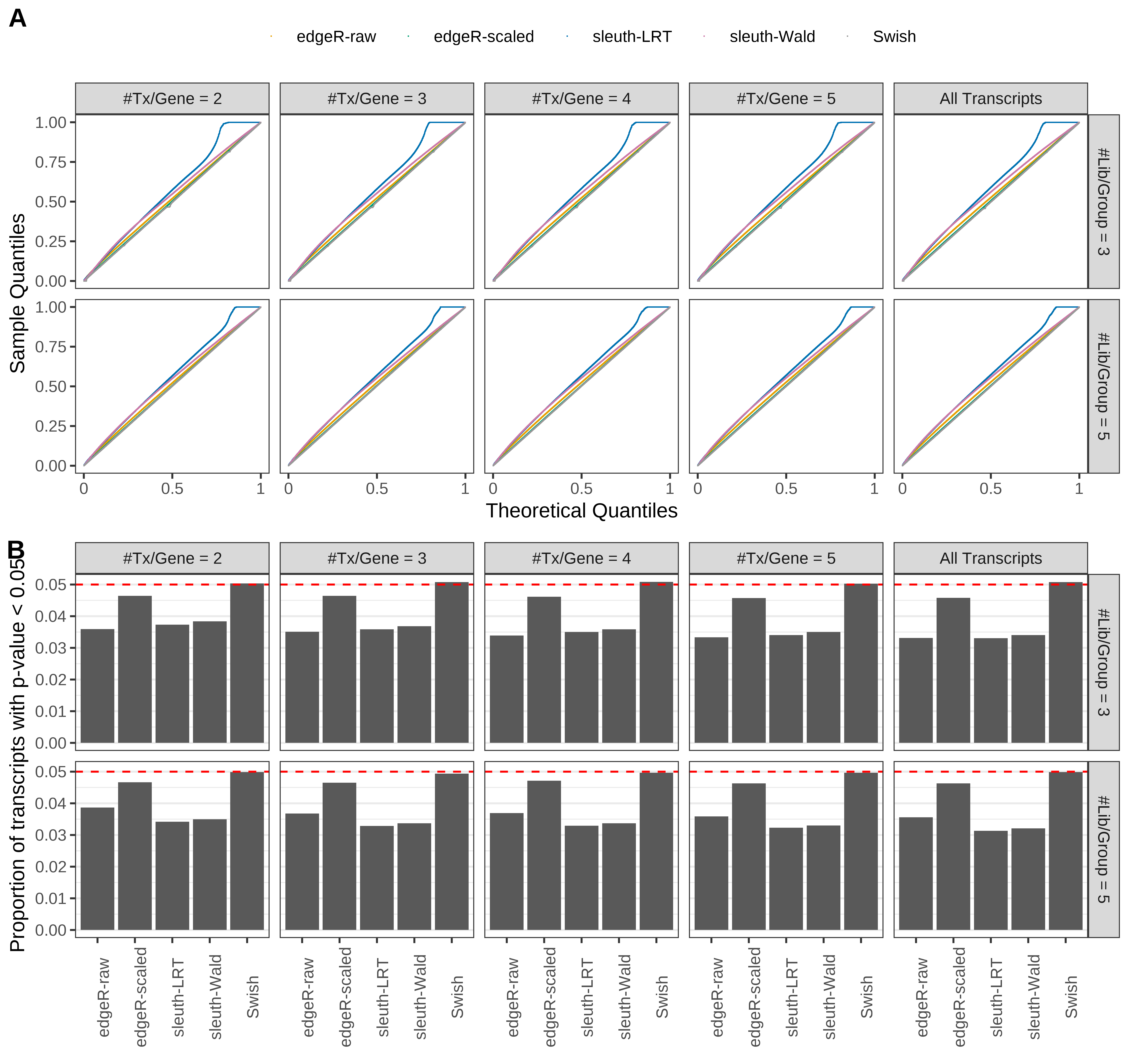
Type 1 error rate control
From null simulations, we present below the results for the type 1 error rate assessment.
> for(i in seq_len(length(plots))) {
+   fig <- plots[[i]]$panelB
+   print(fig)
+   cat('\n\n<!-- -->\n\n')
+ } 
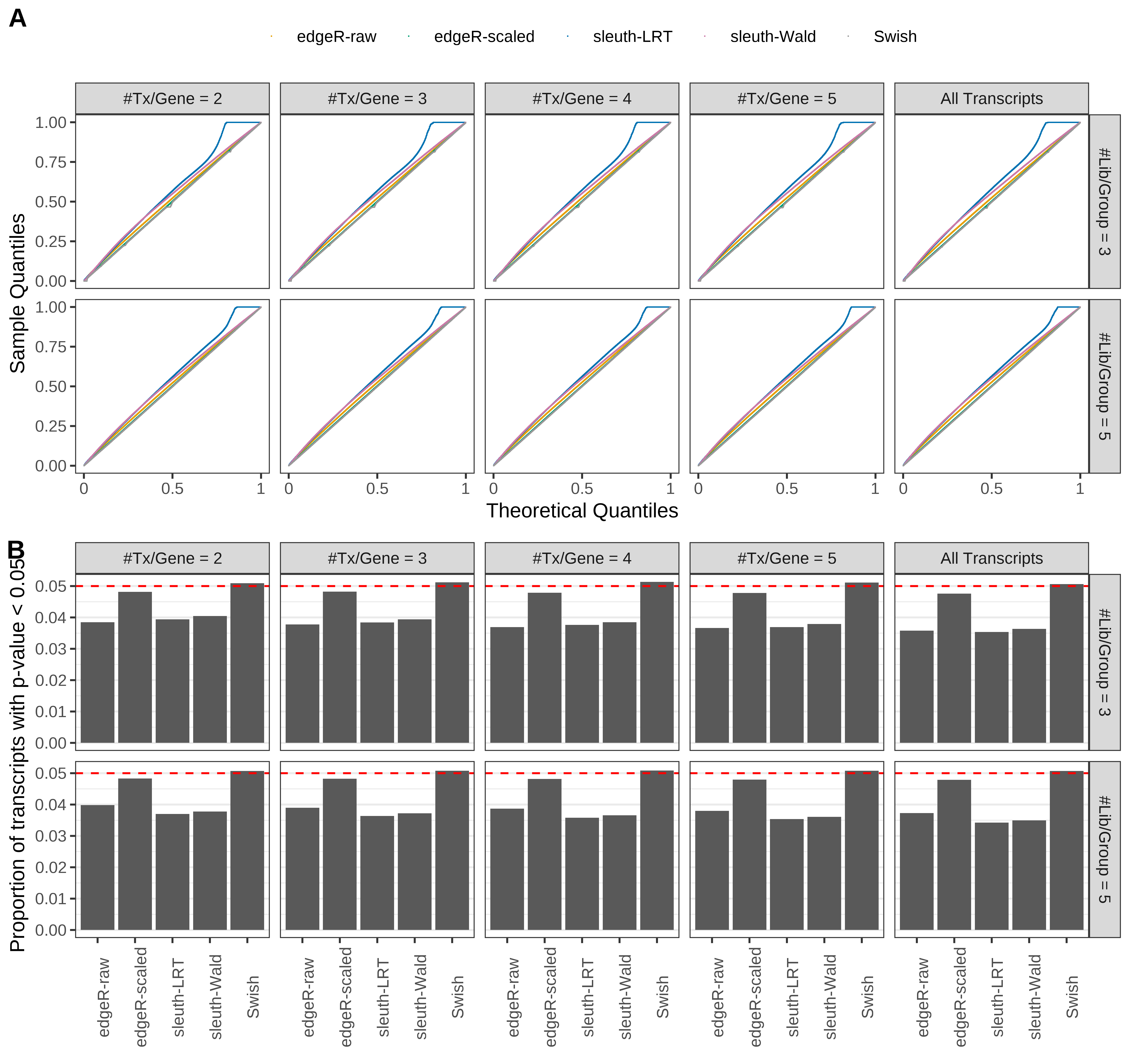
Simulation results. Scenario with mm39 genome, 50bp single-end reads quantified with Salmon, and balanced libraries. (A) QQ plots of p-values for simulations without any differential expression (averaged over 20 simulations). (B) Proportion of transcripts with unadjusted p-values less than 0.05 for simulations without any differential expression (averaged over 20 simulations)
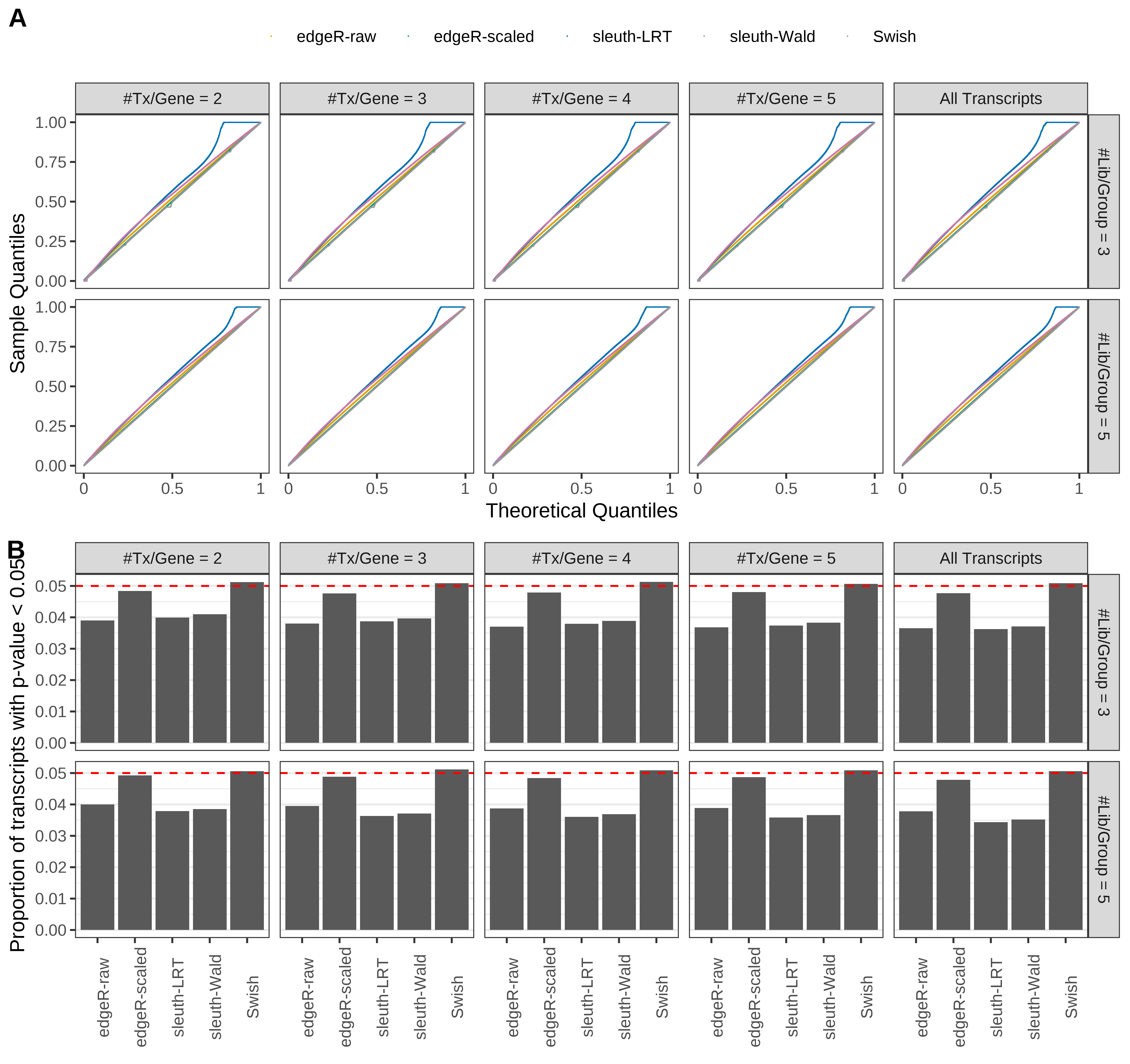
Simulation results. Scenario with mm39 genome, 75bp single-end reads quantified with Salmon, and balanced libraries. (A) QQ plots of p-values for simulations without any differential expression (averaged over 20 simulations). (B) Proportion of transcripts with unadjusted p-values less than 0.05 for simulations without any differential expression (averaged over 20 simulations)
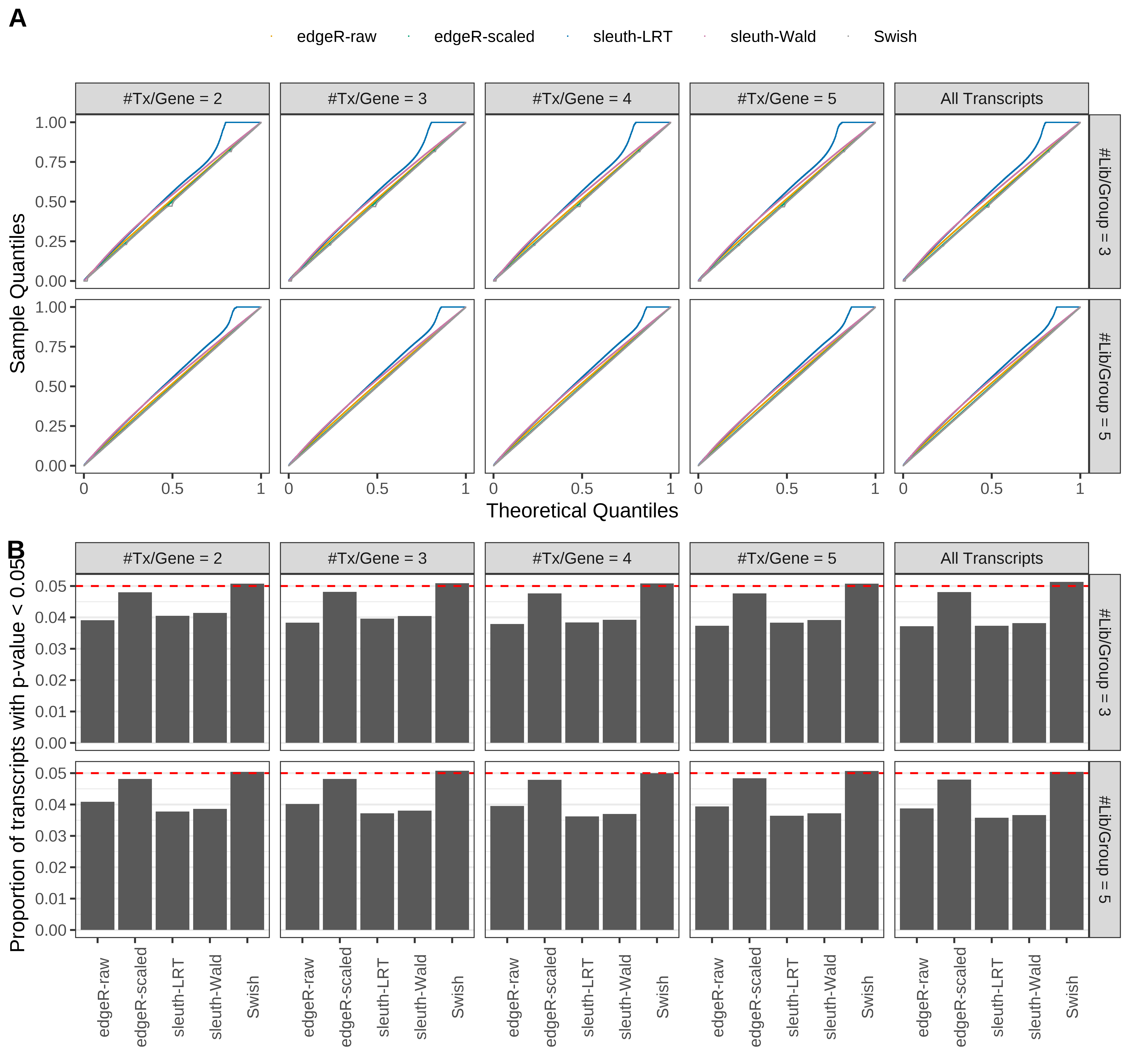
Simulation results. Scenario with mm39 genome, 100bp single-end reads quantified with Salmon, and balanced libraries. (A) QQ plots of p-values for simulations without any differential expression (averaged over 20 simulations). (B) Proportion of transcripts with unadjusted p-values less than 0.05 for simulations without any differential expression (averaged over 20 simulations)

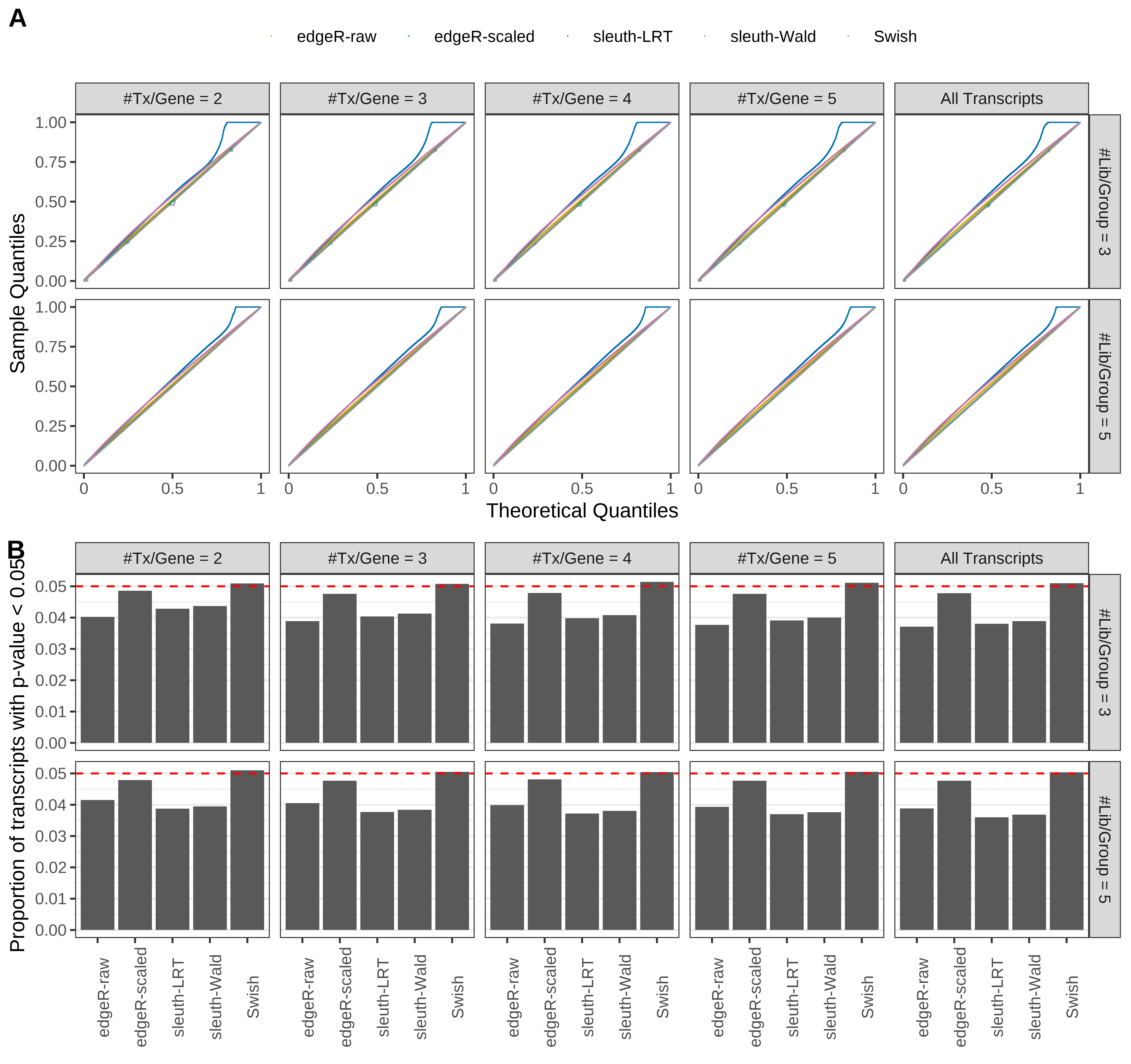
Simulation results. Scenario with mm39 genome, 125bp single-end reads quantified with Salmon, and balanced libraries. (A) QQ plots of p-values for simulations without any differential expression (averaged over 20 simulations). (B) Proportion of transcripts with unadjusted p-values less than 0.05 for simulations without any differential expression (averaged over 20 simulations)

Simulation results. Scenario with mm39 genome, 150bp single-end reads quantified with Salmon, and balanced libraries. (A) QQ plots of p-values for simulations without any differential expression (averaged over 20 simulations). (B) Proportion of transcripts with unadjusted p-values less than 0.05 for simulations without any differential expression (averaged over 20 simulations)
Simulation results. Scenario with mm39 genome, 50bp paired-end reads quantified with Salmon, and balanced libraries. (A) QQ plots of p-values for simulations without any differential expression (averaged over 20 simulations). (B) Proportion of transcripts with unadjusted p-values less than 0.05 for simulations without any differential expression (averaged over 20 simulations)
Simulation results. Scenario with mm39 genome, 75bp paired-end reads quantified with Salmon, and balanced libraries. (A) QQ plots of p-values for simulations without any differential expression (averaged over 20 simulations). (B) Proportion of transcripts with unadjusted p-values less than 0.05 for simulations without any differential expression (averaged over 20 simulations)

Simulation results. Scenario with mm39 genome, 100bp paired-end reads quantified with Salmon, and balanced libraries. (A) QQ plots of p-values for simulations without any differential expression (averaged over 20 simulations). (B) Proportion of transcripts with unadjusted p-values less than 0.05 for simulations without any differential expression (averaged over 20 simulations)
Simulation results. Scenario with mm39 genome, 125bp paired-end reads quantified with Salmon, and balanced libraries. (A) QQ plots of p-values for simulations without any differential expression (averaged over 20 simulations). (B) Proportion of transcripts with unadjusted p-values less than 0.05 for simulations without any differential expression (averaged over 20 simulations)

Simulation results. Scenario with mm39 genome, 150bp paired-end reads quantified with Salmon, and balanced libraries. (A) QQ plots of p-values for simulations without any differential expression (averaged over 20 simulations). (B) Proportion of transcripts with unadjusted p-values less than 0.05 for simulations without any differential expression (averaged over 20 simulations)
Simulation results. Scenario with mm39 genome, 50bp single-end reads quantified with kallisto, and balanced libraries. (A) QQ plots of p-values for simulations without any differential expression (averaged over 20 simulations). (B) Proportion of transcripts with unadjusted p-values less than 0.05 for simulations without any differential expression (averaged over 20 simulations)
Simulation results. Scenario with mm39 genome, 75bp single-end reads quantified with kallisto, and balanced libraries. (A) QQ plots of p-values for simulations without any differential expression (averaged over 20 simulations). (B) Proportion of transcripts with unadjusted p-values less than 0.05 for simulations without any differential expression (averaged over 20 simulations)
Simulation results. Scenario with mm39 genome, 100bp single-end reads quantified with kallisto, and balanced libraries. (A) QQ plots of p-values for simulations without any differential expression (averaged over 20 simulations). (B) Proportion of transcripts with unadjusted p-values less than 0.05 for simulations without any differential expression (averaged over 20 simulations)

Simulation results. Scenario with mm39 genome, 125bp single-end reads quantified with kallisto, and balanced libraries. (A) QQ plots of p-values for simulations without any differential expression (averaged over 20 simulations). (B) Proportion of transcripts with unadjusted p-values less than 0.05 for simulations without any differential expression (averaged over 20 simulations)
Simulation results. Scenario with mm39 genome, 150bp single-end reads quantified with kallisto, and balanced libraries. (A) QQ plots of p-values for simulations without any differential expression (averaged over 20 simulations). (B) Proportion of transcripts with unadjusted p-values less than 0.05 for simulations without any differential expression (averaged over 20 simulations)
Simulation results. Scenario with mm39 genome, 50bp paired-end reads quantified with kallisto, and balanced libraries. (A) QQ plots of p-values for simulations without any differential expression (averaged over 20 simulations). (B) Proportion of transcripts with unadjusted p-values less than 0.05 for simulations without any differential expression (averaged over 20 simulations)
Simulation results. Scenario with mm39 genome, 75bp paired-end reads quantified with kallisto, and balanced libraries. (A) QQ plots of p-values for simulations without any differential expression (averaged over 20 simulations). (B) Proportion of transcripts with unadjusted p-values less than 0.05 for simulations without any differential expression (averaged over 20 simulations)
Simulation results. Scenario with mm39 genome, 100bp paired-end reads quantified with kallisto, and balanced libraries. (A) QQ plots of p-values for simulations without any differential expression (averaged over 20 simulations). (B) Proportion of transcripts with unadjusted p-values less than 0.05 for simulations without any differential expression (averaged over 20 simulations)

Simulation results. Scenario with mm39 genome, 125bp paired-end reads quantified with kallisto, and balanced libraries. (A) QQ plots of p-values for simulations without any differential expression (averaged over 20 simulations). (B) Proportion of transcripts with unadjusted p-values less than 0.05 for simulations without any differential expression (averaged over 20 simulations)

Simulation results. Scenario with mm39 genome, 150bp paired-end reads quantified with kallisto, and balanced libraries. (A) QQ plots of p-values for simulations without any differential expression (averaged over 20 simulations). (B) Proportion of transcripts with unadjusted p-values less than 0.05 for simulations without any differential expression (averaged over 20 simulations)
Simulation results. Scenario with mm39 genome, 50bp single-end reads quantified with Salmon, and unbalanced libraries. (A) QQ plots of p-values for simulations without any differential expression (averaged over 20 simulations). (B) Proportion of transcripts with unadjusted p-values less than 0.05 for simulations without any differential expression (averaged over 20 simulations)

Simulation results. Scenario with mm39 genome, 75bp single-end reads quantified with Salmon, and unbalanced libraries. (A) QQ plots of p-values for simulations without any differential expression (averaged over 20 simulations). (B) Proportion of transcripts with unadjusted p-values less than 0.05 for simulations without any differential expression (averaged over 20 simulations)

Simulation results. Scenario with mm39 genome, 100bp single-end reads quantified with Salmon, and unbalanced libraries. (A) QQ plots of p-values for simulations without any differential expression (averaged over 20 simulations). (B) Proportion of transcripts with unadjusted p-values less than 0.05 for simulations without any differential expression (averaged over 20 simulations)
Simulation results. Scenario with mm39 genome, 125bp single-end reads quantified with Salmon, and unbalanced libraries. (A) QQ plots of p-values for simulations without any differential expression (averaged over 20 simulations). (B) Proportion of transcripts with unadjusted p-values less than 0.05 for simulations without any differential expression (averaged over 20 simulations)
Simulation results. Scenario with mm39 genome, 150bp single-end reads quantified with Salmon, and unbalanced libraries. (A) QQ plots of p-values for simulations without any differential expression (averaged over 20 simulations). (B) Proportion of transcripts with unadjusted p-values less than 0.05 for simulations without any differential expression (averaged over 20 simulations)

Simulation results. Scenario with mm39 genome, 50bp paired-end reads quantified with Salmon, and unbalanced libraries. (A) QQ plots of p-values for simulations without any differential expression (averaged over 20 simulations). (B) Proportion of transcripts with unadjusted p-values less than 0.05 for simulations without any differential expression (averaged over 20 simulations)

Simulation results. Scenario with mm39 genome, 75bp paired-end reads quantified with Salmon, and unbalanced libraries. (A) QQ plots of p-values for simulations without any differential expression (averaged over 20 simulations). (B) Proportion of transcripts with unadjusted p-values less than 0.05 for simulations without any differential expression (averaged over 20 simulations)

Simulation results. Scenario with mm39 genome, 100bp paired-end reads quantified with Salmon, and unbalanced libraries. (A) QQ plots of p-values for simulations without any differential expression (averaged over 20 simulations). (B) Proportion of transcripts with unadjusted p-values less than 0.05 for simulations without any differential expression (averaged over 20 simulations)
Simulation results. Scenario with mm39 genome, 125bp paired-end reads quantified with Salmon, and unbalanced libraries. (A) QQ plots of p-values for simulations without any differential expression (averaged over 20 simulations). (B) Proportion of transcripts with unadjusted p-values less than 0.05 for simulations without any differential expression (averaged over 20 simulations)

Simulation results. Scenario with mm39 genome, 150bp paired-end reads quantified with Salmon, and unbalanced libraries. (A) QQ plots of p-values for simulations without any differential expression (averaged over 20 simulations). (B) Proportion of transcripts with unadjusted p-values less than 0.05 for simulations without any differential expression (averaged over 20 simulations)
Simulation results. Scenario with mm39 genome, 50bp single-end reads quantified with kallisto, and unbalanced libraries. (A) QQ plots of p-values for simulations without any differential expression (averaged over 20 simulations). (B) Proportion of transcripts with unadjusted p-values less than 0.05 for simulations without any differential expression (averaged over 20 simulations)
Simulation results. Scenario with mm39 genome, 75bp single-end reads quantified with kallisto, and unbalanced libraries. (A) QQ plots of p-values for simulations without any differential expression (averaged over 20 simulations). (B) Proportion of transcripts with unadjusted p-values less than 0.05 for simulations without any differential expression (averaged over 20 simulations)
Simulation results. Scenario with mm39 genome, 100bp single-end reads quantified with kallisto, and unbalanced libraries. (A) QQ plots of p-values for simulations without any differential expression (averaged over 20 simulations). (B) Proportion of transcripts with unadjusted p-values less than 0.05 for simulations without any differential expression (averaged over 20 simulations)
Simulation results. Scenario with mm39 genome, 125bp single-end reads quantified with kallisto, and unbalanced libraries. (A) QQ plots of p-values for simulations without any differential expression (averaged over 20 simulations). (B) Proportion of transcripts with unadjusted p-values less than 0.05 for simulations without any differential expression (averaged over 20 simulations)
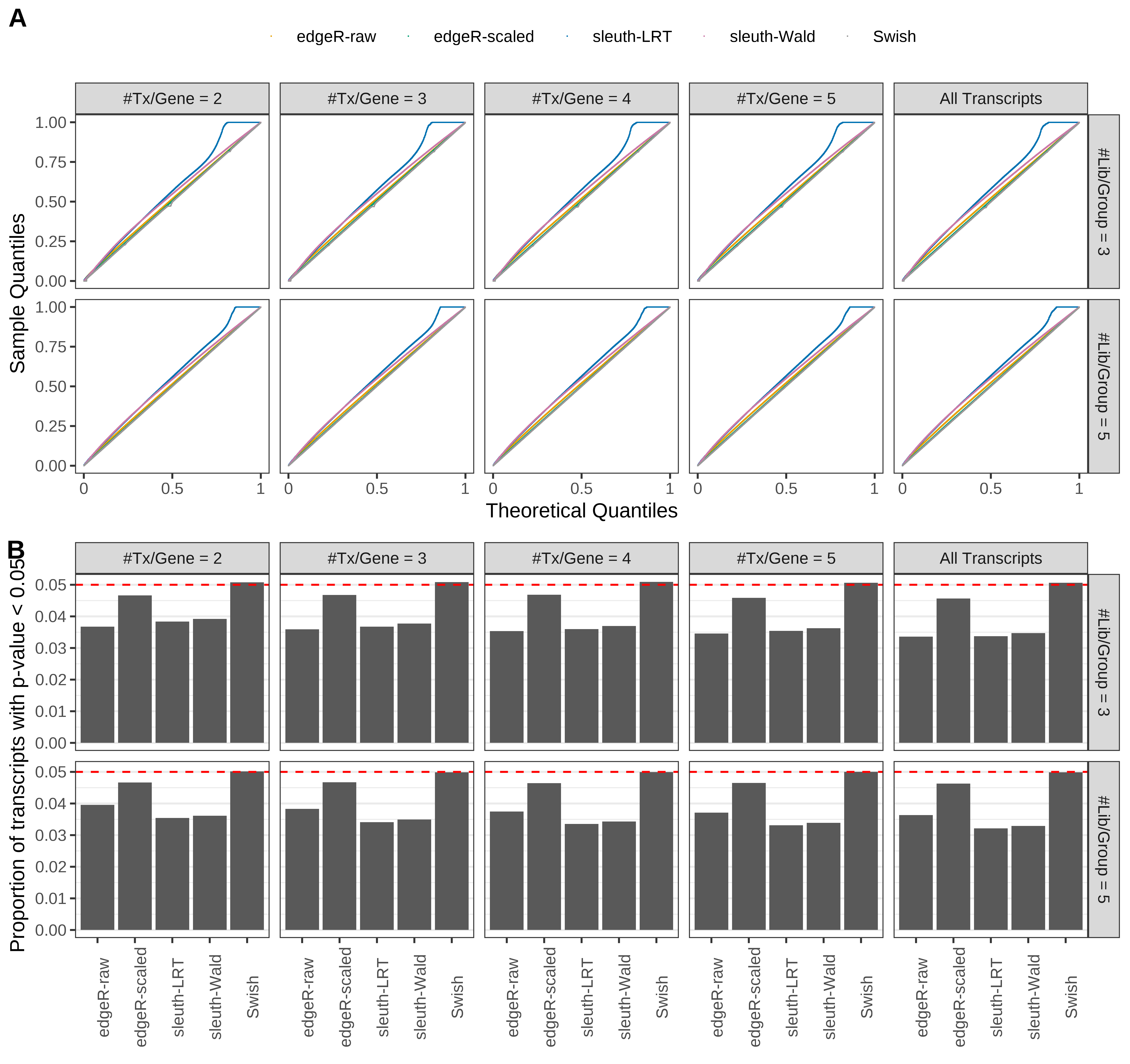
Simulation results. Scenario with mm39 genome, 150bp single-end reads quantified with kallisto, and unbalanced libraries. (A) QQ plots of p-values for simulations without any differential expression (averaged over 20 simulations). (B) Proportion of transcripts with unadjusted p-values less than 0.05 for simulations without any differential expression (averaged over 20 simulations)
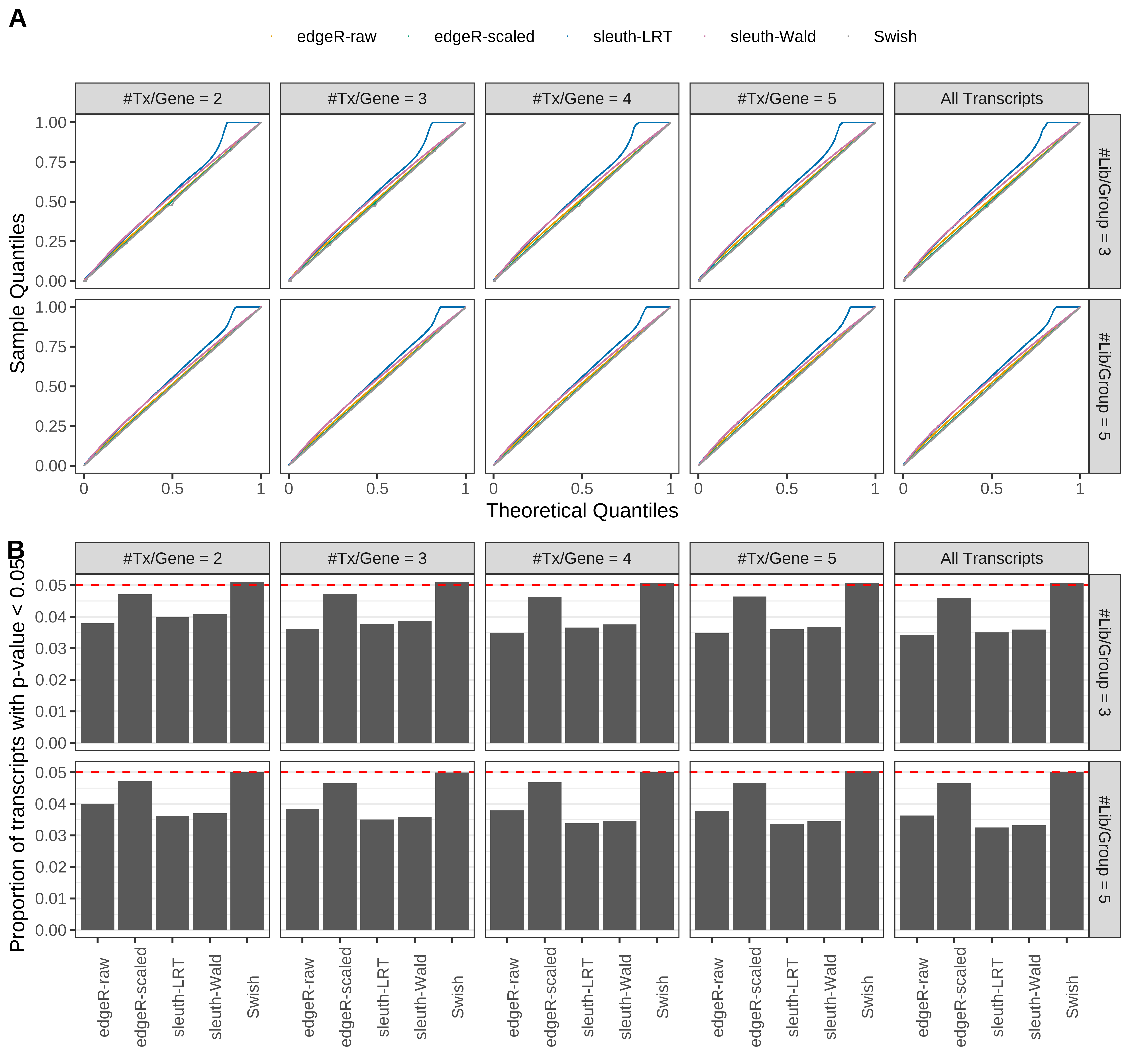
Simulation results. Scenario with mm39 genome, 50bp paired-end reads quantified with kallisto, and unbalanced libraries. (A) QQ plots of p-values for simulations without any differential expression (averaged over 20 simulations). (B) Proportion of transcripts with unadjusted p-values less than 0.05 for simulations without any differential expression (averaged over 20 simulations)
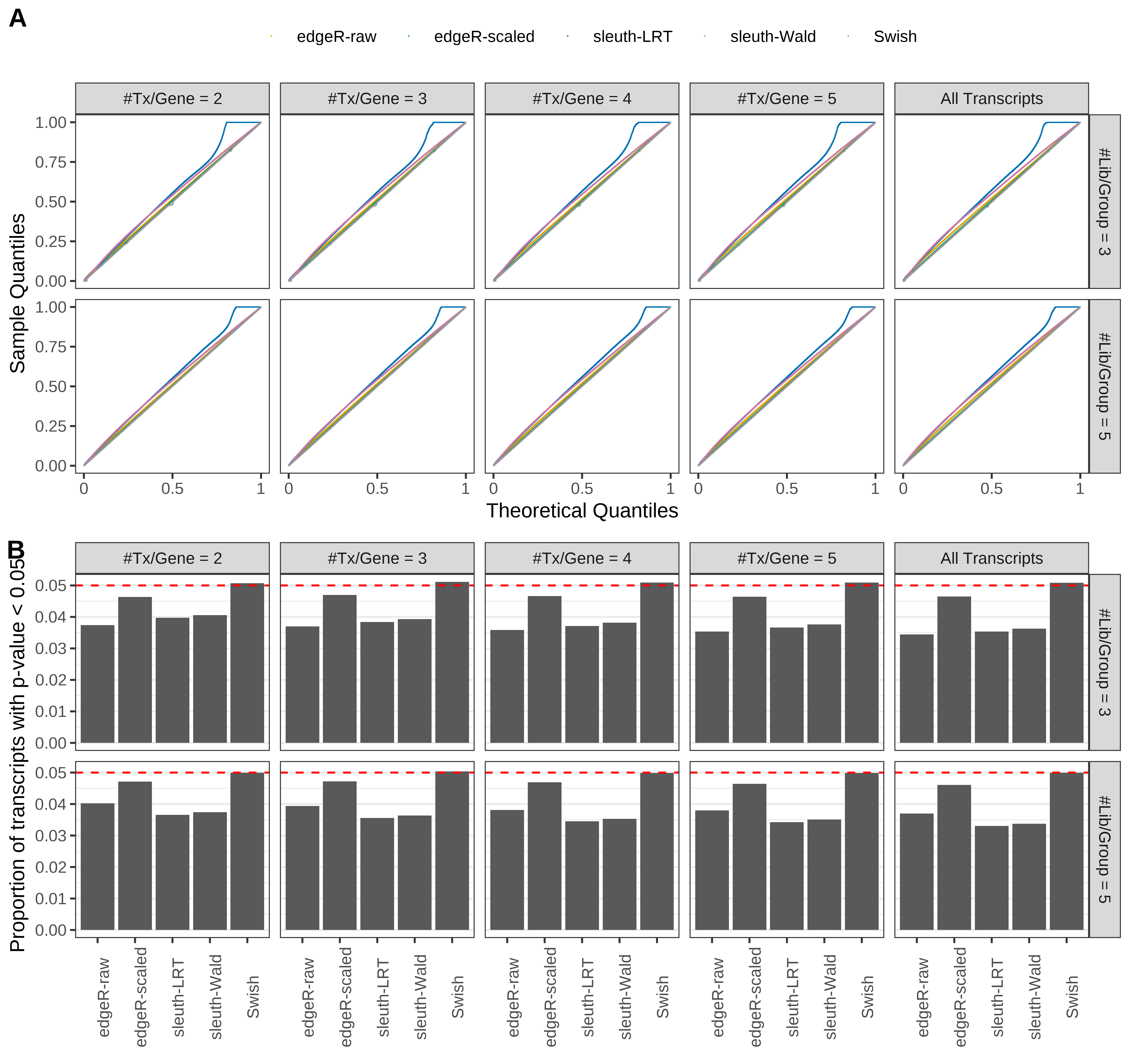
Simulation results. Scenario with mm39 genome, 75bp paired-end reads quantified with kallisto, and unbalanced libraries. (A) QQ plots of p-values for simulations without any differential expression (averaged over 20 simulations). (B) Proportion of transcripts with unadjusted p-values less than 0.05 for simulations without any differential expression (averaged over 20 simulations)

Simulation results. Scenario with mm39 genome, 100bp paired-end reads quantified with kallisto, and unbalanced libraries. (A) QQ plots of p-values for simulations without any differential expression (averaged over 20 simulations). (B) Proportion of transcripts with unadjusted p-values less than 0.05 for simulations without any differential expression (averaged over 20 simulations)
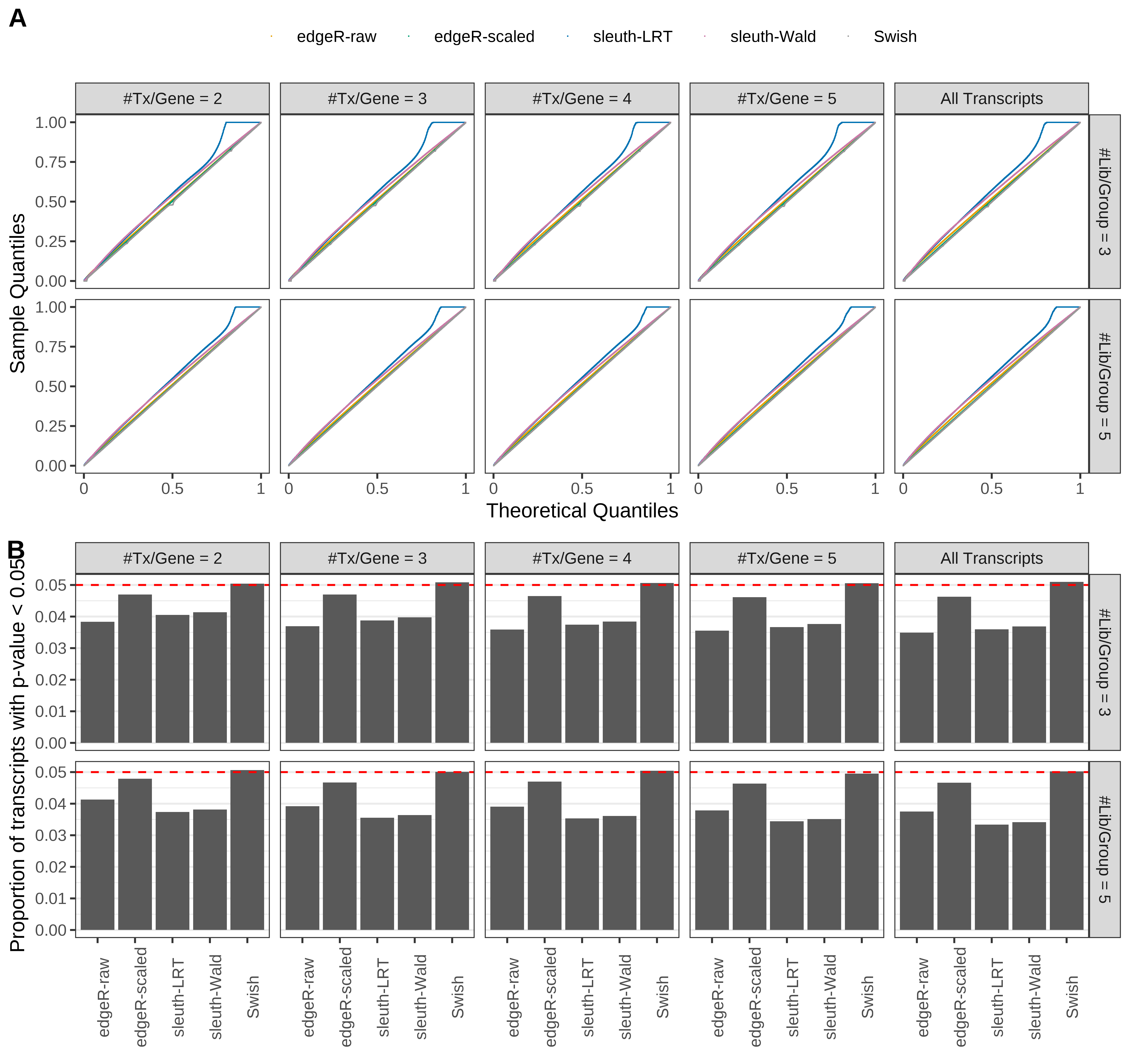
Simulation results. Scenario with mm39 genome, 125bp paired-end reads quantified with kallisto, and unbalanced libraries. (A) QQ plots of p-values for simulations without any differential expression (averaged over 20 simulations). (B) Proportion of transcripts with unadjusted p-values less than 0.05 for simulations without any differential expression (averaged over 20 simulations)

Simulation results. Scenario with mm39 genome, 150bp paired-end reads quantified with kallisto, and unbalanced libraries. (A) QQ plots of p-values for simulations without any differential expression (averaged over 20 simulations). (B) Proportion of transcripts with unadjusted p-values less than 0.05 for simulations without any differential expression (averaged over 20 simulations)
Distribution of unadjusted p-values
Distribution of unadjusted p-values from null simulations are then presented.
> for(i in seq_len(length(plots))) {
+   fig <- plots[[i]]$panelC
+   print(fig)
+   cat('\n\n<!-- -->\n\n')
+ } 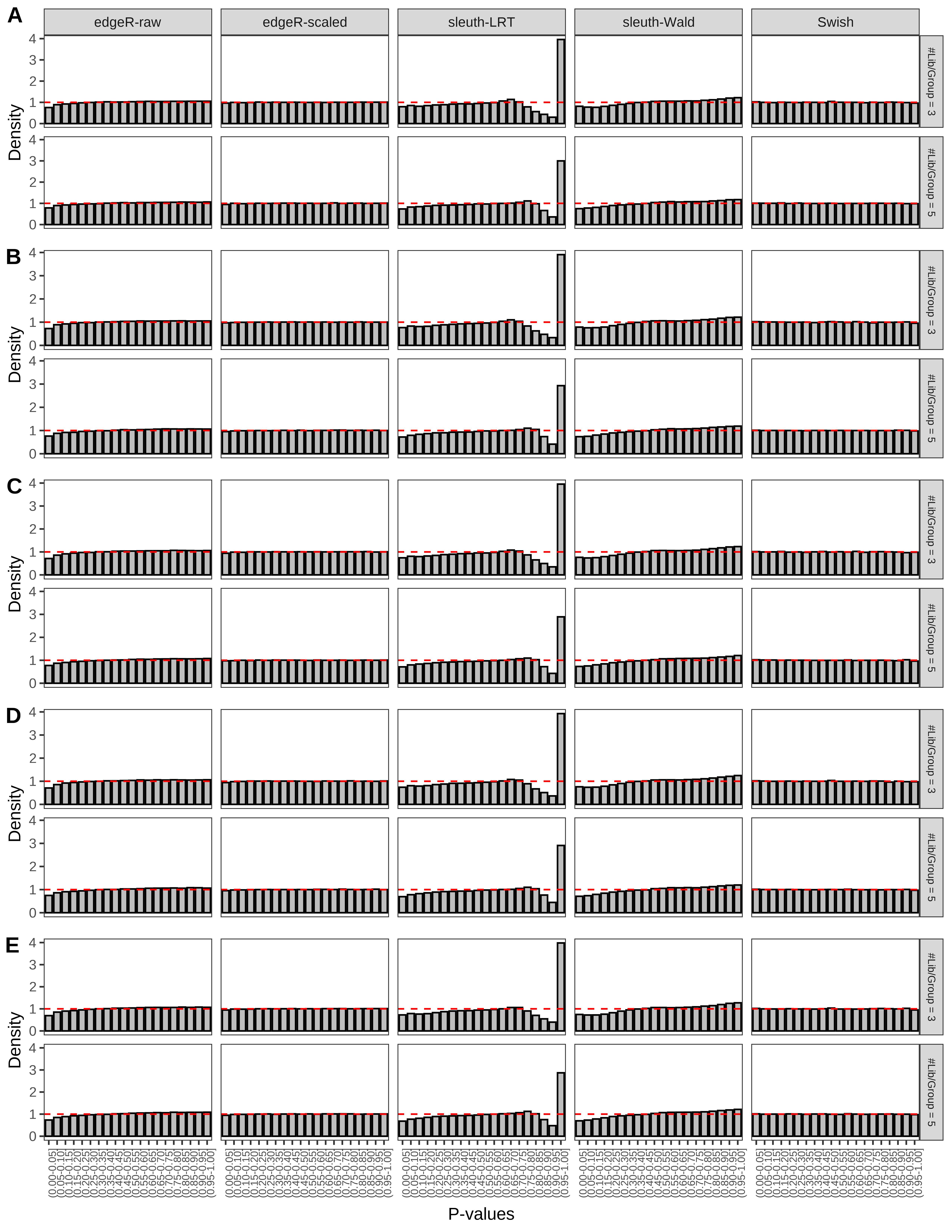
Simulation results. Scenario with mm39 genome, 50bp single-end reads quantified with Salmon, and balanced libraries. (A) Density histograms for simulations without any differential expression (averaged over 20 simulations).

Simulation results. Scenario with mm39 genome, 75bp single-end reads quantified with Salmon, and balanced libraries. (A) Density histograms for simulations without any differential expression (averaged over 20 simulations).
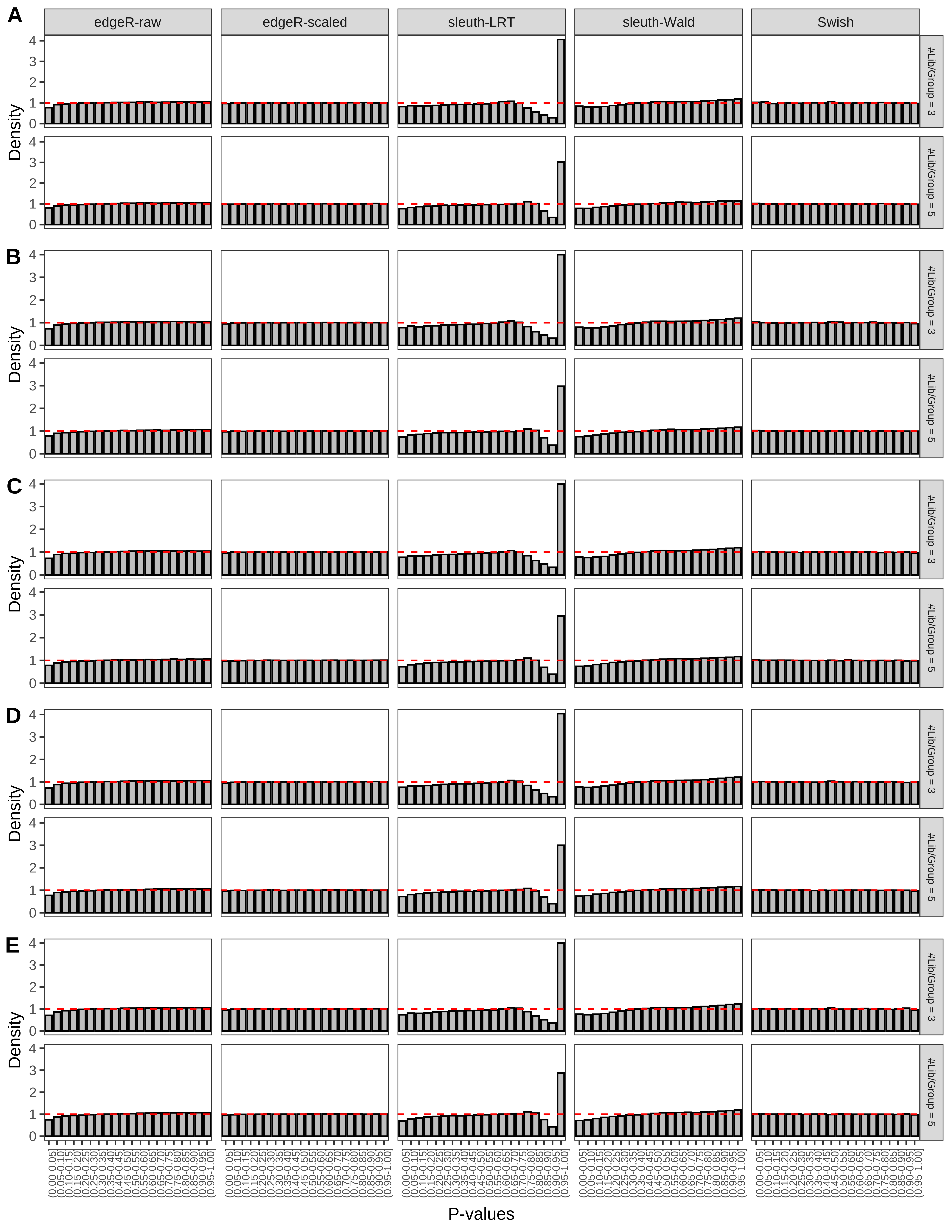
Simulation results. Scenario with mm39 genome, 100bp single-end reads quantified with Salmon, and balanced libraries. (A) Density histograms for simulations without any differential expression (averaged over 20 simulations).
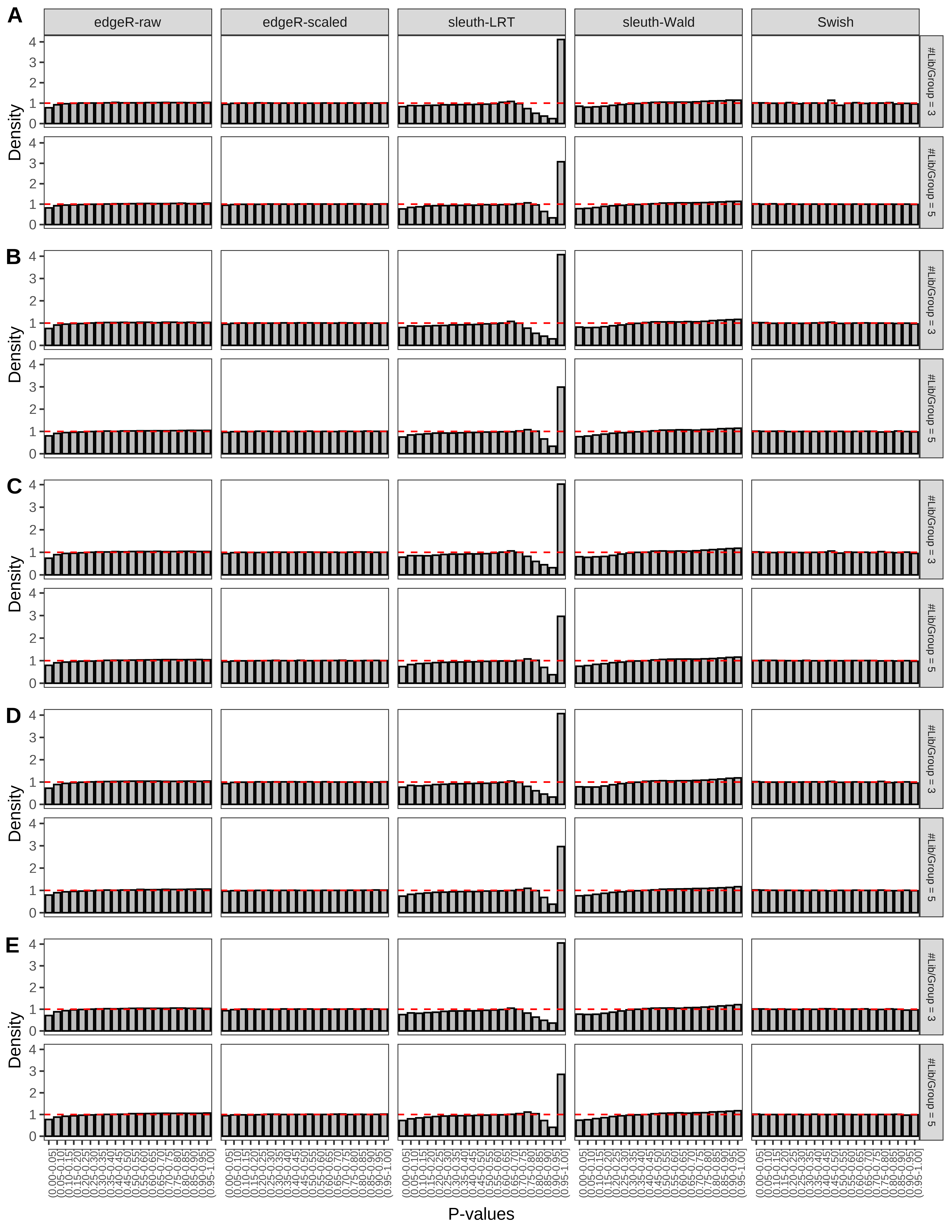
Simulation results. Scenario with mm39 genome, 125bp single-end reads quantified with Salmon, and balanced libraries. (A) Density histograms for simulations without any differential expression (averaged over 20 simulations).

Simulation results. Scenario with mm39 genome, 150bp single-end reads quantified with Salmon, and balanced libraries. (A) Density histograms for simulations without any differential expression (averaged over 20 simulations).

Simulation results. Scenario with mm39 genome, 50bp paired-end reads quantified with Salmon, and balanced libraries. (A) Density histograms for simulations without any differential expression (averaged over 20 simulations).

Simulation results. Scenario with mm39 genome, 75bp paired-end reads quantified with Salmon, and balanced libraries. (A) Density histograms for simulations without any differential expression (averaged over 20 simulations).

Simulation results. Scenario with mm39 genome, 100bp paired-end reads quantified with Salmon, and balanced libraries. (A) Density histograms for simulations without any differential expression (averaged over 20 simulations).

Simulation results. Scenario with mm39 genome, 125bp paired-end reads quantified with Salmon, and balanced libraries. (A) Density histograms for simulations without any differential expression (averaged over 20 simulations).

Simulation results. Scenario with mm39 genome, 150bp paired-end reads quantified with Salmon, and balanced libraries. (A) Density histograms for simulations without any differential expression (averaged over 20 simulations).

Simulation results. Scenario with mm39 genome, 50bp single-end reads quantified with kallisto, and balanced libraries. (A) Density histograms for simulations without any differential expression (averaged over 20 simulations).
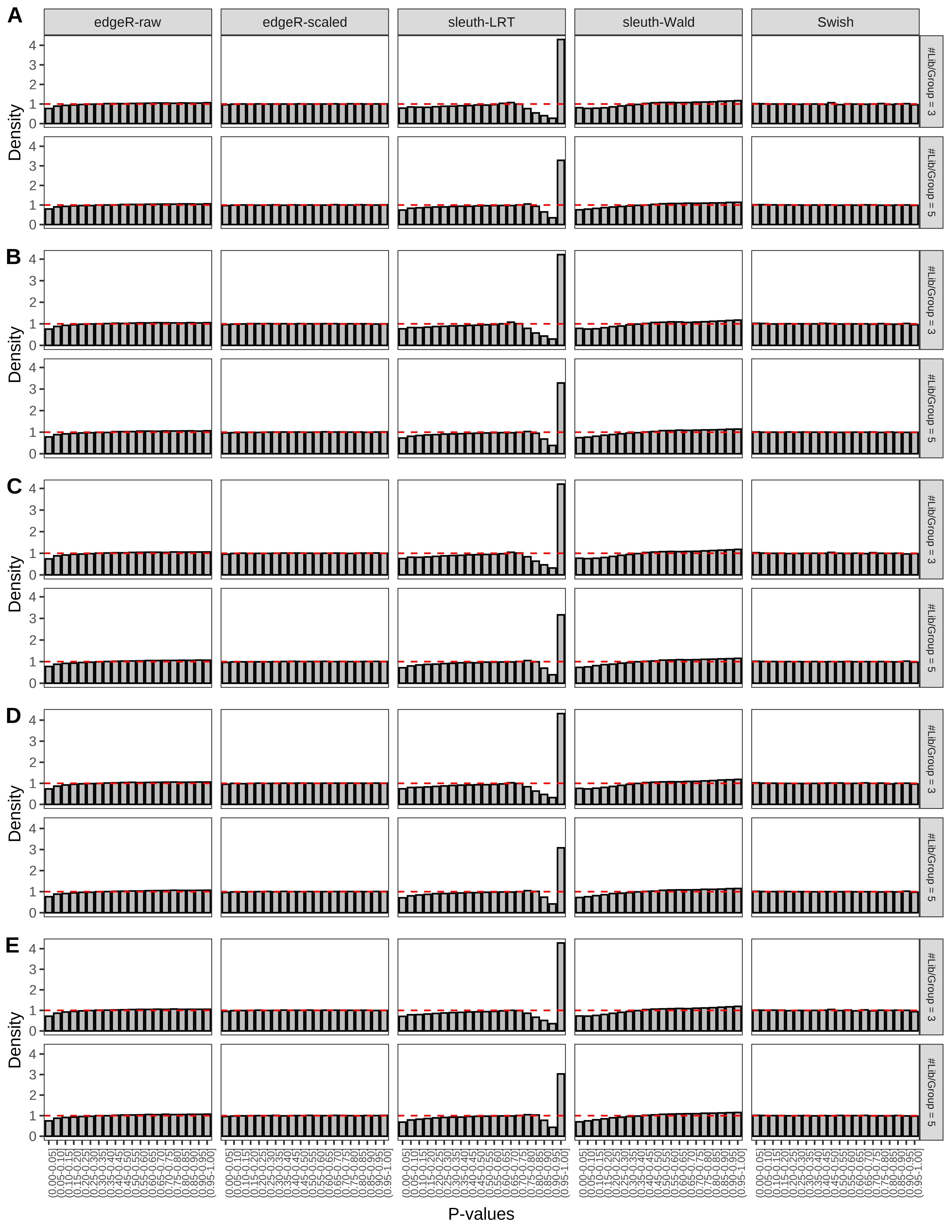
Simulation results. Scenario with mm39 genome, 75bp single-end reads quantified with kallisto, and balanced libraries. (A) Density histograms for simulations without any differential expression (averaged over 20 simulations).

Simulation results. Scenario with mm39 genome, 100bp single-end reads quantified with kallisto, and balanced libraries. (A) Density histograms for simulations without any differential expression (averaged over 20 simulations).
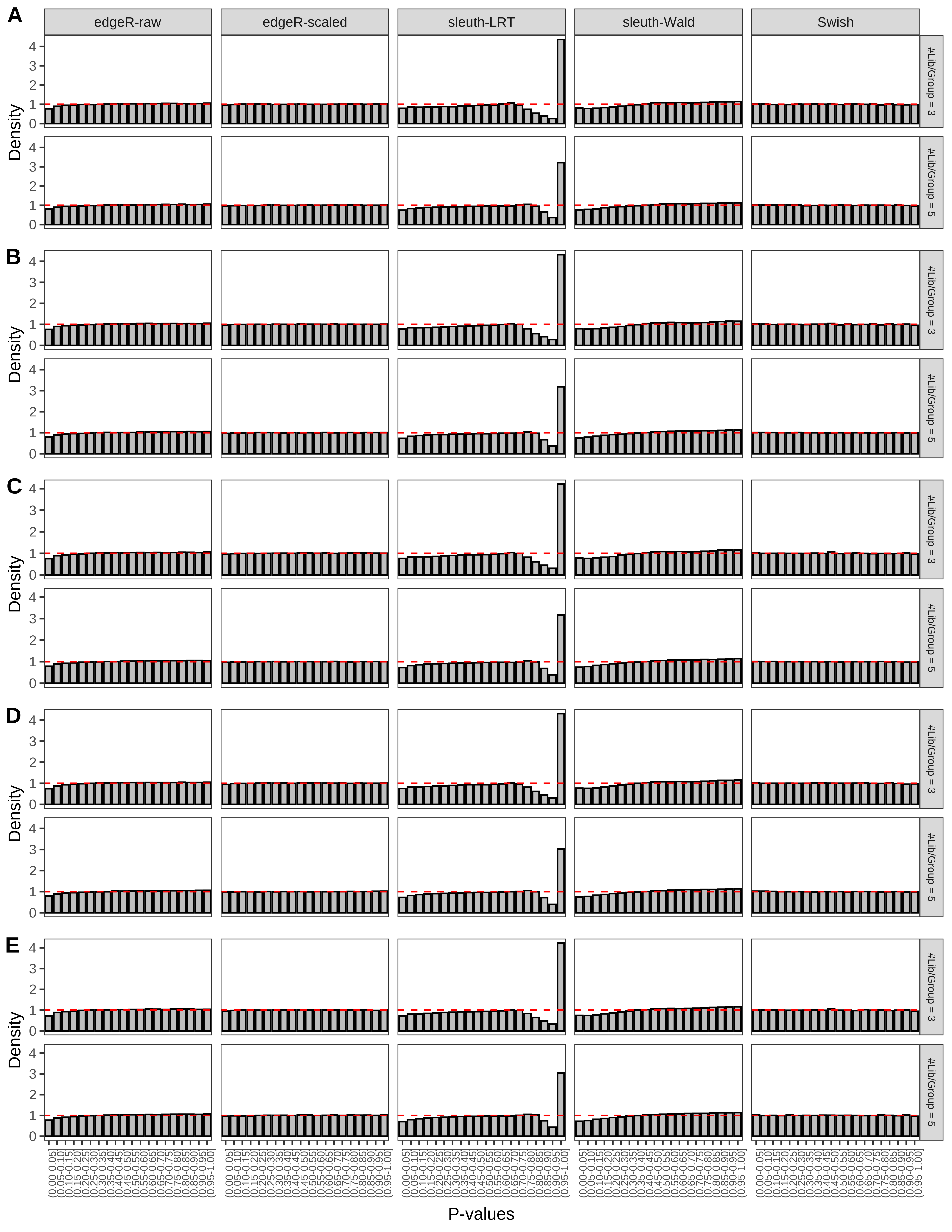
Simulation results. Scenario with mm39 genome, 125bp single-end reads quantified with kallisto, and balanced libraries. (A) Density histograms for simulations without any differential expression (averaged over 20 simulations).
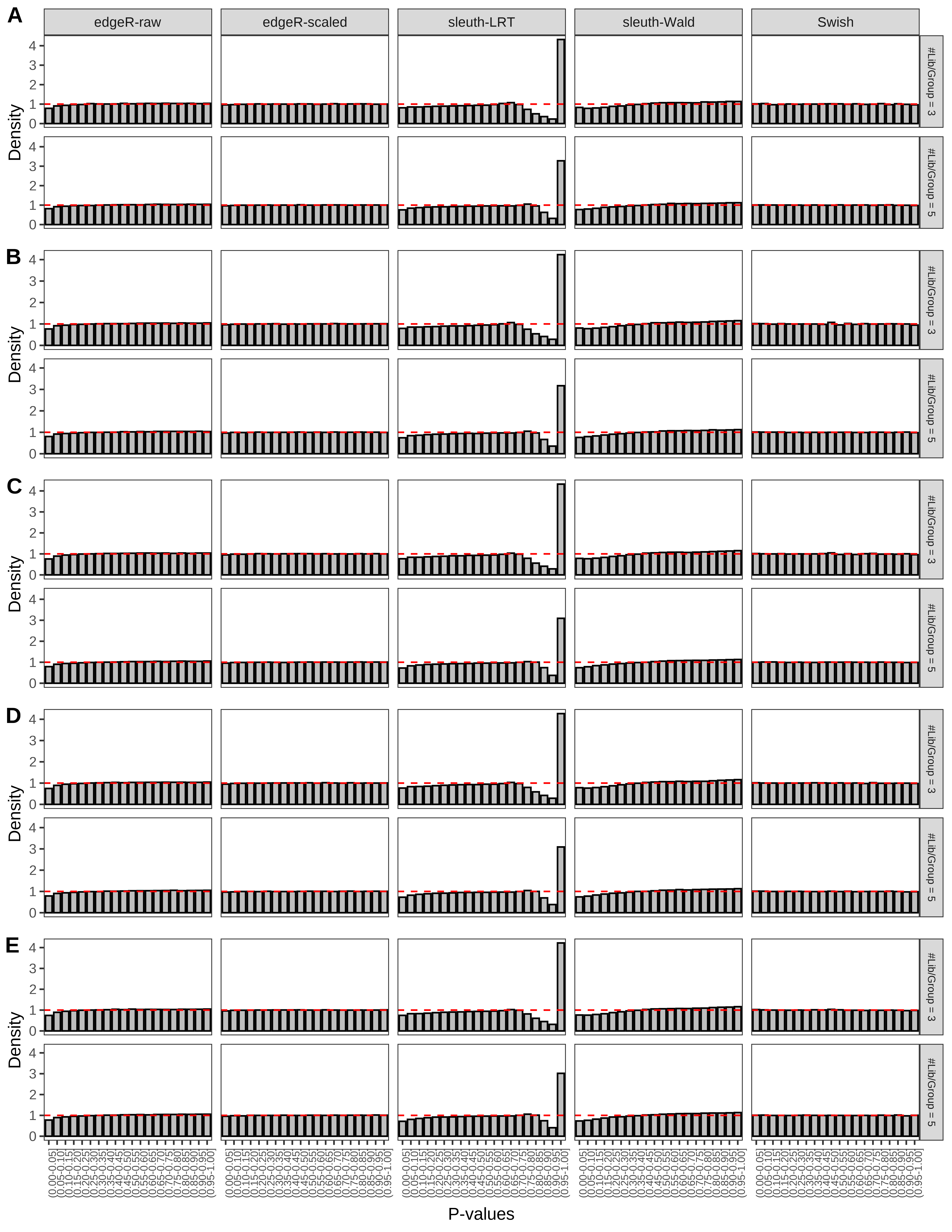
Simulation results. Scenario with mm39 genome, 150bp single-end reads quantified with kallisto, and balanced libraries. (A) Density histograms for simulations without any differential expression (averaged over 20 simulations).
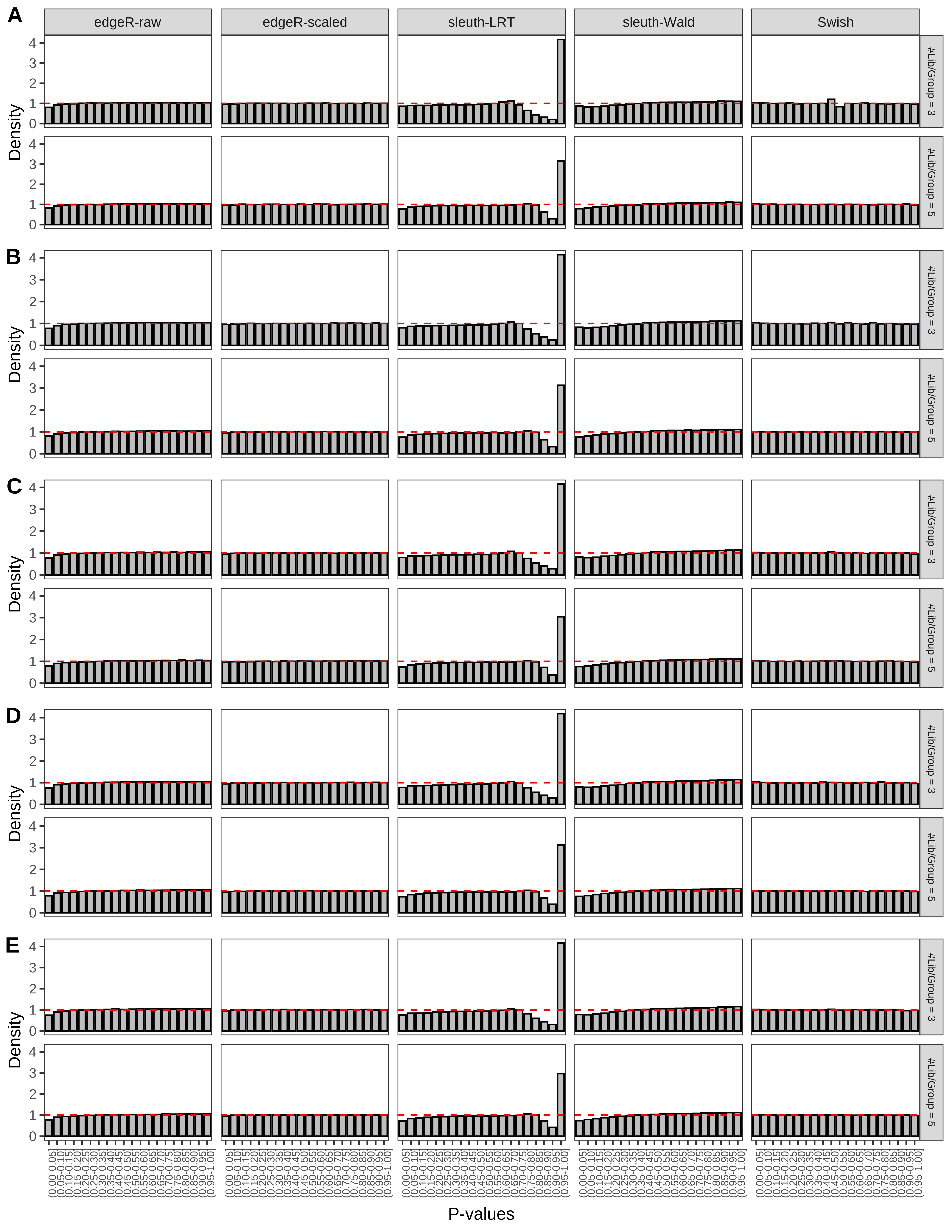
Simulation results. Scenario with mm39 genome, 50bp paired-end reads quantified with kallisto, and balanced libraries. (A) Density histograms for simulations without any differential expression (averaged over 20 simulations).

Simulation results. Scenario with mm39 genome, 75bp paired-end reads quantified with kallisto, and balanced libraries. (A) Density histograms for simulations without any differential expression (averaged over 20 simulations).

Simulation results. Scenario with mm39 genome, 100bp paired-end reads quantified with kallisto, and balanced libraries. (A) Density histograms for simulations without any differential expression (averaged over 20 simulations).

Simulation results. Scenario with mm39 genome, 125bp paired-end reads quantified with kallisto, and balanced libraries. (A) Density histograms for simulations without any differential expression (averaged over 20 simulations).
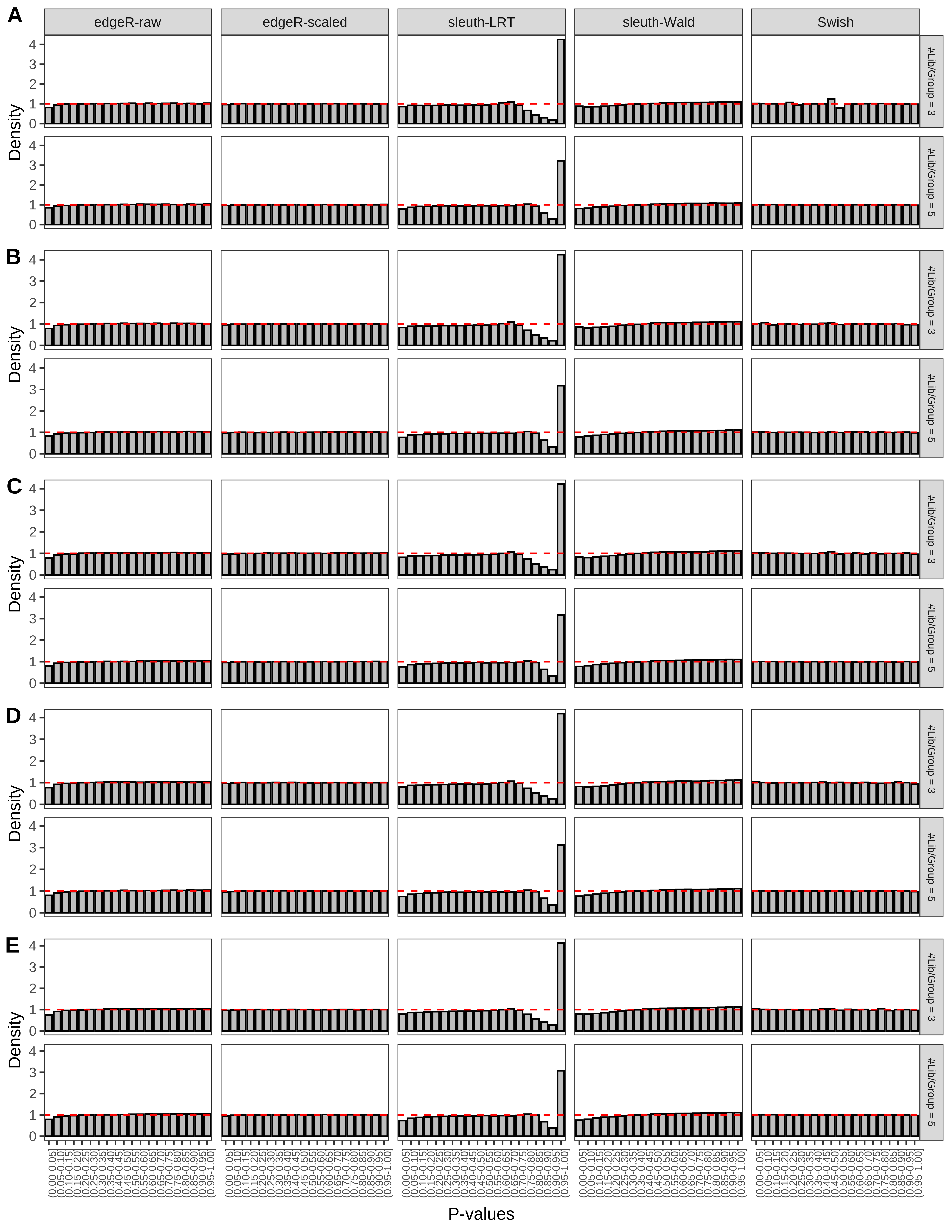
Simulation results. Scenario with mm39 genome, 150bp paired-end reads quantified with kallisto, and balanced libraries. (A) Density histograms for simulations without any differential expression (averaged over 20 simulations).
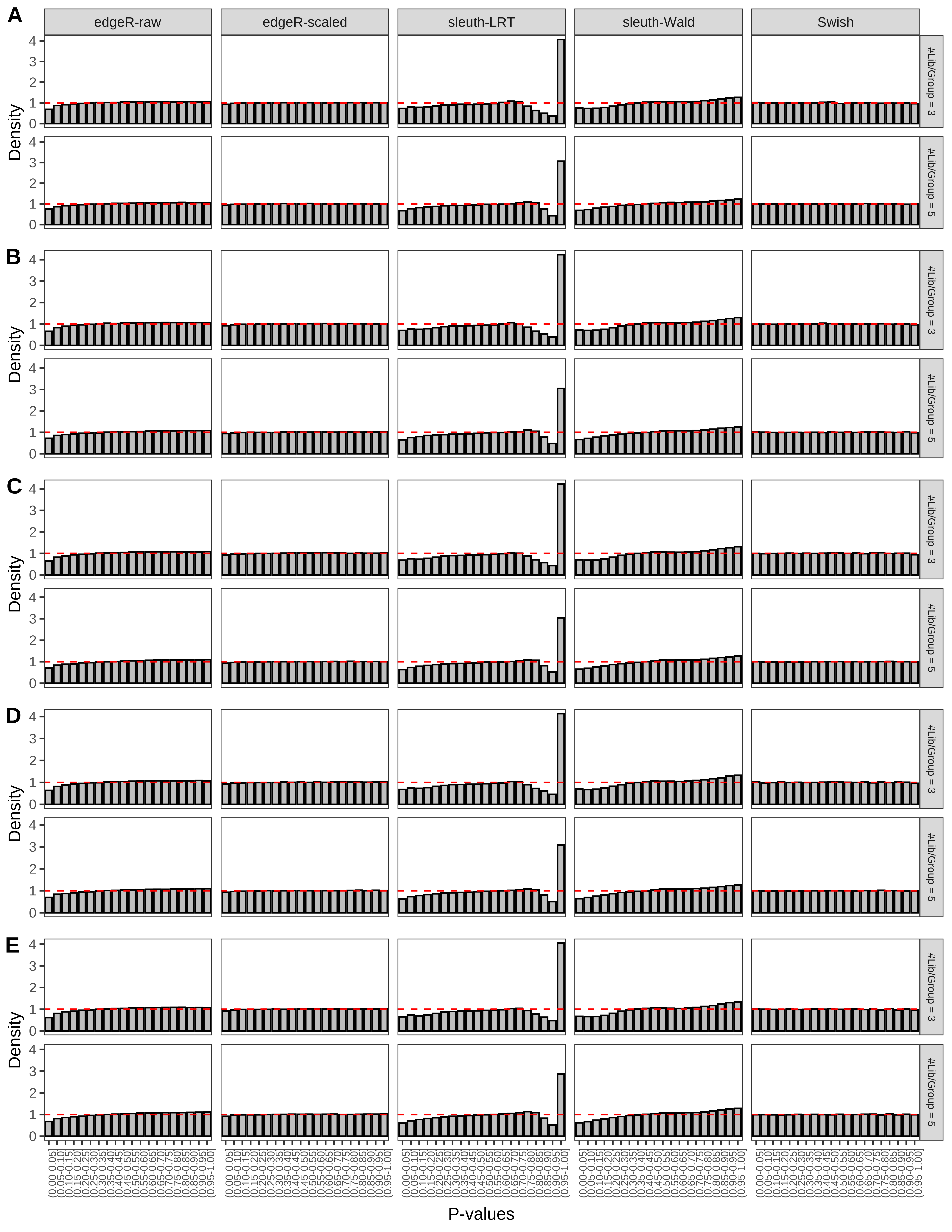
Simulation results. Scenario with mm39 genome, 50bp single-end reads quantified with Salmon, and unbalanced libraries. (A) Density histograms for simulations without any differential expression (averaged over 20 simulations).

Simulation results. Scenario with mm39 genome, 75bp single-end reads quantified with Salmon, and unbalanced libraries. (A) Density histograms for simulations without any differential expression (averaged over 20 simulations).

Simulation results. Scenario with mm39 genome, 100bp single-end reads quantified with Salmon, and unbalanced libraries. (A) Density histograms for simulations without any differential expression (averaged over 20 simulations).

Simulation results. Scenario with mm39 genome, 125bp single-end reads quantified with Salmon, and unbalanced libraries. (A) Density histograms for simulations without any differential expression (averaged over 20 simulations).

Simulation results. Scenario with mm39 genome, 150bp single-end reads quantified with Salmon, and unbalanced libraries. (A) Density histograms for simulations without any differential expression (averaged over 20 simulations).
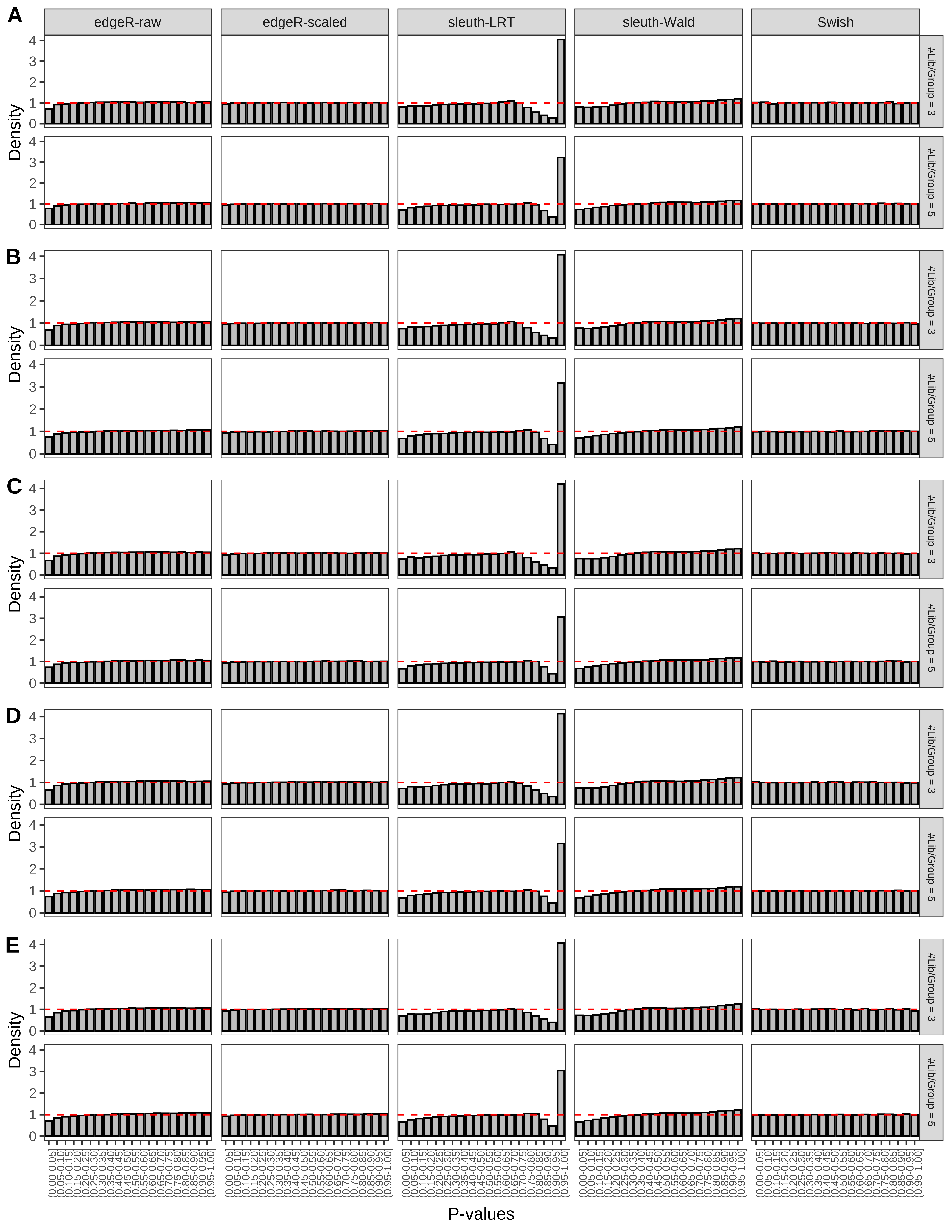
Simulation results. Scenario with mm39 genome, 50bp paired-end reads quantified with Salmon, and unbalanced libraries. (A) Density histograms for simulations without any differential expression (averaged over 20 simulations).

Simulation results. Scenario with mm39 genome, 75bp paired-end reads quantified with Salmon, and unbalanced libraries. (A) Density histograms for simulations without any differential expression (averaged over 20 simulations).

Simulation results. Scenario with mm39 genome, 100bp paired-end reads quantified with Salmon, and unbalanced libraries. (A) Density histograms for simulations without any differential expression (averaged over 20 simulations).

Simulation results. Scenario with mm39 genome, 125bp paired-end reads quantified with Salmon, and unbalanced libraries. (A) Density histograms for simulations without any differential expression (averaged over 20 simulations).

Simulation results. Scenario with mm39 genome, 150bp paired-end reads quantified with Salmon, and unbalanced libraries. (A) Density histograms for simulations without any differential expression (averaged over 20 simulations).

Simulation results. Scenario with mm39 genome, 50bp single-end reads quantified with kallisto, and unbalanced libraries. (A) Density histograms for simulations without any differential expression (averaged over 20 simulations).
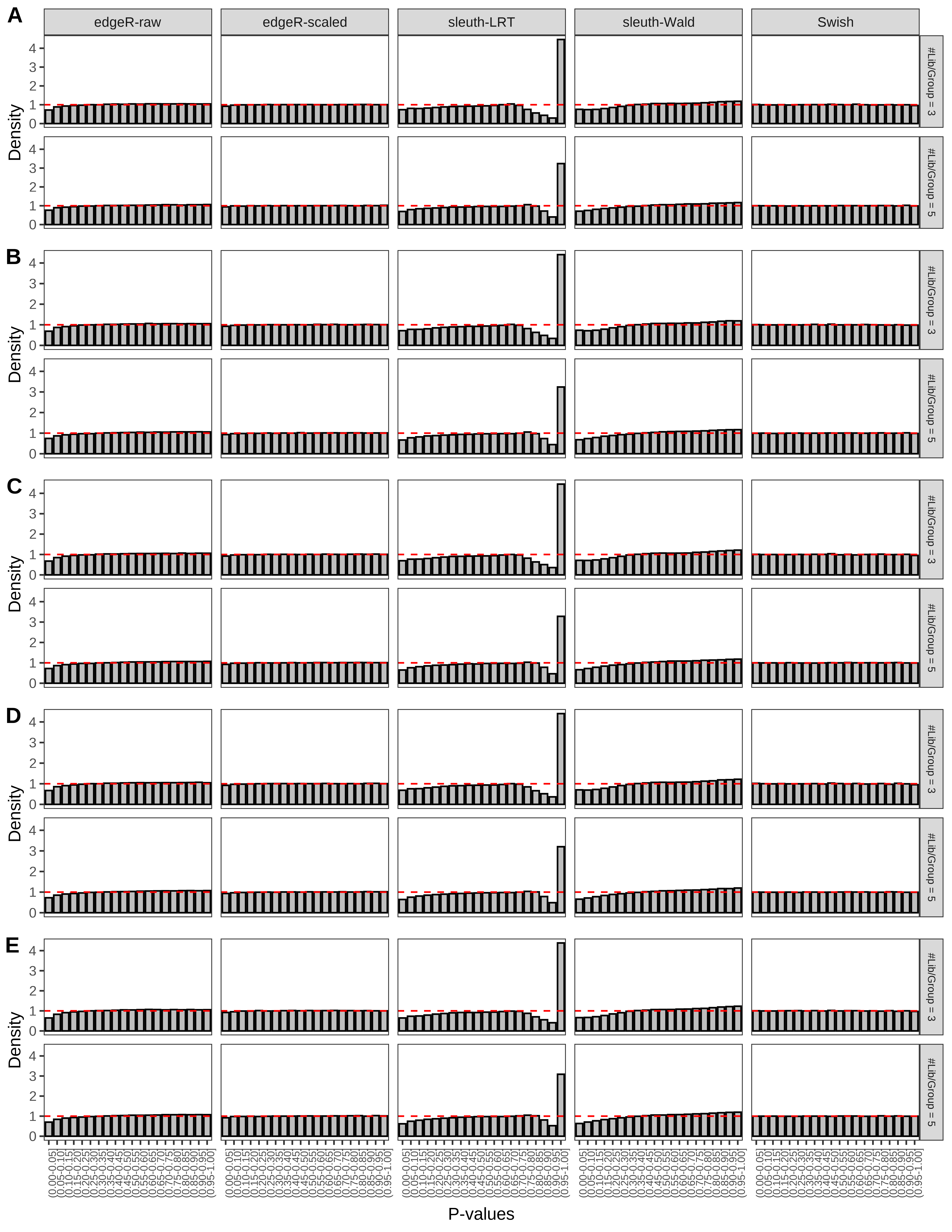
Simulation results. Scenario with mm39 genome, 75bp single-end reads quantified with kallisto, and unbalanced libraries. (A) Density histograms for simulations without any differential expression (averaged over 20 simulations).

Simulation results. Scenario with mm39 genome, 100bp single-end reads quantified with kallisto, and unbalanced libraries. (A) Density histograms for simulations without any differential expression (averaged over 20 simulations).

Simulation results. Scenario with mm39 genome, 125bp single-end reads quantified with kallisto, and unbalanced libraries. (A) Density histograms for simulations without any differential expression (averaged over 20 simulations).
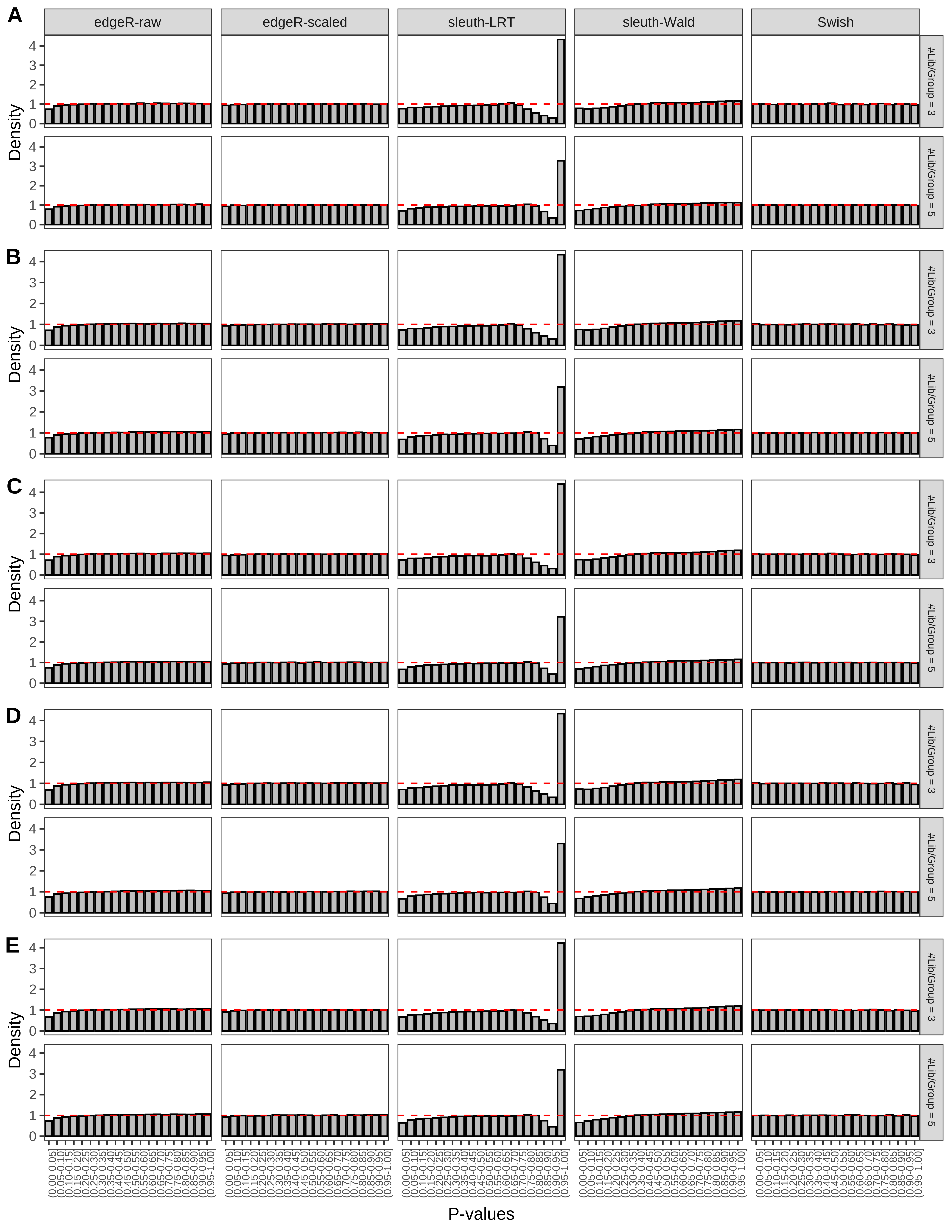
Simulation results. Scenario with mm39 genome, 150bp single-end reads quantified with kallisto, and unbalanced libraries. (A) Density histograms for simulations without any differential expression (averaged over 20 simulations).
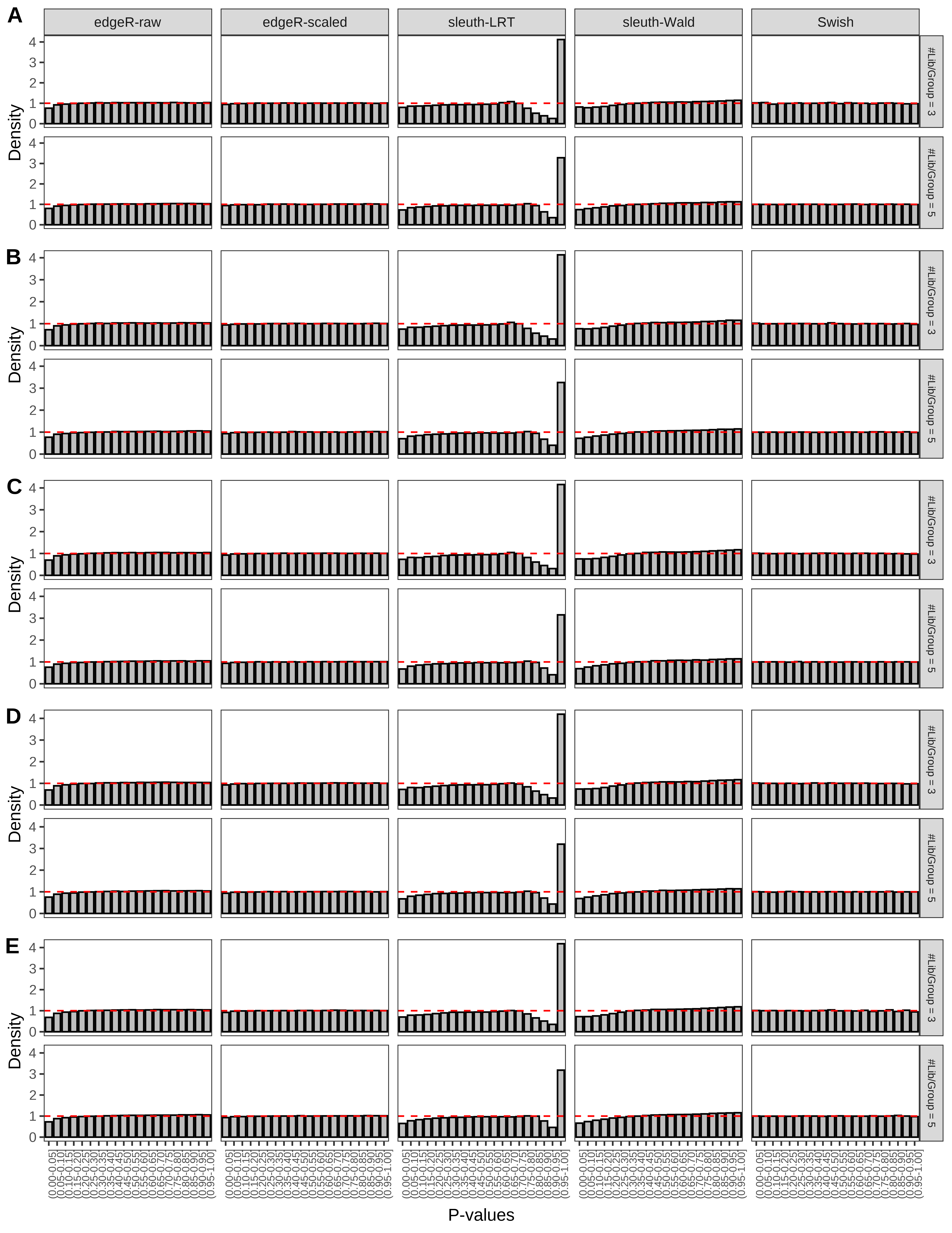
Simulation results. Scenario with mm39 genome, 50bp paired-end reads quantified with kallisto, and unbalanced libraries. (A) Density histograms for simulations without any differential expression (averaged over 20 simulations).

Simulation results. Scenario with mm39 genome, 75bp paired-end reads quantified with kallisto, and unbalanced libraries. (A) Density histograms for simulations without any differential expression (averaged over 20 simulations).
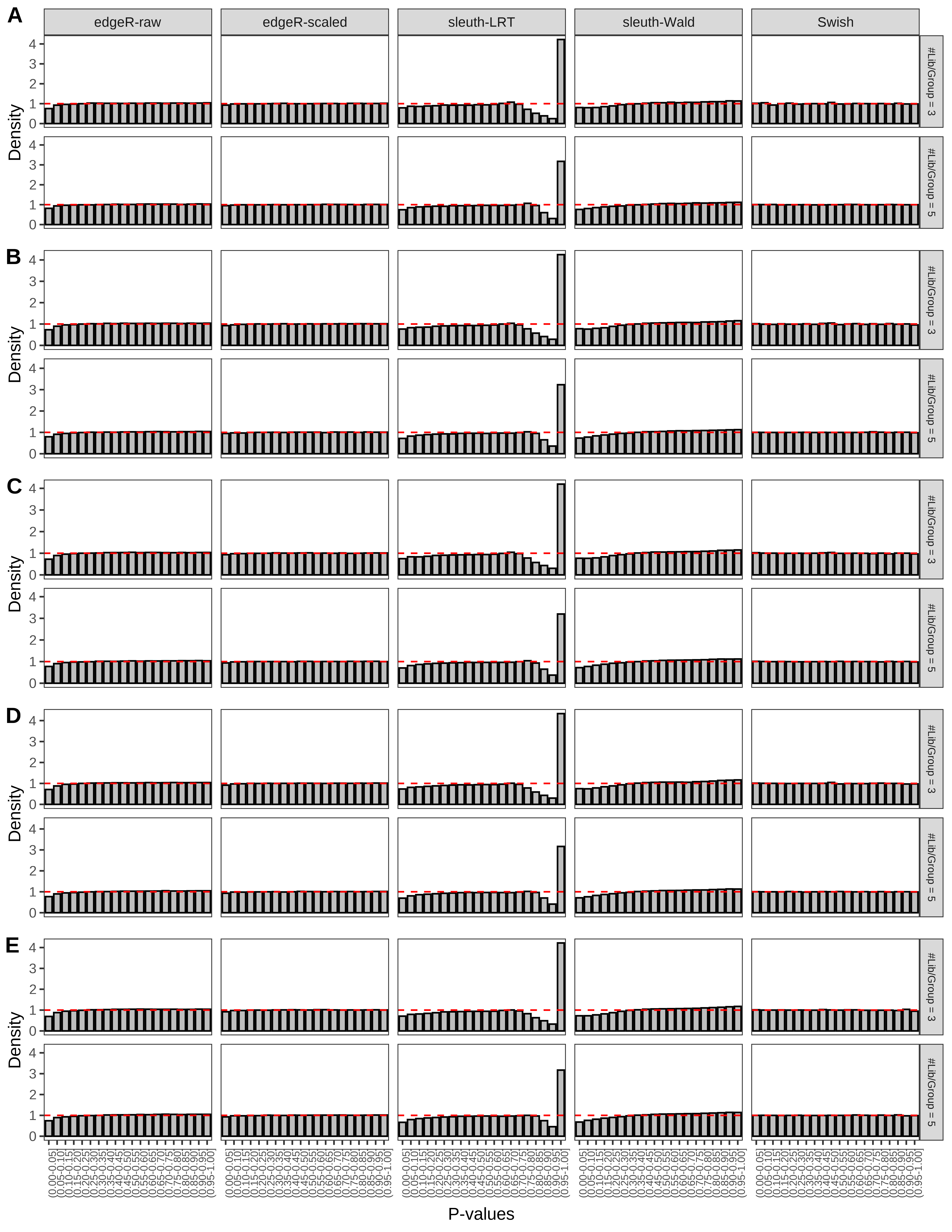
Simulation results. Scenario with mm39 genome, 100bp paired-end reads quantified with kallisto, and unbalanced libraries. (A) Density histograms for simulations without any differential expression (averaged over 20 simulations).

Simulation results. Scenario with mm39 genome, 125bp paired-end reads quantified with kallisto, and unbalanced libraries. (A) Density histograms for simulations without any differential expression (averaged over 20 simulations).
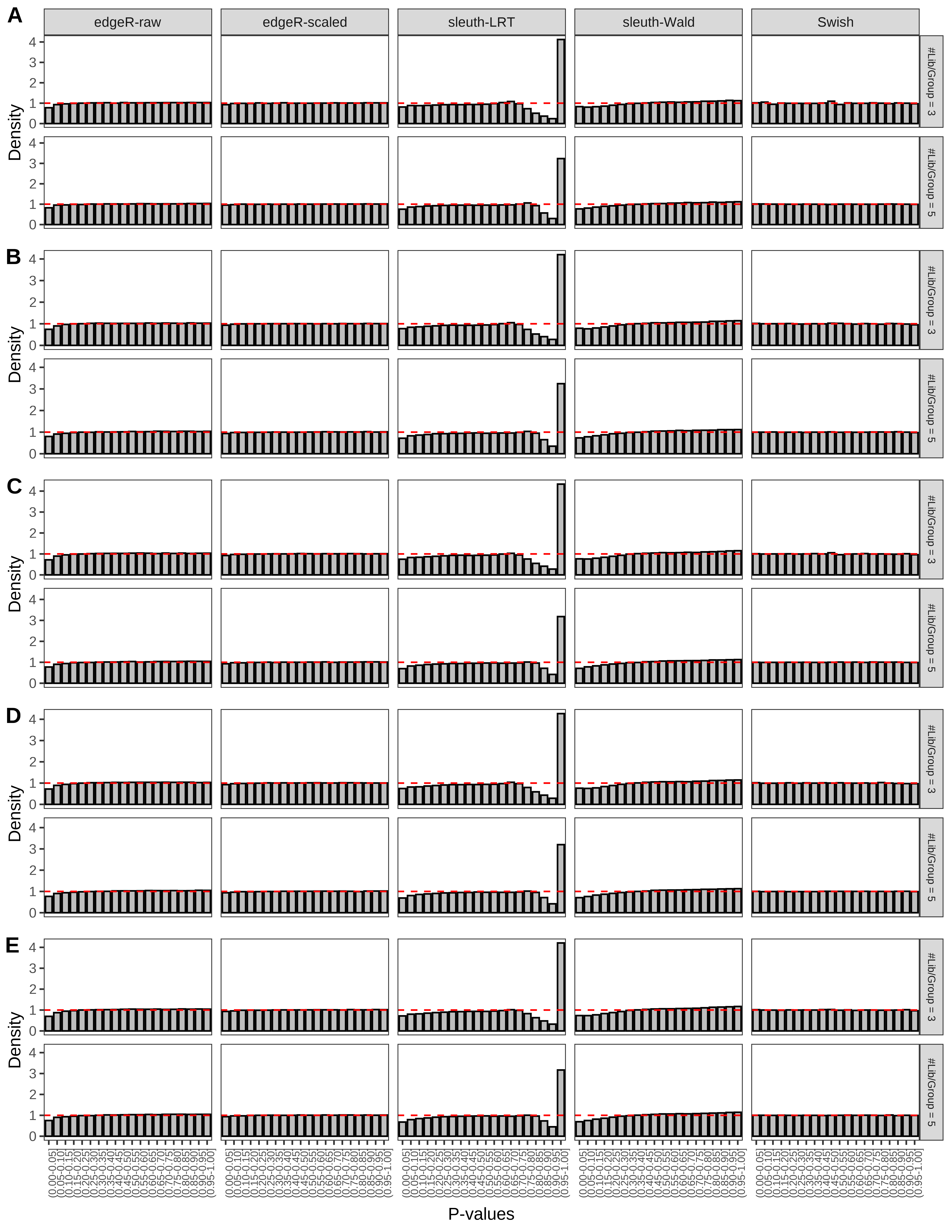
Simulation results. Scenario with mm39 genome, 150bp paired-end reads quantified with kallisto, and unbalanced libraries. (A) Density histograms for simulations without any differential expression (averaged over 20 simulations).
Power and false discovery rate by read lengths
Finally, tables assessing power and FDR by different read length specifications are presented.
> for(i in seq_len(length(tables))) {
+   tb <- tables[[i]]$table1
+   print(tb)
+   cat('\n\n<!-- -->\n\n')
+ } | Read | Samples/Group | Library Size | Read Length | edgeR-raw | edgeR-scaled | sleuth-LRT | sleuth-Wald | Swish | edgeR-raw | edgeR-scaled | sleuth-LRT | sleuth-Wald | Swish |
|---|---|---|---|---|---|---|---|---|---|---|---|---|---|
| paired-end | 3 | 50M | 50bp | 0.211 | 0.513 | 0.171 | 0.461 | 0.483 | 0.057 | 0.041 | 0.011 | 0.057 | 0.215 |
| paired-end | 3 | 50M | 75bp | 0.304 | 0.522 | 0.197 | 0.475 | 0.486 | 0.028 | 0.039 | 0.011 | 0.054 | 0.211 |
| paired-end | 3 | 50M | 100bp | 0.298 | 0.517 | 0.189 | 0.467 | 0.476 | 0.030 | 0.039 | 0.011 | 0.054 | 0.208 |
| paired-end | 3 | 50M | 125bp | 0.326 | 0.522 | 0.199 | 0.477 | 0.492 | 0.025 | 0.038 | 0.009 | 0.053 | 0.215 |
| paired-end | 3 | 50M | 150bp | 0.320 | 0.525 | 0.204 | 0.478 | 0.494 | 0.024 | 0.038 | 0.011 | 0.055 | 0.213 |
| paired-end | 3 | 25/100M | 50bp | 0.127 | 0.464 | 0.076 | 0.405 | 0.428 | 0.043 | 0.036 | 0.003 | 0.045 | 0.199 |
| paired-end | 3 | 25/100M | 75bp | 0.206 | 0.466 | 0.111 | 0.411 | 0.430 | 0.020 | 0.035 | 0.006 | 0.046 | 0.199 |
| paired-end | 3 | 25/100M | 100bp | 0.201 | 0.463 | 0.104 | 0.407 | 0.423 | 0.021 | 0.034 | 0.005 | 0.046 | 0.194 |
| paired-end | 3 | 25/100M | 125bp | 0.232 | 0.478 | 0.129 | 0.424 | 0.437 | 0.023 | 0.039 | 0.007 | 0.050 | 0.203 |
| paired-end | 3 | 25/100M | 150bp | 0.224 | 0.467 | 0.099 | 0.414 | 0.434 | 0.021 | 0.037 | 0.007 | 0.050 | 0.205 |
| paired-end | 5 | 50M | 50bp | 0.655 | 0.756 | 0.626 | 0.688 | 0.500 | 0.029 | 0.044 | 0.026 | 0.042 | 0.043 |
| paired-end | 5 | 50M | 75bp | 0.687 | 0.761 | 0.636 | 0.697 | 0.503 | 0.028 | 0.041 | 0.025 | 0.040 | 0.044 |
| paired-end | 5 | 50M | 100bp | 0.687 | 0.758 | 0.636 | 0.696 | 0.518 | 0.026 | 0.040 | 0.024 | 0.038 | 0.045 |
| paired-end | 5 | 50M | 125bp | 0.701 | 0.766 | 0.648 | 0.707 | 0.485 | 0.027 | 0.039 | 0.024 | 0.038 | 0.038 |
| paired-end | 5 | 50M | 150bp | 0.693 | 0.761 | 0.643 | 0.703 | 0.505 | 0.026 | 0.039 | 0.024 | 0.038 | 0.044 |
| paired-end | 5 | 25/100M | 50bp | 0.604 | 0.716 | 0.567 | 0.630 | 0.478 | 0.023 | 0.039 | 0.021 | 0.037 | 0.045 |
| paired-end | 5 | 25/100M | 75bp | 0.638 | 0.724 | 0.581 | 0.645 | 0.474 | 0.024 | 0.038 | 0.022 | 0.035 | 0.044 |
| paired-end | 5 | 25/100M | 100bp | 0.635 | 0.719 | 0.578 | 0.639 | 0.465 | 0.024 | 0.039 | 0.022 | 0.036 | 0.041 |
| paired-end | 5 | 25/100M | 125bp | 0.647 | 0.728 | 0.587 | 0.653 | 0.461 | 0.024 | 0.039 | 0.022 | 0.037 | 0.042 |
| paired-end | 5 | 25/100M | 150bp | 0.645 | 0.726 | 0.587 | 0.648 | 0.473 | 0.025 | 0.039 | 0.021 | 0.036 | 0.043 |
| single-end | 3 | 50M | 50bp | 0.126 | 0.484 | 0.146 | 0.430 | 0.455 | 0.088 | 0.049 | 0.019 | 0.063 | 0.216 |
| single-end | 3 | 50M | 75bp | 0.173 | 0.493 | 0.156 | 0.439 | 0.462 | 0.070 | 0.047 | 0.016 | 0.059 | 0.210 |
| single-end | 3 | 50M | 100bp | 0.187 | 0.496 | 0.159 | 0.438 | 0.460 | 0.068 | 0.046 | 0.018 | 0.059 | 0.213 |
| single-end | 3 | 50M | 125bp | 0.234 | 0.497 | 0.176 | 0.456 | 0.478 | 0.052 | 0.042 | 0.014 | 0.059 | 0.217 |
| single-end | 3 | 50M | 150bp | 0.255 | 0.499 | 0.181 | 0.458 | 0.479 | 0.044 | 0.041 | 0.015 | 0.057 | 0.215 |
| single-end | 3 | 25/100M | 50bp | 0.012 | 0.430 | 0.030 | 0.366 | 0.399 | 0.116 | 0.041 | 0.009 | 0.052 | 0.203 |
| single-end | 3 | 25/100M | 75bp | 0.029 | 0.438 | 0.026 | 0.380 | 0.409 | 0.073 | 0.040 | 0.014 | 0.053 | 0.195 |
| single-end | 3 | 25/100M | 100bp | 0.099 | 0.443 | 0.067 | 0.383 | 0.409 | 0.055 | 0.037 | 0.007 | 0.048 | 0.196 |
| single-end | 3 | 25/100M | 125bp | 0.136 | 0.447 | 0.077 | 0.394 | 0.420 | 0.043 | 0.038 | 0.009 | 0.052 | 0.202 |
| single-end | 3 | 25/100M | 150bp | 0.175 | 0.460 | 0.098 | 0.406 | 0.428 | 0.035 | 0.038 | 0.008 | 0.050 | 0.205 |
| single-end | 5 | 50M | 50bp | 0.602 | 0.725 | 0.579 | 0.641 | 0.483 | 0.045 | 0.058 | 0.039 | 0.053 | 0.056 |
| single-end | 5 | 50M | 75bp | 0.619 | 0.732 | 0.593 | 0.655 | 0.497 | 0.042 | 0.055 | 0.036 | 0.051 | 0.059 |
| single-end | 5 | 50M | 100bp | 0.630 | 0.739 | 0.602 | 0.663 | 0.473 | 0.038 | 0.052 | 0.032 | 0.048 | 0.048 |
| single-end | 5 | 50M | 125bp | 0.651 | 0.744 | 0.617 | 0.677 | 0.509 | 0.036 | 0.047 | 0.033 | 0.048 | 0.054 |
| single-end | 5 | 50M | 150bp | 0.665 | 0.753 | 0.628 | 0.691 | 0.507 | 0.033 | 0.046 | 0.031 | 0.046 | 0.051 |
| single-end | 5 | 25/100M | 50bp | 0.554 | 0.685 | 0.522 | 0.583 | 0.449 | 0.037 | 0.051 | 0.031 | 0.047 | 0.052 |
| single-end | 5 | 25/100M | 75bp | 0.565 | 0.694 | 0.527 | 0.591 | 0.455 | 0.035 | 0.047 | 0.029 | 0.044 | 0.054 |
| single-end | 5 | 25/100M | 100bp | 0.573 | 0.691 | 0.533 | 0.596 | 0.450 | 0.033 | 0.046 | 0.027 | 0.043 | 0.051 |
| single-end | 5 | 25/100M | 125bp | 0.602 | 0.709 | 0.556 | 0.620 | 0.464 | 0.031 | 0.045 | 0.028 | 0.042 | 0.049 |
| single-end | 5 | 25/100M | 150bp | 0.616 | 0.713 | 0.567 | 0.628 | 0.482 | 0.031 | 0.043 | 0.026 | 0.041 | 0.049 |
| Read | Samples/Group | Library Size | Read Length | edgeR-raw | edgeR-scaled | sleuth-LRT | sleuth-Wald | Swish | edgeR-raw | edgeR-scaled | sleuth-LRT | sleuth-Wald | Swish |
|---|---|---|---|---|---|---|---|---|---|---|---|---|---|
| paired-end | 3 | 50M | 50bp | 0.251 | 0.515 | 0.168 | 0.463 | 0.495 | 0.053 | 0.041 | 0.010 | 0.055 | 0.223 |
| paired-end | 3 | 50M | 75bp | 0.266 | 0.521 | 0.181 | 0.473 | 0.500 | 0.049 | 0.038 | 0.011 | 0.055 | 0.222 |
| paired-end | 3 | 50M | 100bp | 0.264 | 0.521 | 0.178 | 0.468 | 0.498 | 0.053 | 0.040 | 0.011 | 0.054 | 0.225 |
| paired-end | 3 | 50M | 125bp | 0.284 | 0.524 | 0.181 | 0.473 | 0.501 | 0.047 | 0.040 | 0.009 | 0.053 | 0.225 |
| paired-end | 3 | 50M | 150bp | 0.289 | 0.527 | 0.190 | 0.476 | 0.505 | 0.043 | 0.039 | 0.010 | 0.054 | 0.224 |
| paired-end | 3 | 25/100M | 50bp | 0.180 | 0.462 | 0.075 | 0.406 | 0.436 | 0.034 | 0.036 | 0.002 | 0.047 | 0.207 |
| paired-end | 3 | 25/100M | 75bp | 0.193 | 0.468 | 0.083 | 0.412 | 0.441 | 0.032 | 0.035 | 0.006 | 0.046 | 0.206 |
| paired-end | 3 | 25/100M | 100bp | 0.198 | 0.467 | 0.094 | 0.415 | 0.442 | 0.035 | 0.035 | 0.004 | 0.047 | 0.207 |
| paired-end | 3 | 25/100M | 125bp | 0.215 | 0.478 | 0.100 | 0.421 | 0.444 | 0.036 | 0.039 | 0.006 | 0.050 | 0.212 |
| paired-end | 3 | 25/100M | 150bp | 0.211 | 0.467 | 0.078 | 0.414 | 0.442 | 0.032 | 0.037 | 0.006 | 0.050 | 0.211 |
| paired-end | 5 | 50M | 50bp | 0.661 | 0.757 | 0.631 | 0.692 | 0.489 | 0.029 | 0.042 | 0.025 | 0.041 | 0.042 |
| paired-end | 5 | 50M | 75bp | 0.670 | 0.764 | 0.635 | 0.699 | 0.495 | 0.031 | 0.042 | 0.026 | 0.041 | 0.042 |
| paired-end | 5 | 50M | 100bp | 0.674 | 0.766 | 0.640 | 0.702 | 0.493 | 0.028 | 0.042 | 0.025 | 0.040 | 0.041 |
| paired-end | 5 | 50M | 125bp | 0.681 | 0.769 | 0.646 | 0.707 | 0.492 | 0.030 | 0.040 | 0.026 | 0.040 | 0.040 |
| paired-end | 5 | 50M | 150bp | 0.675 | 0.764 | 0.640 | 0.702 | 0.511 | 0.029 | 0.040 | 0.025 | 0.040 | 0.045 |
| paired-end | 5 | 25/100M | 50bp | 0.617 | 0.716 | 0.571 | 0.636 | 0.455 | 0.026 | 0.038 | 0.021 | 0.037 | 0.042 |
| paired-end | 5 | 25/100M | 75bp | 0.629 | 0.726 | 0.583 | 0.649 | 0.473 | 0.026 | 0.039 | 0.023 | 0.037 | 0.046 |
| paired-end | 5 | 25/100M | 100bp | 0.633 | 0.727 | 0.584 | 0.650 | 0.463 | 0.027 | 0.039 | 0.023 | 0.037 | 0.043 |
| paired-end | 5 | 25/100M | 125bp | 0.639 | 0.730 | 0.586 | 0.653 | 0.479 | 0.027 | 0.039 | 0.023 | 0.037 | 0.046 |
| paired-end | 5 | 25/100M | 150bp | 0.639 | 0.728 | 0.588 | 0.650 | 0.476 | 0.028 | 0.039 | 0.022 | 0.037 | 0.044 |
| single-end | 3 | 50M | 50bp | 0.070 | 0.491 | 0.081 | 0.429 | 0.464 | 0.130 | 0.051 | 0.012 | 0.061 | 0.224 |
| single-end | 3 | 50M | 75bp | 0.124 | 0.500 | 0.115 | 0.438 | 0.473 | 0.103 | 0.050 | 0.013 | 0.059 | 0.219 |
| single-end | 3 | 50M | 100bp | 0.120 | 0.502 | 0.085 | 0.437 | 0.476 | 0.103 | 0.051 | 0.015 | 0.062 | 0.224 |
| single-end | 3 | 50M | 125bp | 0.146 | 0.503 | 0.114 | 0.447 | 0.486 | 0.093 | 0.049 | 0.012 | 0.059 | 0.225 |
| single-end | 3 | 50M | 150bp | 0.185 | 0.507 | 0.141 | 0.452 | 0.487 | 0.075 | 0.047 | 0.010 | 0.057 | 0.224 |
| single-end | 3 | 25/100M | 50bp | 0.008 | 0.434 | 0.000 | 0.369 | 0.403 | 0.133 | 0.042 | - | 0.049 | 0.208 |
| single-end | 3 | 25/100M | 75bp | 0.025 | 0.446 | 0.004 | 0.384 | 0.415 | 0.113 | 0.043 | 0.012 | 0.052 | 0.205 |
| single-end | 3 | 25/100M | 100bp | 0.065 | 0.451 | 0.010 | 0.385 | 0.420 | 0.075 | 0.038 | 0.007 | 0.049 | 0.203 |
| single-end | 3 | 25/100M | 125bp | 0.083 | 0.448 | 0.008 | 0.390 | 0.424 | 0.070 | 0.042 | 0.002 | 0.054 | 0.209 |
| single-end | 3 | 25/100M | 150bp | 0.133 | 0.463 | 0.037 | 0.402 | 0.434 | 0.051 | 0.041 | 0.006 | 0.051 | 0.211 |
| single-end | 5 | 50M | 50bp | 0.593 | 0.734 | 0.583 | 0.650 | 0.487 | 0.042 | 0.060 | 0.037 | 0.054 | 0.058 |
| single-end | 5 | 50M | 75bp | 0.611 | 0.741 | 0.597 | 0.663 | 0.512 | 0.042 | 0.060 | 0.037 | 0.054 | 0.062 |
| single-end | 5 | 50M | 100bp | 0.621 | 0.749 | 0.604 | 0.673 | 0.492 | 0.040 | 0.058 | 0.036 | 0.053 | 0.054 |
| single-end | 5 | 50M | 125bp | 0.632 | 0.752 | 0.611 | 0.679 | 0.484 | 0.040 | 0.056 | 0.036 | 0.053 | 0.052 |
| single-end | 5 | 50M | 150bp | 0.645 | 0.761 | 0.623 | 0.692 | 0.496 | 0.039 | 0.056 | 0.034 | 0.050 | 0.052 |
| single-end | 5 | 25/100M | 50bp | 0.557 | 0.696 | 0.529 | 0.597 | 0.448 | 0.035 | 0.052 | 0.030 | 0.046 | 0.051 |
| single-end | 5 | 25/100M | 75bp | 0.566 | 0.701 | 0.534 | 0.604 | 0.448 | 0.036 | 0.050 | 0.030 | 0.046 | 0.052 |
| single-end | 5 | 25/100M | 100bp | 0.574 | 0.702 | 0.537 | 0.607 | 0.429 | 0.035 | 0.050 | 0.030 | 0.047 | 0.047 |
| single-end | 5 | 25/100M | 125bp | 0.592 | 0.714 | 0.553 | 0.625 | 0.466 | 0.036 | 0.050 | 0.031 | 0.046 | 0.053 |
| single-end | 5 | 25/100M | 150bp | 0.608 | 0.718 | 0.566 | 0.631 | 0.473 | 0.034 | 0.047 | 0.028 | 0.045 | 0.050 |
| Read | Samples/Group | Library Size | Read Length | edgeR-raw | edgeR-scaled | sleuth-LRT | sleuth-Wald | Swish | edgeR-raw | edgeR-scaled | sleuth-LRT | sleuth-Wald | Swish |
|---|---|---|---|---|---|---|---|---|---|---|---|---|---|
| paired-end | 3 | 50M | 50bp | 0.040 | 0.428 | 0.000 | 0.390 | 0.426 | 0.156 | 0.040 | - | 0.055 | 0.243 |
| paired-end | 3 | 50M | 75bp | 0.120 | 0.435 | 0.000 | 0.395 | 0.428 | 0.056 | 0.040 | - | 0.056 | 0.241 |
| paired-end | 3 | 50M | 100bp | 0.124 | 0.431 | 0.000 | 0.392 | 0.420 | 0.047 | 0.041 | - | 0.053 | 0.239 |
| paired-end | 3 | 50M | 125bp | 0.139 | 0.433 | 0.000 | 0.400 | 0.434 | 0.046 | 0.039 | - | 0.054 | 0.249 |
| paired-end | 3 | 50M | 150bp | 0.154 | 0.442 | 0.008 | 0.409 | 0.437 | 0.049 | 0.040 | 0.006 | 0.057 | 0.247 |
| paired-end | 3 | 25/100M | 50bp | 0.000 | 0.379 | 0.000 | 0.334 | 0.373 | 0.694 | 0.037 | - | 0.051 | 0.232 |
| paired-end | 3 | 25/100M | 75bp | 0.018 | 0.382 | 0.000 | 0.338 | 0.373 | 0.123 | 0.036 | - | 0.050 | 0.231 |
| paired-end | 3 | 25/100M | 100bp | 0.011 | 0.382 | 0.000 | 0.331 | 0.362 | 0.162 | 0.037 | - | 0.051 | 0.228 |
| paired-end | 3 | 25/100M | 125bp | 0.018 | 0.384 | 0.000 | 0.346 | 0.381 | 0.113 | 0.036 | - | 0.048 | 0.235 |
| paired-end | 3 | 25/100M | 150bp | 0.028 | 0.385 | 0.000 | 0.342 | 0.380 | 0.083 | 0.037 | - | 0.049 | 0.235 |
| paired-end | 5 | 50M | 50bp | 0.555 | 0.690 | 0.535 | 0.616 | 0.415 | 0.027 | 0.042 | 0.024 | 0.041 | 0.041 |
| paired-end | 5 | 50M | 75bp | 0.584 | 0.697 | 0.548 | 0.629 | 0.409 | 0.025 | 0.040 | 0.022 | 0.039 | 0.042 |
| paired-end | 5 | 50M | 100bp | 0.582 | 0.693 | 0.545 | 0.623 | 0.415 | 0.024 | 0.041 | 0.022 | 0.040 | 0.043 |
| paired-end | 5 | 50M | 125bp | 0.595 | 0.699 | 0.555 | 0.635 | 0.420 | 0.024 | 0.041 | 0.022 | 0.039 | 0.045 |
| paired-end | 5 | 50M | 150bp | 0.592 | 0.701 | 0.553 | 0.634 | 0.437 | 0.025 | 0.043 | 0.023 | 0.041 | 0.048 |
| paired-end | 5 | 25/100M | 50bp | 0.497 | 0.646 | 0.474 | 0.554 | 0.382 | 0.021 | 0.040 | 0.018 | 0.036 | 0.042 |
| paired-end | 5 | 25/100M | 75bp | 0.526 | 0.650 | 0.483 | 0.563 | 0.397 | 0.020 | 0.038 | 0.017 | 0.035 | 0.047 |
| paired-end | 5 | 25/100M | 100bp | 0.525 | 0.649 | 0.482 | 0.562 | 0.396 | 0.020 | 0.037 | 0.017 | 0.035 | 0.043 |
| paired-end | 5 | 25/100M | 125bp | 0.535 | 0.657 | 0.493 | 0.576 | 0.381 | 0.021 | 0.038 | 0.019 | 0.037 | 0.042 |
| paired-end | 5 | 25/100M | 150bp | 0.532 | 0.656 | 0.489 | 0.573 | 0.394 | 0.020 | 0.038 | 0.018 | 0.035 | 0.046 |
| single-end | 3 | 50M | 50bp | 0.006 | 0.395 | 0.000 | 0.358 | 0.394 | 0.375 | 0.047 | - | 0.065 | 0.244 |
| single-end | 3 | 50M | 75bp | 0.008 | 0.401 | 0.000 | 0.366 | 0.401 | 0.298 | 0.046 | - | 0.063 | 0.248 |
| single-end | 3 | 50M | 100bp | 0.015 | 0.402 | 0.000 | 0.362 | 0.398 | 0.208 | 0.043 | 0.000 | 0.062 | 0.243 |
| single-end | 3 | 50M | 125bp | 0.072 | 0.408 | 0.000 | 0.383 | 0.419 | 0.110 | 0.042 | - | 0.061 | 0.246 |
| single-end | 3 | 50M | 150bp | 0.092 | 0.412 | 0.000 | 0.391 | 0.425 | 0.089 | 0.042 | 0.500 | 0.059 | 0.249 |
| single-end | 3 | 25/100M | 50bp | 0.000 | 0.338 | 0.000 | 0.295 | 0.340 | 0.500 | 0.039 | - | 0.051 | 0.232 |
| single-end | 3 | 25/100M | 75bp | 0.000 | 0.349 | 0.000 | 0.307 | 0.348 | 0.565 | 0.040 | - | 0.052 | 0.229 |
| single-end | 3 | 25/100M | 100bp | 0.000 | 0.364 | 0.000 | 0.314 | 0.353 | 0.575 | 0.039 | - | 0.054 | 0.224 |
| single-end | 3 | 25/100M | 125bp | 0.001 | 0.369 | 0.000 | 0.329 | 0.367 | 0.532 | 0.038 | 1.000 | 0.054 | 0.235 |
| single-end | 3 | 25/100M | 150bp | 0.010 | 0.369 | 0.000 | 0.330 | 0.369 | 0.148 | 0.036 | - | 0.052 | 0.232 |
| single-end | 5 | 50M | 50bp | 0.496 | 0.649 | 0.487 | 0.566 | 0.382 | 0.038 | 0.055 | 0.034 | 0.054 | 0.050 |
| single-end | 5 | 50M | 75bp | 0.512 | 0.657 | 0.496 | 0.575 | 0.384 | 0.036 | 0.051 | 0.030 | 0.049 | 0.046 |
| single-end | 5 | 50M | 100bp | 0.524 | 0.663 | 0.505 | 0.586 | 0.407 | 0.037 | 0.052 | 0.031 | 0.049 | 0.055 |
| single-end | 5 | 50M | 125bp | 0.551 | 0.674 | 0.527 | 0.605 | 0.414 | 0.033 | 0.047 | 0.029 | 0.048 | 0.049 |
| single-end | 5 | 50M | 150bp | 0.565 | 0.680 | 0.535 | 0.614 | 0.407 | 0.032 | 0.046 | 0.028 | 0.047 | 0.048 |
| single-end | 5 | 25/100M | 50bp | 0.438 | 0.602 | 0.418 | 0.497 | 0.356 | 0.033 | 0.048 | 0.027 | 0.044 | 0.051 |
| single-end | 5 | 25/100M | 75bp | 0.456 | 0.612 | 0.430 | 0.510 | 0.368 | 0.030 | 0.047 | 0.025 | 0.042 | 0.051 |
| single-end | 5 | 25/100M | 100bp | 0.469 | 0.619 | 0.439 | 0.519 | 0.372 | 0.028 | 0.046 | 0.023 | 0.042 | 0.051 |
| single-end | 5 | 25/100M | 125bp | 0.491 | 0.634 | 0.459 | 0.540 | 0.374 | 0.028 | 0.041 | 0.022 | 0.038 | 0.045 |
| single-end | 5 | 25/100M | 150bp | 0.509 | 0.643 | 0.473 | 0.552 | 0.386 | 0.027 | 0.043 | 0.023 | 0.042 | 0.047 |
| Read | Samples/Group | Library Size | Read Length | edgeR-raw | edgeR-scaled | sleuth-LRT | sleuth-Wald | Swish | edgeR-raw | edgeR-scaled | sleuth-LRT | sleuth-Wald | Swish |
|---|---|---|---|---|---|---|---|---|---|---|---|---|---|
| paired-end | 3 | 50M | 50bp | 0.075 | 0.428 | 0.000 | 0.391 | 0.435 | 0.093 | 0.040 | - | 0.054 | 0.256 |
| paired-end | 3 | 50M | 75bp | 0.111 | 0.435 | 0.000 | 0.396 | 0.443 | 0.080 | 0.041 | - | 0.055 | 0.255 |
| paired-end | 3 | 50M | 100bp | 0.121 | 0.435 | 0.000 | 0.399 | 0.442 | 0.076 | 0.040 | - | 0.054 | 0.260 |
| paired-end | 3 | 50M | 125bp | 0.127 | 0.437 | 0.000 | 0.399 | 0.445 | 0.079 | 0.040 | - | 0.054 | 0.259 |
| paired-end | 3 | 50M | 150bp | 0.142 | 0.445 | 0.000 | 0.408 | 0.450 | 0.080 | 0.041 | - | 0.058 | 0.258 |
| paired-end | 3 | 25/100M | 50bp | 0.005 | 0.375 | 0.000 | 0.334 | 0.381 | 0.182 | 0.037 | - | 0.050 | 0.242 |
| paired-end | 3 | 25/100M | 75bp | 0.014 | 0.379 | 0.000 | 0.341 | 0.384 | 0.086 | 0.037 | - | 0.050 | 0.242 |
| paired-end | 3 | 25/100M | 100bp | 0.020 | 0.385 | 0.000 | 0.340 | 0.383 | 0.102 | 0.039 | - | 0.051 | 0.243 |
| paired-end | 3 | 25/100M | 125bp | 0.032 | 0.384 | 0.000 | 0.346 | 0.388 | 0.103 | 0.036 | - | 0.049 | 0.242 |
| paired-end | 3 | 25/100M | 150bp | 0.038 | 0.385 | 0.000 | 0.344 | 0.386 | 0.084 | 0.037 | - | 0.050 | 0.243 |
| paired-end | 5 | 50M | 50bp | 0.563 | 0.689 | 0.537 | 0.619 | 0.431 | 0.028 | 0.042 | 0.022 | 0.041 | 0.046 |
| paired-end | 5 | 50M | 75bp | 0.579 | 0.701 | 0.549 | 0.633 | 0.423 | 0.028 | 0.041 | 0.023 | 0.040 | 0.045 |
| paired-end | 5 | 50M | 100bp | 0.581 | 0.703 | 0.553 | 0.635 | 0.414 | 0.028 | 0.042 | 0.023 | 0.042 | 0.043 |
| paired-end | 5 | 50M | 125bp | 0.585 | 0.702 | 0.554 | 0.636 | 0.417 | 0.027 | 0.042 | 0.023 | 0.041 | 0.043 |
| paired-end | 5 | 50M | 150bp | 0.586 | 0.705 | 0.555 | 0.638 | 0.429 | 0.028 | 0.044 | 0.023 | 0.042 | 0.046 |
| paired-end | 5 | 25/100M | 50bp | 0.510 | 0.645 | 0.477 | 0.558 | 0.372 | 0.023 | 0.039 | 0.020 | 0.037 | 0.044 |
| paired-end | 5 | 25/100M | 75bp | 0.529 | 0.653 | 0.488 | 0.570 | 0.386 | 0.023 | 0.039 | 0.018 | 0.036 | 0.045 |
| paired-end | 5 | 25/100M | 100bp | 0.537 | 0.660 | 0.494 | 0.577 | 0.394 | 0.023 | 0.039 | 0.020 | 0.038 | 0.044 |
| paired-end | 5 | 25/100M | 125bp | 0.536 | 0.660 | 0.493 | 0.578 | 0.382 | 0.025 | 0.039 | 0.020 | 0.038 | 0.043 |
| paired-end | 5 | 25/100M | 150bp | 0.535 | 0.658 | 0.491 | 0.578 | 0.395 | 0.024 | 0.039 | 0.019 | 0.037 | 0.046 |
| single-end | 3 | 50M | 50bp | 0.000 | 0.408 | 0.000 | 0.360 | 0.405 | 0.812 | 0.050 | - | 0.061 | 0.249 |
| single-end | 3 | 50M | 75bp | 0.001 | 0.410 | 0.000 | 0.367 | 0.415 | 0.675 | 0.049 | - | 0.059 | 0.257 |
| single-end | 3 | 50M | 100bp | 0.003 | 0.409 | 0.000 | 0.366 | 0.413 | 0.348 | 0.047 | - | 0.059 | 0.255 |
| single-end | 3 | 50M | 125bp | 0.013 | 0.424 | 0.000 | 0.380 | 0.428 | 0.174 | 0.046 | - | 0.058 | 0.255 |
| single-end | 3 | 50M | 150bp | 0.024 | 0.426 | 0.000 | 0.389 | 0.434 | 0.161 | 0.048 | - | 0.057 | 0.259 |
| single-end | 3 | 25/100M | 50bp | 0.000 | 0.349 | 0.000 | 0.300 | 0.348 | 0.727 | 0.039 | - | 0.047 | 0.236 |
| single-end | 3 | 25/100M | 75bp | 0.000 | 0.361 | 0.000 | 0.311 | 0.356 | 0.842 | 0.041 | - | 0.052 | 0.235 |
| single-end | 3 | 25/100M | 100bp | 0.000 | 0.372 | 0.000 | 0.319 | 0.364 | 0.667 | 0.040 | - | 0.052 | 0.237 |
| single-end | 3 | 25/100M | 125bp | 0.000 | 0.376 | 0.000 | 0.327 | 0.374 | 0.750 | 0.040 | - | 0.053 | 0.241 |
| single-end | 3 | 25/100M | 150bp | 0.003 | 0.373 | 0.000 | 0.330 | 0.376 | 0.141 | 0.039 | - | 0.053 | 0.240 |
| single-end | 5 | 50M | 50bp | 0.495 | 0.663 | 0.494 | 0.579 | 0.382 | 0.036 | 0.054 | 0.030 | 0.051 | 0.047 |
| single-end | 5 | 50M | 75bp | 0.509 | 0.670 | 0.502 | 0.587 | 0.386 | 0.035 | 0.052 | 0.029 | 0.048 | 0.046 |
| single-end | 5 | 50M | 100bp | 0.523 | 0.675 | 0.510 | 0.597 | 0.397 | 0.036 | 0.055 | 0.030 | 0.049 | 0.052 |
| single-end | 5 | 50M | 125bp | 0.540 | 0.684 | 0.524 | 0.608 | 0.418 | 0.034 | 0.053 | 0.029 | 0.049 | 0.050 |
| single-end | 5 | 50M | 150bp | 0.553 | 0.690 | 0.533 | 0.618 | 0.420 | 0.033 | 0.051 | 0.028 | 0.048 | 0.053 |
| single-end | 5 | 25/100M | 50bp | 0.445 | 0.617 | 0.429 | 0.513 | 0.362 | 0.029 | 0.047 | 0.025 | 0.044 | 0.050 |
| single-end | 5 | 25/100M | 75bp | 0.463 | 0.625 | 0.441 | 0.526 | 0.365 | 0.030 | 0.047 | 0.024 | 0.043 | 0.049 |
| single-end | 5 | 25/100M | 100bp | 0.476 | 0.634 | 0.448 | 0.536 | 0.385 | 0.029 | 0.048 | 0.024 | 0.043 | 0.055 |
| single-end | 5 | 25/100M | 125bp | 0.491 | 0.641 | 0.461 | 0.547 | 0.371 | 0.029 | 0.043 | 0.023 | 0.041 | 0.046 |
| single-end | 5 | 25/100M | 150bp | 0.507 | 0.649 | 0.472 | 0.560 | 0.395 | 0.028 | 0.046 | 0.024 | 0.042 | 0.050 |
| Read | Samples/Group | Library Size | Read Length | edgeR-raw | edgeR-scaled | sleuth-LRT | sleuth-Wald | Swish | edgeR-raw | edgeR-scaled | sleuth-LRT | sleuth-Wald | Swish |
|---|---|---|---|---|---|---|---|---|---|---|---|---|---|
| paired-end | 3 | 50M | 50bp | 0.007 | 0.433 | 0.000 | 0.397 | 0.436 | 0.365 | 0.038 | - | 0.056 | 0.246 |
| paired-end | 3 | 50M | 75bp | 0.047 | 0.437 | 0.000 | 0.403 | 0.438 | 0.134 | 0.039 | - | 0.057 | 0.247 |
| paired-end | 3 | 50M | 100bp | 0.040 | 0.435 | 0.000 | 0.399 | 0.431 | 0.138 | 0.038 | - | 0.054 | 0.237 |
| paired-end | 3 | 50M | 125bp | 0.065 | 0.443 | 0.000 | 0.409 | 0.444 | 0.095 | 0.039 | 0.000 | 0.056 | 0.254 |
| paired-end | 3 | 50M | 150bp | 0.064 | 0.444 | 0.000 | 0.412 | 0.444 | 0.099 | 0.040 | - | 0.055 | 0.248 |
| paired-end | 3 | 25/100M | 50bp | 0.000 | 0.372 | 0.000 | 0.329 | 0.374 | 0.810 | 0.036 | - | 0.047 | 0.235 |
| paired-end | 3 | 25/100M | 75bp | 0.002 | 0.390 | 0.000 | 0.342 | 0.380 | 0.513 | 0.034 | - | 0.047 | 0.225 |
| paired-end | 3 | 25/100M | 100bp | 0.001 | 0.387 | 0.000 | 0.335 | 0.373 | 0.551 | 0.036 | - | 0.048 | 0.226 |
| paired-end | 3 | 25/100M | 125bp | 0.001 | 0.391 | 0.000 | 0.348 | 0.388 | 0.497 | 0.036 | - | 0.048 | 0.233 |
| paired-end | 3 | 25/100M | 150bp | 0.003 | 0.390 | 0.000 | 0.348 | 0.388 | 0.363 | 0.035 | - | 0.049 | 0.236 |
| paired-end | 5 | 50M | 50bp | 0.561 | 0.718 | 0.550 | 0.641 | 0.424 | 0.024 | 0.041 | 0.022 | 0.042 | 0.044 |
| paired-end | 5 | 50M | 75bp | 0.587 | 0.727 | 0.561 | 0.654 | 0.411 | 0.024 | 0.042 | 0.020 | 0.041 | 0.042 |
| paired-end | 5 | 50M | 100bp | 0.584 | 0.724 | 0.557 | 0.648 | 0.417 | 0.022 | 0.041 | 0.020 | 0.039 | 0.040 |
| paired-end | 5 | 50M | 125bp | 0.593 | 0.728 | 0.563 | 0.660 | 0.430 | 0.023 | 0.040 | 0.021 | 0.039 | 0.043 |
| paired-end | 5 | 50M | 150bp | 0.600 | 0.731 | 0.571 | 0.663 | 0.431 | 0.023 | 0.040 | 0.021 | 0.039 | 0.043 |
| paired-end | 5 | 25/100M | 50bp | 0.496 | 0.672 | 0.475 | 0.569 | 0.375 | 0.018 | 0.037 | 0.016 | 0.033 | 0.042 |
| paired-end | 5 | 25/100M | 75bp | 0.524 | 0.684 | 0.489 | 0.583 | 0.404 | 0.019 | 0.037 | 0.017 | 0.034 | 0.041 |
| paired-end | 5 | 25/100M | 100bp | 0.521 | 0.674 | 0.485 | 0.578 | 0.388 | 0.018 | 0.038 | 0.016 | 0.034 | 0.038 |
| paired-end | 5 | 25/100M | 125bp | 0.532 | 0.686 | 0.494 | 0.589 | 0.413 | 0.018 | 0.039 | 0.017 | 0.036 | 0.044 |
| paired-end | 5 | 25/100M | 150bp | 0.541 | 0.689 | 0.502 | 0.595 | 0.406 | 0.020 | 0.038 | 0.017 | 0.034 | 0.044 |
| single-end | 3 | 50M | 50bp | 0.001 | 0.395 | 0.000 | 0.364 | 0.403 | 0.588 | 0.049 | - | 0.067 | 0.243 |
| single-end | 3 | 50M | 75bp | 0.002 | 0.397 | 0.000 | 0.363 | 0.402 | 0.593 | 0.044 | - | 0.063 | 0.249 |
| single-end | 3 | 50M | 100bp | 0.003 | 0.411 | 0.000 | 0.375 | 0.410 | 0.489 | 0.046 | - | 0.061 | 0.240 |
| single-end | 3 | 50M | 125bp | 0.022 | 0.406 | 0.000 | 0.384 | 0.425 | 0.236 | 0.042 | - | 0.063 | 0.248 |
| single-end | 3 | 50M | 150bp | 0.031 | 0.411 | 0.000 | 0.393 | 0.434 | 0.194 | 0.042 | 0.500 | 0.061 | 0.247 |
| single-end | 3 | 25/100M | 50bp | 0.000 | 0.339 | 0.000 | 0.297 | 0.344 | 0.722 | 0.040 | - | 0.054 | 0.234 |
| single-end | 3 | 25/100M | 75bp | 0.000 | 0.351 | 0.000 | 0.306 | 0.351 | 0.735 | 0.039 | - | 0.055 | 0.232 |
| single-end | 3 | 25/100M | 100bp | 0.000 | 0.354 | 0.000 | 0.307 | 0.351 | 0.792 | 0.038 | - | 0.053 | 0.229 |
| single-end | 3 | 25/100M | 125bp | 0.001 | 0.361 | 0.000 | 0.320 | 0.367 | 0.645 | 0.037 | - | 0.052 | 0.234 |
| single-end | 3 | 25/100M | 150bp | 0.001 | 0.375 | 0.000 | 0.334 | 0.377 | 0.488 | 0.037 | - | 0.052 | 0.236 |
| single-end | 5 | 50M | 50bp | 0.492 | 0.666 | 0.492 | 0.580 | 0.397 | 0.038 | 0.054 | 0.034 | 0.053 | 0.054 |
| single-end | 5 | 50M | 75bp | 0.512 | 0.678 | 0.505 | 0.595 | 0.418 | 0.034 | 0.052 | 0.030 | 0.049 | 0.056 |
| single-end | 5 | 50M | 100bp | 0.525 | 0.690 | 0.514 | 0.605 | 0.402 | 0.033 | 0.051 | 0.029 | 0.048 | 0.050 |
| single-end | 5 | 50M | 125bp | 0.551 | 0.699 | 0.533 | 0.628 | 0.404 | 0.032 | 0.046 | 0.027 | 0.047 | 0.047 |
| single-end | 5 | 50M | 150bp | 0.573 | 0.712 | 0.554 | 0.642 | 0.456 | 0.030 | 0.046 | 0.028 | 0.047 | 0.054 |
| single-end | 5 | 25/100M | 50bp | 0.426 | 0.623 | 0.420 | 0.508 | 0.351 | 0.031 | 0.048 | 0.025 | 0.043 | 0.049 |
| single-end | 5 | 25/100M | 75bp | 0.447 | 0.631 | 0.432 | 0.522 | 0.369 | 0.030 | 0.048 | 0.024 | 0.043 | 0.053 |
| single-end | 5 | 25/100M | 100bp | 0.463 | 0.641 | 0.443 | 0.533 | 0.379 | 0.027 | 0.045 | 0.024 | 0.043 | 0.051 |
| single-end | 5 | 25/100M | 125bp | 0.490 | 0.659 | 0.468 | 0.558 | 0.394 | 0.026 | 0.043 | 0.021 | 0.038 | 0.050 |
| single-end | 5 | 25/100M | 150bp | 0.504 | 0.667 | 0.474 | 0.569 | 0.391 | 0.025 | 0.042 | 0.019 | 0.039 | 0.047 |
| Read | Samples/Group | Library Size | Read Length | edgeR-raw | edgeR-scaled | sleuth-LRT | sleuth-Wald | Swish | edgeR-raw | edgeR-scaled | sleuth-LRT | sleuth-Wald | Swish |
|---|---|---|---|---|---|---|---|---|---|---|---|---|---|
| paired-end | 3 | 50M | 50bp | 0.026 | 0.435 | 0.000 | 0.396 | 0.448 | 0.155 | 0.038 | - | 0.055 | 0.257 |
| paired-end | 3 | 50M | 75bp | 0.047 | 0.436 | 0.000 | 0.405 | 0.455 | 0.128 | 0.040 | - | 0.056 | 0.261 |
| paired-end | 3 | 50M | 100bp | 0.049 | 0.440 | 0.000 | 0.406 | 0.458 | 0.122 | 0.039 | - | 0.053 | 0.255 |
| paired-end | 3 | 50M | 125bp | 0.057 | 0.447 | 0.000 | 0.408 | 0.459 | 0.113 | 0.040 | - | 0.056 | 0.262 |
| paired-end | 3 | 50M | 150bp | 0.065 | 0.447 | 0.000 | 0.413 | 0.459 | 0.110 | 0.041 | - | 0.054 | 0.258 |
| paired-end | 3 | 25/100M | 50bp | 0.000 | 0.369 | 0.000 | 0.330 | 0.382 | 0.590 | 0.034 | - | 0.047 | 0.243 |
| paired-end | 3 | 25/100M | 75bp | 0.000 | 0.390 | 0.000 | 0.345 | 0.394 | 0.636 | 0.035 | - | 0.048 | 0.235 |
| paired-end | 3 | 25/100M | 100bp | 0.000 | 0.392 | 0.000 | 0.347 | 0.395 | 0.474 | 0.036 | - | 0.049 | 0.242 |
| paired-end | 3 | 25/100M | 125bp | 0.005 | 0.392 | 0.000 | 0.351 | 0.397 | 0.245 | 0.037 | - | 0.050 | 0.241 |
| paired-end | 3 | 25/100M | 150bp | 0.002 | 0.390 | 0.000 | 0.350 | 0.396 | 0.209 | 0.036 | - | 0.049 | 0.243 |
| paired-end | 5 | 50M | 50bp | 0.572 | 0.719 | 0.551 | 0.644 | 0.414 | 0.026 | 0.042 | 0.021 | 0.041 | 0.041 |
| paired-end | 5 | 50M | 75bp | 0.588 | 0.731 | 0.563 | 0.658 | 0.431 | 0.026 | 0.042 | 0.021 | 0.041 | 0.045 |
| paired-end | 5 | 50M | 100bp | 0.593 | 0.734 | 0.565 | 0.662 | 0.431 | 0.025 | 0.043 | 0.020 | 0.041 | 0.041 |
| paired-end | 5 | 50M | 125bp | 0.591 | 0.732 | 0.563 | 0.662 | 0.422 | 0.026 | 0.041 | 0.022 | 0.040 | 0.041 |
| paired-end | 5 | 50M | 150bp | 0.600 | 0.736 | 0.572 | 0.668 | 0.434 | 0.027 | 0.042 | 0.021 | 0.041 | 0.044 |
| paired-end | 5 | 25/100M | 50bp | 0.512 | 0.671 | 0.478 | 0.574 | 0.393 | 0.021 | 0.037 | 0.016 | 0.034 | 0.046 |
| paired-end | 5 | 25/100M | 75bp | 0.533 | 0.689 | 0.495 | 0.593 | 0.395 | 0.023 | 0.038 | 0.018 | 0.036 | 0.040 |
| paired-end | 5 | 25/100M | 100bp | 0.538 | 0.686 | 0.501 | 0.597 | 0.387 | 0.022 | 0.039 | 0.017 | 0.037 | 0.039 |
| paired-end | 5 | 25/100M | 125bp | 0.540 | 0.690 | 0.497 | 0.595 | 0.392 | 0.022 | 0.038 | 0.017 | 0.037 | 0.042 |
| paired-end | 5 | 25/100M | 150bp | 0.551 | 0.694 | 0.505 | 0.602 | 0.398 | 0.023 | 0.039 | 0.017 | 0.036 | 0.043 |
| single-end | 3 | 50M | 50bp | 0.001 | 0.408 | 0.000 | 0.368 | 0.418 | 0.749 | 0.050 | - | 0.063 | 0.251 |
| single-end | 3 | 50M | 75bp | 0.000 | 0.408 | 0.000 | 0.367 | 0.418 | 0.711 | 0.043 | - | 0.057 | 0.257 |
| single-end | 3 | 50M | 100bp | 0.000 | 0.423 | 0.000 | 0.379 | 0.429 | 0.729 | 0.047 | - | 0.057 | 0.251 |
| single-end | 3 | 50M | 125bp | 0.000 | 0.423 | 0.000 | 0.382 | 0.434 | 0.688 | 0.049 | - | 0.061 | 0.258 |
| single-end | 3 | 50M | 150bp | 0.007 | 0.429 | 0.000 | 0.392 | 0.445 | 0.278 | 0.045 | - | 0.059 | 0.256 |
| single-end | 3 | 25/100M | 50bp | 0.000 | 0.357 | 0.000 | 0.303 | 0.353 | 0.917 | 0.043 | - | 0.050 | 0.238 |
| single-end | 3 | 25/100M | 75bp | 0.000 | 0.363 | 0.000 | 0.312 | 0.362 | 0.667 | 0.041 | - | 0.051 | 0.237 |
| single-end | 3 | 25/100M | 100bp | 0.000 | 0.364 | 0.000 | 0.313 | 0.365 | 0.818 | 0.041 | - | 0.052 | 0.237 |
| single-end | 3 | 25/100M | 125bp | 0.000 | 0.367 | 0.000 | 0.321 | 0.375 | 0.692 | 0.040 | - | 0.052 | 0.237 |
| single-end | 3 | 25/100M | 150bp | 0.000 | 0.383 | 0.000 | 0.337 | 0.384 | 0.786 | 0.040 | - | 0.050 | 0.244 |
| single-end | 5 | 50M | 50bp | 0.496 | 0.686 | 0.503 | 0.599 | 0.406 | 0.034 | 0.053 | 0.030 | 0.051 | 0.051 |
| single-end | 5 | 50M | 75bp | 0.514 | 0.695 | 0.515 | 0.613 | 0.405 | 0.033 | 0.054 | 0.029 | 0.050 | 0.051 |
| single-end | 5 | 50M | 100bp | 0.527 | 0.706 | 0.521 | 0.621 | 0.419 | 0.034 | 0.054 | 0.028 | 0.049 | 0.051 |
| single-end | 5 | 50M | 125bp | 0.544 | 0.714 | 0.533 | 0.634 | 0.409 | 0.031 | 0.050 | 0.027 | 0.047 | 0.049 |
| single-end | 5 | 50M | 150bp | 0.569 | 0.724 | 0.552 | 0.648 | 0.418 | 0.033 | 0.052 | 0.029 | 0.048 | 0.048 |
| single-end | 5 | 25/100M | 50bp | 0.440 | 0.640 | 0.431 | 0.528 | 0.387 | 0.028 | 0.048 | 0.022 | 0.041 | 0.052 |
| single-end | 5 | 25/100M | 75bp | 0.459 | 0.647 | 0.444 | 0.540 | 0.379 | 0.027 | 0.047 | 0.022 | 0.041 | 0.054 |
| single-end | 5 | 25/100M | 100bp | 0.476 | 0.658 | 0.454 | 0.553 | 0.371 | 0.028 | 0.046 | 0.024 | 0.043 | 0.049 |
| single-end | 5 | 25/100M | 125bp | 0.495 | 0.669 | 0.469 | 0.567 | 0.385 | 0.027 | 0.045 | 0.022 | 0.040 | 0.047 |
| single-end | 5 | 25/100M | 150bp | 0.509 | 0.676 | 0.478 | 0.579 | 0.385 | 0.025 | 0.044 | 0.020 | 0.040 | 0.045 |
| Read | Samples/Group | Library Size | Read Length | edgeR-raw | edgeR-scaled | sleuth-LRT | sleuth-Wald | Swish | edgeR-raw | edgeR-scaled | sleuth-LRT | sleuth-Wald | Swish |
|---|---|---|---|---|---|---|---|---|---|---|---|---|---|
| paired-end | 3 | 50M | 50bp | 0.005 | 0.437 | 0.000 | 0.407 | 0.449 | 0.477 | 0.038 | - | 0.054 | 0.238 |
| paired-end | 3 | 50M | 75bp | 0.025 | 0.453 | 0.000 | 0.418 | 0.454 | 0.211 | 0.042 | - | 0.058 | 0.240 |
| paired-end | 3 | 50M | 100bp | 0.014 | 0.440 | 0.000 | 0.406 | 0.440 | 0.278 | 0.038 | - | 0.055 | 0.236 |
| paired-end | 3 | 50M | 125bp | 0.027 | 0.450 | 0.000 | 0.425 | 0.464 | 0.197 | 0.039 | - | 0.056 | 0.243 |
| paired-end | 3 | 50M | 150bp | 0.027 | 0.448 | 0.000 | 0.420 | 0.458 | 0.196 | 0.040 | 0.000 | 0.054 | 0.247 |
| paired-end | 3 | 25/100M | 50bp | 0.000 | 0.386 | 0.000 | 0.341 | 0.387 | 0.847 | 0.036 | - | 0.044 | 0.226 |
| paired-end | 3 | 25/100M | 75bp | 0.001 | 0.392 | 0.000 | 0.349 | 0.393 | 0.702 | 0.036 | 1.000 | 0.045 | 0.224 |
| paired-end | 3 | 25/100M | 100bp | 0.001 | 0.396 | 0.000 | 0.344 | 0.383 | 0.639 | 0.037 | - | 0.047 | 0.221 |
| paired-end | 3 | 25/100M | 125bp | 0.001 | 0.396 | 0.000 | 0.354 | 0.397 | 0.689 | 0.037 | - | 0.047 | 0.231 |
| paired-end | 3 | 25/100M | 150bp | 0.001 | 0.400 | 0.000 | 0.359 | 0.402 | 0.689 | 0.035 | - | 0.046 | 0.228 |
| paired-end | 5 | 50M | 50bp | 0.578 | 0.743 | 0.569 | 0.667 | 0.464 | 0.025 | 0.042 | 0.023 | 0.041 | 0.047 |
| paired-end | 5 | 50M | 75bp | 0.595 | 0.746 | 0.573 | 0.674 | 0.436 | 0.021 | 0.041 | 0.020 | 0.039 | 0.042 |
| paired-end | 5 | 50M | 100bp | 0.596 | 0.746 | 0.573 | 0.672 | 0.448 | 0.022 | 0.041 | 0.021 | 0.040 | 0.043 |
| paired-end | 5 | 50M | 125bp | 0.612 | 0.754 | 0.589 | 0.684 | 0.473 | 0.024 | 0.042 | 0.022 | 0.041 | 0.046 |
| paired-end | 5 | 50M | 150bp | 0.612 | 0.754 | 0.584 | 0.686 | 0.450 | 0.022 | 0.040 | 0.021 | 0.040 | 0.042 |
| paired-end | 5 | 25/100M | 50bp | 0.511 | 0.700 | 0.495 | 0.597 | 0.396 | 0.019 | 0.039 | 0.017 | 0.035 | 0.041 |
| paired-end | 5 | 25/100M | 75bp | 0.527 | 0.699 | 0.501 | 0.603 | 0.414 | 0.018 | 0.038 | 0.017 | 0.034 | 0.044 |
| paired-end | 5 | 25/100M | 100bp | 0.527 | 0.699 | 0.497 | 0.597 | 0.403 | 0.018 | 0.040 | 0.017 | 0.034 | 0.042 |
| paired-end | 5 | 25/100M | 125bp | 0.547 | 0.714 | 0.517 | 0.620 | 0.425 | 0.018 | 0.039 | 0.017 | 0.035 | 0.044 |
| paired-end | 5 | 25/100M | 150bp | 0.536 | 0.707 | 0.508 | 0.611 | 0.399 | 0.019 | 0.039 | 0.016 | 0.035 | 0.044 |
| single-end | 3 | 50M | 50bp | 0.001 | 0.392 | 0.000 | 0.364 | 0.410 | 0.571 | 0.045 | 1.000 | 0.065 | 0.240 |
| single-end | 3 | 50M | 75bp | 0.002 | 0.401 | 0.000 | 0.376 | 0.418 | 0.642 | 0.046 | 0.000 | 0.065 | 0.243 |
| single-end | 3 | 50M | 100bp | 0.003 | 0.410 | 0.000 | 0.384 | 0.423 | 0.525 | 0.042 | 0.000 | 0.059 | 0.237 |
| single-end | 3 | 50M | 125bp | 0.012 | 0.407 | 0.000 | 0.399 | 0.438 | 0.344 | 0.041 | 0.500 | 0.062 | 0.242 |
| single-end | 3 | 50M | 150bp | 0.016 | 0.420 | 0.000 | 0.408 | 0.445 | 0.280 | 0.040 | 0.333 | 0.060 | 0.241 |
| single-end | 3 | 25/100M | 50bp | 0.000 | 0.349 | 0.000 | 0.301 | 0.353 | 0.812 | 0.041 | - | 0.052 | 0.222 |
| single-end | 3 | 25/100M | 75bp | 0.000 | 0.353 | 0.000 | 0.309 | 0.357 | 0.519 | 0.040 | - | 0.055 | 0.226 |
| single-end | 3 | 25/100M | 100bp | 0.000 | 0.361 | 0.000 | 0.317 | 0.363 | 0.561 | 0.036 | - | 0.050 | 0.224 |
| single-end | 3 | 25/100M | 125bp | 0.000 | 0.369 | 0.000 | 0.334 | 0.378 | 0.646 | 0.037 | - | 0.052 | 0.229 |
| single-end | 3 | 25/100M | 150bp | 0.001 | 0.378 | 0.000 | 0.342 | 0.388 | 0.490 | 0.037 | 0.000 | 0.048 | 0.226 |
| single-end | 5 | 50M | 50bp | 0.505 | 0.683 | 0.509 | 0.601 | 0.408 | 0.038 | 0.055 | 0.034 | 0.053 | 0.056 |
| single-end | 5 | 50M | 75bp | 0.519 | 0.694 | 0.517 | 0.613 | 0.409 | 0.035 | 0.052 | 0.031 | 0.050 | 0.048 |
| single-end | 5 | 50M | 100bp | 0.538 | 0.704 | 0.530 | 0.626 | 0.442 | 0.034 | 0.052 | 0.029 | 0.049 | 0.055 |
| single-end | 5 | 50M | 125bp | 0.563 | 0.717 | 0.551 | 0.650 | 0.428 | 0.033 | 0.048 | 0.028 | 0.049 | 0.049 |
| single-end | 5 | 50M | 150bp | 0.585 | 0.729 | 0.568 | 0.666 | 0.440 | 0.030 | 0.046 | 0.027 | 0.048 | 0.048 |
| single-end | 5 | 25/100M | 50bp | 0.434 | 0.641 | 0.431 | 0.524 | 0.391 | 0.030 | 0.048 | 0.025 | 0.044 | 0.056 |
| single-end | 5 | 25/100M | 75bp | 0.455 | 0.653 | 0.445 | 0.542 | 0.396 | 0.030 | 0.047 | 0.023 | 0.042 | 0.052 |
| single-end | 5 | 25/100M | 100bp | 0.465 | 0.656 | 0.451 | 0.548 | 0.399 | 0.028 | 0.046 | 0.024 | 0.042 | 0.052 |
| single-end | 5 | 25/100M | 125bp | 0.501 | 0.677 | 0.479 | 0.579 | 0.394 | 0.027 | 0.042 | 0.021 | 0.040 | 0.050 |
| single-end | 5 | 25/100M | 150bp | 0.513 | 0.687 | 0.490 | 0.590 | 0.403 | 0.025 | 0.043 | 0.021 | 0.039 | 0.045 |
| Read | Samples/Group | Library Size | Read Length | edgeR-raw | edgeR-scaled | sleuth-LRT | sleuth-Wald | Swish | edgeR-raw | edgeR-scaled | sleuth-LRT | sleuth-Wald | Swish |
|---|---|---|---|---|---|---|---|---|---|---|---|---|---|
| paired-end | 3 | 50M | 50bp | 0.019 | 0.436 | 0.000 | 0.407 | 0.461 | 0.180 | 0.038 | - | 0.055 | 0.250 |
| paired-end | 3 | 50M | 75bp | 0.033 | 0.454 | 0.000 | 0.420 | 0.471 | 0.150 | 0.043 | - | 0.058 | 0.255 |
| paired-end | 3 | 50M | 100bp | 0.016 | 0.443 | 0.000 | 0.415 | 0.467 | 0.192 | 0.040 | - | 0.054 | 0.256 |
| paired-end | 3 | 50M | 125bp | 0.021 | 0.453 | 0.000 | 0.425 | 0.477 | 0.175 | 0.040 | - | 0.054 | 0.255 |
| paired-end | 3 | 50M | 150bp | 0.027 | 0.451 | 0.000 | 0.422 | 0.473 | 0.149 | 0.041 | - | 0.054 | 0.258 |
| paired-end | 3 | 25/100M | 50bp | 0.000 | 0.384 | 0.000 | 0.341 | 0.396 | 0.474 | 0.035 | - | 0.045 | 0.235 |
| paired-end | 3 | 25/100M | 75bp | 0.000 | 0.391 | 0.000 | 0.353 | 0.403 | 0.545 | 0.036 | - | 0.045 | 0.237 |
| paired-end | 3 | 25/100M | 100bp | 0.000 | 0.402 | 0.000 | 0.358 | 0.405 | 0.810 | 0.039 | - | 0.048 | 0.238 |
| paired-end | 3 | 25/100M | 125bp | 0.000 | 0.397 | 0.000 | 0.356 | 0.406 | 0.618 | 0.037 | - | 0.047 | 0.237 |
| paired-end | 3 | 25/100M | 150bp | 0.000 | 0.403 | 0.000 | 0.361 | 0.411 | 0.744 | 0.036 | - | 0.047 | 0.237 |
| paired-end | 5 | 50M | 50bp | 0.591 | 0.743 | 0.571 | 0.672 | 0.458 | 0.026 | 0.042 | 0.021 | 0.039 | 0.045 |
| paired-end | 5 | 50M | 75bp | 0.603 | 0.750 | 0.579 | 0.682 | 0.442 | 0.025 | 0.042 | 0.020 | 0.040 | 0.042 |
| paired-end | 5 | 50M | 100bp | 0.613 | 0.757 | 0.586 | 0.688 | 0.448 | 0.025 | 0.042 | 0.021 | 0.040 | 0.043 |
| paired-end | 5 | 50M | 125bp | 0.618 | 0.759 | 0.591 | 0.690 | 0.459 | 0.028 | 0.045 | 0.022 | 0.042 | 0.044 |
| paired-end | 5 | 50M | 150bp | 0.617 | 0.759 | 0.587 | 0.693 | 0.468 | 0.025 | 0.041 | 0.021 | 0.040 | 0.046 |
| paired-end | 5 | 25/100M | 50bp | 0.530 | 0.696 | 0.496 | 0.603 | 0.407 | 0.022 | 0.040 | 0.017 | 0.036 | 0.044 |
| paired-end | 5 | 25/100M | 75bp | 0.544 | 0.705 | 0.509 | 0.614 | 0.406 | 0.021 | 0.039 | 0.016 | 0.035 | 0.043 |
| paired-end | 5 | 25/100M | 100bp | 0.552 | 0.712 | 0.517 | 0.618 | 0.403 | 0.021 | 0.041 | 0.017 | 0.036 | 0.042 |
| paired-end | 5 | 25/100M | 125bp | 0.558 | 0.719 | 0.519 | 0.626 | 0.435 | 0.021 | 0.039 | 0.017 | 0.036 | 0.046 |
| paired-end | 5 | 25/100M | 150bp | 0.552 | 0.712 | 0.514 | 0.621 | 0.403 | 0.022 | 0.039 | 0.017 | 0.036 | 0.046 |
| single-end | 3 | 50M | 50bp | 0.000 | 0.408 | 0.000 | 0.368 | 0.424 | 0.840 | 0.047 | - | 0.060 | 0.247 |
| single-end | 3 | 50M | 75bp | 0.000 | 0.415 | 0.000 | 0.382 | 0.433 | 0.831 | 0.048 | 1.000 | 0.059 | 0.253 |
| single-end | 3 | 50M | 100bp | 0.001 | 0.424 | 0.000 | 0.391 | 0.443 | 0.684 | 0.046 | - | 0.059 | 0.249 |
| single-end | 3 | 50M | 125bp | 0.000 | 0.428 | 0.000 | 0.399 | 0.452 | 0.789 | 0.045 | - | 0.060 | 0.250 |
| single-end | 3 | 50M | 150bp | 0.002 | 0.436 | 0.000 | 0.406 | 0.459 | 0.486 | 0.045 | - | 0.059 | 0.252 |
| single-end | 3 | 25/100M | 50bp | 0.000 | 0.363 | 0.000 | 0.308 | 0.362 | 0.933 | 0.042 | - | 0.046 | 0.227 |
| single-end | 3 | 25/100M | 75bp | 0.000 | 0.367 | 0.000 | 0.314 | 0.367 | 0.737 | 0.043 | - | 0.051 | 0.230 |
| single-end | 3 | 25/100M | 100bp | 0.000 | 0.376 | 0.000 | 0.325 | 0.378 | 0.630 | 0.038 | - | 0.048 | 0.234 |
| single-end | 3 | 25/100M | 125bp | 0.000 | 0.377 | 0.000 | 0.334 | 0.384 | 0.643 | 0.039 | - | 0.048 | 0.234 |
| single-end | 3 | 25/100M | 150bp | 0.000 | 0.388 | 0.000 | 0.345 | 0.397 | 0.583 | 0.039 | - | 0.046 | 0.231 |
| single-end | 5 | 50M | 50bp | 0.511 | 0.702 | 0.520 | 0.618 | 0.411 | 0.035 | 0.054 | 0.030 | 0.050 | 0.053 |
| single-end | 5 | 50M | 75bp | 0.522 | 0.710 | 0.526 | 0.630 | 0.428 | 0.033 | 0.052 | 0.027 | 0.047 | 0.050 |
| single-end | 5 | 50M | 100bp | 0.543 | 0.722 | 0.540 | 0.643 | 0.435 | 0.033 | 0.052 | 0.029 | 0.049 | 0.053 |
| single-end | 5 | 50M | 125bp | 0.562 | 0.732 | 0.551 | 0.657 | 0.447 | 0.033 | 0.052 | 0.026 | 0.047 | 0.052 |
| single-end | 5 | 50M | 150bp | 0.584 | 0.745 | 0.569 | 0.673 | 0.431 | 0.031 | 0.049 | 0.026 | 0.048 | 0.044 |
| single-end | 5 | 25/100M | 50bp | 0.451 | 0.662 | 0.446 | 0.547 | 0.386 | 0.027 | 0.047 | 0.022 | 0.042 | 0.051 |
| single-end | 5 | 25/100M | 75bp | 0.468 | 0.671 | 0.458 | 0.563 | 0.395 | 0.028 | 0.047 | 0.022 | 0.042 | 0.050 |
| single-end | 5 | 25/100M | 100bp | 0.480 | 0.677 | 0.465 | 0.569 | 0.404 | 0.027 | 0.048 | 0.023 | 0.041 | 0.051 |
| single-end | 5 | 25/100M | 125bp | 0.509 | 0.689 | 0.483 | 0.589 | 0.385 | 0.027 | 0.044 | 0.021 | 0.041 | 0.044 |
| single-end | 5 | 25/100M | 150bp | 0.521 | 0.698 | 0.494 | 0.600 | 0.415 | 0.027 | 0.045 | 0.021 | 0.040 | 0.048 |
| Read | Samples/Group | Library Size | Read Length | edgeR-raw | edgeR-scaled | sleuth-LRT | sleuth-Wald | Swish | edgeR-raw | edgeR-scaled | sleuth-LRT | sleuth-Wald | Swish |
|---|---|---|---|---|---|---|---|---|---|---|---|---|---|
| paired-end | 3 | 50M | 50bp | 0.004 | 0.433 | 0.000 | 0.417 | 0.462 | 0.640 | 0.040 | - | 0.059 | 0.236 |
| paired-end | 3 | 50M | 75bp | 0.003 | 0.440 | 0.000 | 0.422 | 0.466 | 0.664 | 0.038 | 0.500 | 0.056 | 0.235 |
| paired-end | 3 | 50M | 100bp | 0.004 | 0.441 | 0.000 | 0.414 | 0.453 | 0.638 | 0.040 | - | 0.053 | 0.231 |
| paired-end | 3 | 50M | 125bp | 0.004 | 0.440 | 0.000 | 0.428 | 0.475 | 0.625 | 0.039 | - | 0.054 | 0.238 |
| paired-end | 3 | 50M | 150bp | 0.006 | 0.444 | 0.000 | 0.430 | 0.475 | 0.570 | 0.040 | - | 0.057 | 0.239 |
| paired-end | 3 | 25/100M | 50bp | 0.000 | 0.378 | 0.000 | 0.346 | 0.398 | 0.812 | 0.035 | - | 0.048 | 0.223 |
| paired-end | 3 | 25/100M | 75bp | 0.000 | 0.389 | 0.000 | 0.357 | 0.402 | 0.761 | 0.035 | - | 0.045 | 0.218 |
| paired-end | 3 | 25/100M | 100bp | 0.000 | 0.387 | 0.000 | 0.342 | 0.390 | 0.771 | 0.035 | - | 0.044 | 0.217 |
| paired-end | 3 | 25/100M | 125bp | 0.001 | 0.397 | 0.000 | 0.364 | 0.412 | 0.755 | 0.034 | 1.000 | 0.047 | 0.225 |
| paired-end | 3 | 25/100M | 150bp | 0.001 | 0.395 | 0.000 | 0.362 | 0.410 | 0.773 | 0.035 | - | 0.048 | 0.225 |
| paired-end | 5 | 50M | 50bp | 0.567 | 0.752 | 0.577 | 0.685 | 0.466 | 0.024 | 0.041 | 0.022 | 0.042 | 0.046 |
| paired-end | 5 | 50M | 75bp | 0.584 | 0.761 | 0.586 | 0.692 | 0.475 | 0.022 | 0.042 | 0.020 | 0.038 | 0.043 |
| paired-end | 5 | 50M | 100bp | 0.576 | 0.760 | 0.577 | 0.687 | 0.477 | 0.021 | 0.042 | 0.018 | 0.039 | 0.043 |
| paired-end | 5 | 50M | 125bp | 0.594 | 0.764 | 0.593 | 0.700 | 0.473 | 0.021 | 0.040 | 0.020 | 0.040 | 0.043 |
| paired-end | 5 | 50M | 150bp | 0.596 | 0.767 | 0.596 | 0.705 | 0.481 | 0.021 | 0.041 | 0.020 | 0.039 | 0.046 |
| paired-end | 5 | 25/100M | 50bp | 0.498 | 0.708 | 0.503 | 0.612 | 0.436 | 0.018 | 0.039 | 0.017 | 0.036 | 0.044 |
| paired-end | 5 | 25/100M | 75bp | 0.516 | 0.719 | 0.513 | 0.623 | 0.442 | 0.017 | 0.039 | 0.016 | 0.034 | 0.045 |
| paired-end | 5 | 25/100M | 100bp | 0.506 | 0.716 | 0.503 | 0.617 | 0.436 | 0.017 | 0.038 | 0.015 | 0.033 | 0.042 |
| paired-end | 5 | 25/100M | 125bp | 0.525 | 0.726 | 0.521 | 0.636 | 0.451 | 0.018 | 0.039 | 0.016 | 0.035 | 0.048 |
| paired-end | 5 | 25/100M | 150bp | 0.522 | 0.725 | 0.520 | 0.635 | 0.417 | 0.017 | 0.037 | 0.016 | 0.034 | 0.041 |
| single-end | 3 | 50M | 50bp | 0.002 | 0.382 | 0.000 | 0.368 | 0.414 | 0.620 | 0.044 | 1.000 | 0.062 | 0.235 |
| single-end | 3 | 50M | 75bp | 0.002 | 0.394 | 0.000 | 0.383 | 0.425 | 0.627 | 0.043 | 0.500 | 0.063 | 0.236 |
| single-end | 3 | 50M | 100bp | 0.004 | 0.403 | 0.000 | 0.391 | 0.430 | 0.581 | 0.043 | 0.250 | 0.060 | 0.230 |
| single-end | 3 | 50M | 125bp | 0.004 | 0.402 | 0.000 | 0.413 | 0.452 | 0.587 | 0.040 | 0.000 | 0.062 | 0.239 |
| single-end | 3 | 50M | 150bp | 0.004 | 0.404 | 0.000 | 0.414 | 0.455 | 0.575 | 0.039 | 0.600 | 0.061 | 0.240 |
| single-end | 3 | 25/100M | 50bp | 0.000 | 0.332 | 0.000 | 0.301 | 0.355 | - | 0.038 | - | 0.051 | 0.223 |
| single-end | 3 | 25/100M | 75bp | 0.000 | 0.342 | 0.000 | 0.312 | 0.360 | 0.586 | 0.037 | - | 0.050 | 0.221 |
| single-end | 3 | 25/100M | 100bp | 0.000 | 0.357 | 0.000 | 0.318 | 0.366 | 0.662 | 0.037 | - | 0.048 | 0.217 |
| single-end | 3 | 25/100M | 125bp | 0.000 | 0.354 | 0.000 | 0.336 | 0.384 | 0.772 | 0.033 | - | 0.051 | 0.222 |
| single-end | 3 | 25/100M | 150bp | 0.001 | 0.368 | 0.000 | 0.346 | 0.392 | 0.554 | 0.036 | - | 0.050 | 0.222 |
| single-end | 5 | 50M | 50bp | 0.490 | 0.691 | 0.511 | 0.617 | 0.417 | 0.037 | 0.054 | 0.032 | 0.053 | 0.051 |
| single-end | 5 | 50M | 75bp | 0.513 | 0.706 | 0.528 | 0.633 | 0.443 | 0.034 | 0.052 | 0.030 | 0.050 | 0.051 |
| single-end | 5 | 50M | 100bp | 0.524 | 0.711 | 0.532 | 0.640 | 0.450 | 0.034 | 0.051 | 0.029 | 0.051 | 0.055 |
| single-end | 5 | 50M | 125bp | 0.553 | 0.725 | 0.557 | 0.667 | 0.473 | 0.033 | 0.046 | 0.028 | 0.049 | 0.055 |
| single-end | 5 | 50M | 150bp | 0.573 | 0.736 | 0.574 | 0.679 | 0.462 | 0.030 | 0.047 | 0.028 | 0.049 | 0.050 |
| single-end | 5 | 25/100M | 50bp | 0.417 | 0.645 | 0.429 | 0.534 | 0.391 | 0.028 | 0.047 | 0.022 | 0.043 | 0.052 |
| single-end | 5 | 25/100M | 75bp | 0.441 | 0.659 | 0.447 | 0.554 | 0.396 | 0.028 | 0.046 | 0.023 | 0.040 | 0.051 |
| single-end | 5 | 25/100M | 100bp | 0.451 | 0.670 | 0.455 | 0.564 | 0.415 | 0.026 | 0.044 | 0.020 | 0.040 | 0.053 |
| single-end | 5 | 25/100M | 125bp | 0.476 | 0.686 | 0.474 | 0.587 | 0.411 | 0.027 | 0.045 | 0.021 | 0.040 | 0.048 |
| single-end | 5 | 25/100M | 150bp | 0.498 | 0.697 | 0.491 | 0.603 | 0.417 | 0.025 | 0.042 | 0.020 | 0.039 | 0.049 |
| Read | Samples/Group | Library Size | Read Length | edgeR-raw | edgeR-scaled | sleuth-LRT | sleuth-Wald | Swish | edgeR-raw | edgeR-scaled | sleuth-LRT | sleuth-Wald | Swish |
|---|---|---|---|---|---|---|---|---|---|---|---|---|---|
| paired-end | 3 | 50M | 50bp | 0.001 | 0.434 | 0.000 | 0.418 | 0.474 | 0.694 | 0.041 | - | 0.056 | 0.248 |
| paired-end | 3 | 50M | 75bp | 0.001 | 0.440 | 0.000 | 0.425 | 0.484 | 0.619 | 0.039 | - | 0.055 | 0.250 |
| paired-end | 3 | 50M | 100bp | 0.000 | 0.445 | 0.000 | 0.425 | 0.482 | 0.703 | 0.042 | - | 0.053 | 0.250 |
| paired-end | 3 | 50M | 125bp | 0.000 | 0.445 | 0.000 | 0.429 | 0.490 | 0.841 | 0.040 | - | 0.051 | 0.249 |
| paired-end | 3 | 50M | 150bp | 0.001 | 0.451 | 0.000 | 0.433 | 0.491 | 0.689 | 0.041 | - | 0.056 | 0.251 |
| paired-end | 3 | 25/100M | 50bp | 0.000 | 0.376 | 0.000 | 0.347 | 0.404 | 0.650 | 0.035 | - | 0.047 | 0.230 |
| paired-end | 3 | 25/100M | 75bp | 0.000 | 0.390 | 0.000 | 0.364 | 0.415 | 0.727 | 0.035 | - | 0.045 | 0.230 |
| paired-end | 3 | 25/100M | 100bp | 0.000 | 0.387 | 0.000 | 0.356 | 0.412 | 0.769 | 0.035 | - | 0.045 | 0.234 |
| paired-end | 3 | 25/100M | 125bp | 0.000 | 0.399 | 0.000 | 0.369 | 0.422 | 0.771 | 0.035 | - | 0.049 | 0.234 |
| paired-end | 3 | 25/100M | 150bp | 0.000 | 0.395 | 0.000 | 0.367 | 0.420 | 0.833 | 0.035 | - | 0.047 | 0.233 |
| paired-end | 5 | 50M | 50bp | 0.592 | 0.754 | 0.579 | 0.692 | 0.465 | 0.026 | 0.042 | 0.021 | 0.042 | 0.046 |
| paired-end | 5 | 50M | 75bp | 0.610 | 0.766 | 0.593 | 0.703 | 0.473 | 0.025 | 0.043 | 0.020 | 0.039 | 0.043 |
| paired-end | 5 | 50M | 100bp | 0.609 | 0.769 | 0.592 | 0.707 | 0.470 | 0.024 | 0.044 | 0.019 | 0.041 | 0.042 |
| paired-end | 5 | 50M | 125bp | 0.616 | 0.771 | 0.598 | 0.709 | 0.467 | 0.026 | 0.041 | 0.020 | 0.040 | 0.044 |
| paired-end | 5 | 50M | 150bp | 0.621 | 0.773 | 0.601 | 0.714 | 0.465 | 0.025 | 0.042 | 0.019 | 0.039 | 0.044 |
| paired-end | 5 | 25/100M | 50bp | 0.527 | 0.708 | 0.507 | 0.620 | 0.434 | 0.022 | 0.040 | 0.017 | 0.036 | 0.047 |
| paired-end | 5 | 25/100M | 75bp | 0.547 | 0.725 | 0.523 | 0.637 | 0.433 | 0.021 | 0.039 | 0.016 | 0.037 | 0.044 |
| paired-end | 5 | 25/100M | 100bp | 0.550 | 0.730 | 0.524 | 0.641 | 0.430 | 0.022 | 0.038 | 0.016 | 0.035 | 0.043 |
| paired-end | 5 | 25/100M | 125bp | 0.552 | 0.734 | 0.527 | 0.647 | 0.434 | 0.020 | 0.040 | 0.016 | 0.035 | 0.044 |
| paired-end | 5 | 25/100M | 150bp | 0.554 | 0.733 | 0.529 | 0.647 | 0.407 | 0.020 | 0.037 | 0.015 | 0.035 | 0.041 |
| single-end | 3 | 50M | 50bp | 0.000 | 0.400 | 0.000 | 0.373 | 0.430 | 0.870 | 0.046 | - | 0.057 | 0.244 |
| single-end | 3 | 50M | 75bp | 0.000 | 0.415 | 0.000 | 0.388 | 0.442 | 0.929 | 0.046 | - | 0.056 | 0.244 |
| single-end | 3 | 50M | 100bp | 0.000 | 0.423 | 0.000 | 0.395 | 0.450 | 0.907 | 0.048 | - | 0.058 | 0.242 |
| single-end | 3 | 50M | 125bp | 0.000 | 0.427 | 0.000 | 0.411 | 0.464 | 0.910 | 0.045 | - | 0.057 | 0.249 |
| single-end | 3 | 50M | 150bp | 0.001 | 0.426 | 0.000 | 0.414 | 0.471 | 0.724 | 0.045 | - | 0.057 | 0.246 |
| single-end | 3 | 25/100M | 50bp | 0.000 | 0.349 | 0.000 | 0.311 | 0.366 | 0.636 | 0.039 | - | 0.048 | 0.228 |
| single-end | 3 | 25/100M | 75bp | 0.000 | 0.361 | 0.000 | 0.320 | 0.374 | 0.812 | 0.037 | - | 0.045 | 0.226 |
| single-end | 3 | 25/100M | 100bp | 0.000 | 0.373 | 0.000 | 0.328 | 0.382 | 0.750 | 0.038 | - | 0.046 | 0.227 |
| single-end | 3 | 25/100M | 125bp | 0.000 | 0.367 | 0.000 | 0.338 | 0.391 | 0.810 | 0.036 | - | 0.046 | 0.228 |
| single-end | 3 | 25/100M | 150bp | 0.000 | 0.382 | 0.000 | 0.348 | 0.401 | 0.722 | 0.040 | - | 0.048 | 0.229 |
| single-end | 5 | 50M | 50bp | 0.505 | 0.717 | 0.526 | 0.638 | 0.431 | 0.032 | 0.052 | 0.026 | 0.047 | 0.049 |
| single-end | 5 | 50M | 75bp | 0.528 | 0.727 | 0.540 | 0.654 | 0.451 | 0.032 | 0.053 | 0.027 | 0.047 | 0.050 |
| single-end | 5 | 50M | 100bp | 0.538 | 0.730 | 0.542 | 0.658 | 0.447 | 0.033 | 0.054 | 0.027 | 0.049 | 0.053 |
| single-end | 5 | 50M | 125bp | 0.562 | 0.745 | 0.560 | 0.677 | 0.433 | 0.032 | 0.050 | 0.025 | 0.047 | 0.046 |
| single-end | 5 | 50M | 150bp | 0.585 | 0.754 | 0.578 | 0.690 | 0.475 | 0.032 | 0.051 | 0.025 | 0.047 | 0.050 |
| single-end | 5 | 25/100M | 50bp | 0.434 | 0.670 | 0.445 | 0.559 | 0.373 | 0.026 | 0.046 | 0.019 | 0.038 | 0.043 |
| single-end | 5 | 25/100M | 75bp | 0.460 | 0.681 | 0.464 | 0.577 | 0.409 | 0.026 | 0.046 | 0.020 | 0.038 | 0.050 |
| single-end | 5 | 25/100M | 100bp | 0.476 | 0.691 | 0.471 | 0.591 | 0.424 | 0.026 | 0.044 | 0.019 | 0.039 | 0.051 |
| single-end | 5 | 25/100M | 125bp | 0.491 | 0.701 | 0.480 | 0.601 | 0.409 | 0.027 | 0.046 | 0.020 | 0.040 | 0.046 |
| single-end | 5 | 25/100M | 150bp | 0.516 | 0.711 | 0.499 | 0.618 | 0.424 | 0.025 | 0.045 | 0.019 | 0.039 | 0.049 |
> sessionInfo()
R version 4.2.1 (2022-06-23)
Platform: x86_64-pc-linux-gnu (64-bit)
Running under: CentOS Linux 7 (Core)

Matrix products: default
BLAS:   /stornext/System/data/apps/R/R-4.2.1/lib64/R/lib/libRblas.so
LAPACK: /stornext/System/data/apps/R/R-4.2.1/lib64/R/lib/libRlapack.so

locale:
 [1] LC_CTYPE=en_US.UTF-8       LC_NUMERIC=C
 [3] LC_TIME=en_US.UTF-8        LC_COLLATE=en_US.UTF-8
 [5] LC_MONETARY=en_US.UTF-8    LC_MESSAGES=en_US.UTF-8
 [7] LC_PAPER=en_US.UTF-8       LC_NAME=C
 [9] LC_ADDRESS=C               LC_TELEPHONE=C
[11] LC_MEASUREMENT=en_US.UTF-8 LC_IDENTIFICATION=C

attached base packages:
[1] stats4    stats     graphics  grDevices utils     datasets  methods
[8] base

other attached packages:
 [1] GenomicFeatures_1.50.4 AnnotationDbi_1.60.0   Biobase_2.58.0
 [4] GenomicRanges_1.50.2   GenomeInfoDb_1.34.9    IRanges_2.32.0
 [7] S4Vectors_0.36.1       BiocGenerics_0.44.0    pkg_1.0
[10] kableExtra_1.3.4       ggpubr_0.6.0           readr_2.1.4
[13] purrr_1.0.1            devtools_2.4.5         usethis_2.1.6
[16] BiocParallel_1.32.5    edgeR_3.40.2           limma_3.54.1
[19] magrittr_2.0.3         plyr_1.8.8             thematic_0.1.2.1
[22] ggplot2_3.4.1          data.table_1.14.6      workflowr_1.7.0

loaded via a namespace (and not attached):
  [1] utf8_1.2.3                    tidyselect_1.2.0
  [3] RSQLite_2.2.20                htmlwidgets_1.6.1
  [5] grid_4.2.1                    munsell_0.5.0
  [7] codetools_0.2-19              miniUI_0.1.1.1
  [9] withr_2.5.0                   colorspace_2.1-0
 [11] filelock_1.0.2                highr_0.10
 [13] knitr_1.42                    rstudioapi_0.14
 [15] SingleCellExperiment_1.20.0   ggsignif_0.6.4
 [17] Rsubread_2.12.2               labeling_0.4.2
 [19] MatrixGenerics_1.10.0         git2r_0.31.0
 [21] tximport_1.26.1               GenomeInfoDbData_1.2.9
 [23] farver_2.1.1                  bit64_4.0.5
 [25] rhdf5_2.42.0                  rprojroot_2.0.3
 [27] vctrs_0.5.2                   generics_0.1.3
 [29] xfun_0.37                     BiocFileCache_2.6.0
 [31] fishpond_2.4.1                R6_2.5.1
 [33] locfit_1.5-9.7                AnnotationFilter_1.22.0
 [35] bitops_1.0-7                  rhdf5filters_1.10.0
 [37] cachem_1.0.6                  DelayedArray_0.24.0
 [39] assertthat_0.2.1              showtext_0.9-5
 [41] vroom_1.6.1                   promises_1.2.0.1
 [43] BiocIO_1.8.0                  scales_1.2.1
 [45] gtable_0.3.1                  processx_3.8.0
 [47] ensembldb_2.22.0              rlang_1.0.6
 [49] systemfonts_1.0.4             splines_4.2.1
 [51] rtracklayer_1.58.0            rstatix_0.7.2
 [53] lazyeval_0.2.2                broom_1.0.3
 [55] reshape2_1.4.4                BiocManager_1.30.19
 [57] yaml_2.3.7                    abind_1.4-5
 [59] backports_1.4.1               httpuv_1.6.5
 [61] sleuth_0.30.0                 qvalue_2.30.0
 [63] wasabi_1.0.1                  tools_4.2.1
 [65] ellipsis_0.3.2                RColorBrewer_1.1-3
 [67] jquerylib_0.1.4               sessioninfo_1.2.2
 [69] Rcpp_1.0.10                   progress_1.2.2
 [71] zlibbioc_1.44.0               RCurl_1.98-1.10
 [73] ps_1.7.2                      prettyunits_1.1.1
 [75] cowplot_1.1.1                 urlchecker_1.0.1
 [77] SummarizedExperiment_1.28.0   fs_1.6.1
 [79] svMisc_1.2.3                  whisker_0.4.1
 [81] ProtGenerics_1.30.0           matrixStats_0.63.0
 [83] pkgload_1.3.2                 hms_1.1.2
 [85] mime_0.12                     evaluate_0.20
 [87] xtable_1.8-4                  XML_3.99-0.13
 [89] compiler_4.2.1                biomaRt_2.54.0
 [91] tibble_3.1.8                  crayon_1.5.2
 [93] htmltools_0.5.4               later_1.3.0
 [95] tzdb_0.3.0                    tidyr_1.3.0
 [97] DBI_1.1.3                     dbplyr_2.3.0
 [99] rappdirs_0.3.3                Matrix_1.5-3
[101] car_3.1-1                     cli_3.6.0
[103] parallel_4.2.1                pkgconfig_2.0.3
[105] getPass_0.2-2                 GenomicAlignments_1.34.0
[107] xml2_1.3.3                    svglite_2.1.1
[109] bslib_0.4.2                   webshot_0.5.4
[111] XVector_0.38.0                rvest_1.0.3
[113] stringr_1.5.0                 callr_3.7.3
[115] digest_0.6.31                 showtextdb_3.0
[117] Biostrings_2.66.0             rmarkdown_2.20
[119] tximeta_1.16.1                restfulr_0.0.15
[121] curl_5.0.0                    shiny_1.7.4
[123] Rsamtools_2.14.0              gtools_3.9.4
[125] rjson_0.2.21                  lifecycle_1.0.3
[127] jsonlite_1.8.4                Rhdf5lib_1.20.0
[129] carData_3.0-5                 desc_1.4.2
[131] viridisLite_0.4.1             fansi_1.0.4
[133] pillar_1.8.1                  lattice_0.20-45
[135] KEGGREST_1.38.0               fastmap_1.1.0
[137] httr_1.4.4                    pkgbuild_1.4.0
[139] interactiveDisplayBase_1.36.0 glue_1.6.2
[141] remotes_2.4.2                 png_0.1-8
[143] BiocVersion_3.16.0            bit_4.0.5
[145] stringi_1.7.12                sass_0.4.1
[147] profvis_0.3.7                 blob_1.2.3
[149] AnnotationHub_3.6.0           memoise_2.0.1
[151] dplyr_1.1.0                   sysfonts_0.8.8