simulation
Pedro Baldoni
24 November, 2022
Last updated: 2022-11-24
Checks: 5 2
Knit directory: wf-TranscriptDE/analysis/
This reproducible R Markdown analysis was created with workflowr (version 1.7.0). The Checks tab describes the reproducibility checks that were applied when the results were created. The Past versions tab lists the development history.
The R Markdown is untracked by Git. To know which version of the R
Markdown file created these results, you’ll want to first commit it to
the Git repo. If you’re still working on the analysis, you can ignore
this warning. When you’re finished, you can run
wflow_publish to commit the R Markdown file and build the
HTML.
Great job! The global environment was empty. Objects defined in the global environment can affect the analysis in your R Markdown file in unknown ways. For reproduciblity it’s best to always run the code in an empty environment.
The command set.seed(20221115) was run prior to running
the code in the R Markdown file. Setting a seed ensures that any results
that rely on randomness, e.g. subsampling or permutations, are
reproducible.
Great job! Recording the operating system, R version, and package versions is critical for reproducibility.
- simulation-paper_data_load
To ensure reproducibility of the results, delete the cache directory
simulation-paper_cache and re-run the analysis. To have
workflowr automatically delete the cache directory prior to building the
file, set delete_cache = TRUE when running
wflow_build() or wflow_publish().
Great job! Using relative paths to the files within your workflowr project makes it easier to run your code on other machines.
Great! You are using Git for version control. Tracking code development and connecting the code version to the results is critical for reproducibility.
The results in this page were generated with repository version 62ad2ee. See the Past versions tab to see a history of the changes made to the R Markdown and HTML files.
Note that you need to be careful to ensure that all relevant files for
the analysis have been committed to Git prior to generating the results
(you can use wflow_publish or
wflow_git_commit). workflowr only checks the R Markdown
file, but you know if there are other scripts or data files that it
depends on. Below is the status of the Git repository when the results
were generated:
Ignored files:
    Ignored:    .Rhistory
    Ignored:    .Rproj.user/
    Ignored:    analysis/simulation-paper_cache/
    Ignored:    code/pkg/.Rhistory
    Ignored:    code/pkg/.Rproj.user/
    Ignored:    code/pkg/src/RcppExports.o
    Ignored:    code/pkg/src/pkg.so
    Ignored:    code/pkg/src/rcpparma_hello_world.o
    Ignored:    data/annotation/mm39/
    Ignored:    data/mouse/fastq/
    Ignored:    output/mouse/salmon/
    Ignored:    output/simulation/
    Ignored:    renv/

Untracked files:
    Untracked:  analysis/simulation-paper.Rmd
Note that any generated files, e.g. HTML, png, CSS, etc., are not included in this status report because it is ok for generated content to have uncommitted changes.
There are no past versions. Publish this analysis with
wflow_publish() to start tracking its development.
Introduction
Setup
knitr::opts_chunk$set(
  dev = "png",
  dpi = 300,
  dev.args = list(type = "cairo-png"),
  root.dir = '.',
  autodep = TRUE
)

options(knitr.kable.NA = "-")
library(data.table)
library(ggplot2)
library(thematic)
library(plyr)
library(magrittr)
library(limma)
library(edgeR)
library(BiocParallel)
library(devtools)Loading required package: usethislibrary(purrr)
Attaching package: 'purrr'The following object is masked from 'package:magrittr':
set_namesThe following object is masked from 'package:plyr':
compactThe following object is masked from 'package:data.table':
transposelibrary(readr)
library(ggpubr)
Attaching package: 'ggpubr'The following object is masked from 'package:plyr':
mutatelibrary(kableExtra)
load_all('../code/pkg/')ℹ Loading pkgBPPARAM <- MulticoreParam(workers = 16,progressbar = TRUE)
register(BPPARAM)cleanPlot <- function(x,fig){
if (x == max(seq_along(fig))) {
y <- fig[[x]]
} else{
y <- fig[[x]] + theme(axis.title.x = element_blank(),
axis.text.x = element_blank(),
axis.ticks.x = element_blank())
}
if (x > 1) {
y <- y + theme(strip.background.x = element_blank(),
strip.text.x = element_blank())
}
return(y)
}
subsetDT <- function(x,scenario,panel = NULL,tx.per.gene = NULL, plot = TRUE){
if(isTRUE(plot)){
if(panel %in% c('A','B')){
out <- x[Genome == scenario['genome'] &
FC == ifelse(panel == 'A','fc2','fc1') &
Length == scenario['length'] &
Reads == scenario['read'] &
Quantifier == scenario['quantifier'] &
Scenario == scenario['scenario'],]
} else{
out <- x[Genome == scenario['genome'] &
FC == 'fc1' &
Length == scenario['length'] &
Reads == scenario['read'] &
Quantifier == scenario['quantifier'] &
Scenario == scenario['scenario'] &
TxPerGene == tx.per.gene ,]
}
} else{
out <- x[Genome == scenario['genome'] &
FC == 'fc2' &
Quantifier == scenario['quantifier'] &
TxPerGene == scenario['txpergene'],]
}
return(out)
}Analysis
Data wrangling
path.fdr <-
  list.files('../output/simulation/summary','fdr.tsv.gz',recursive = TRUE,full.names = TRUE)
path.metrics <-
  list.files('../output/simulation/summary','metrics.tsv.gz',recursive = TRUE,full.names = TRUE)
path.time <-
  list.files('../output/simulation/summary','time.tsv.gz',recursive = TRUE,full.names = TRUE)
path.quantile <-
  list.files('../output/simulation/summary','quantile.tsv.gz',recursive = TRUE,full.names = TRUE)
path.pvalue <-
  list.files('../output/simulation/summary','pvalue.tsv.gz',recursive = TRUE,full.names = TRUE)
path.overdispersion <-
  list.files('../output/simulation/summary','overdispersion.tsv.gz',recursive = TRUE,full.names = TRUE)
# Loading datasets
dt.fdr <- do.call(rbind,lapply(path.fdr,fread))
dt.metrics <- do.call(rbind,lapply(path.metrics,fread))
dt.time <- do.call(rbind,lapply(path.time,fread))
dt.quantile <- do.call(rbind,lapply(path.quantile,fread))
dt.pvalue <- do.call(rbind,lapply(path.pvalue,fread))
dt.overdispersion <- do.call(rbind,lapply(path.overdispersion,fread))# Changing labels
dt.fdr$TxPerGene %<>%
mapvalues(from = paste0(c(2, 3, 4, 5, 9999), 'TxPerGene'),
to = c(paste0("#Tx/Gene = ", c(2, 3, 4, 5)), 'All Transcripts'))
dt.fdr$LibsPerGroup %<>%
mapvalues(from = paste0(c(3, 5), 'libsPerGroup'),
to = paste0('#Lib/Group = ', c(3, 5)))
dt.fdr$Quantifier %<>% mapvalues(from = 'salmon', to = 'Salmon')
dt.fdr$Length %<>% mapvalues(from = paste0('readlen-', seq(50, 150, 25)),
to = paste0(seq(50, 150, 25), 'bp'))
dt.metrics$TxPerGene %<>%
mapvalues(from = paste0(c(2, 3, 4, 5, 9999), 'TxPerGene'),
to = c(paste0("#Tx/Gene = ", c(2, 3, 4, 5)), 'All Transcripts'))
dt.metrics$LibsPerGroup %<>%
mapvalues(from = paste0(c(3, 5), 'libsPerGroup'),
to = paste0('#Lib/Group = ', c(3, 5)))
dt.metrics$Quantifier %<>% mapvalues(from = 'salmon', to = 'Salmon')
dt.metrics$Length %<>% mapvalues(from = paste0('readlen-', seq(50, 150, 25)),
to = paste0(seq(50, 150, 25), 'bp'))
dt.time$TxPerGene %<>%
mapvalues(from = paste0(c(2, 3, 4, 5, 9999), 'TxPerGene'),
to = c(paste0("#Tx/Gene = ", c(2, 3, 4, 5)), 'All Transcripts'))
dt.time$LibsPerGroup %<>%
mapvalues(from = paste0(c(3, 5), 'libsPerGroup'),
to = paste0('#Lib/Group = ', c(3, 5)))
dt.time$Quantifier %<>% mapvalues(from = 'salmon', to = 'Salmon')
dt.time$Length %<>% mapvalues(from = paste0('readlen-', seq(50, 150, 25)),
to = paste0(seq(50, 150, 25), 'bp'))
dt.quantile$TxPerGene %<>%
mapvalues(from = paste0(c(2, 3, 4, 5, 9999), 'TxPerGene'),
to = c(paste0("#Tx/Gene = ", c(2, 3, 4, 5)), 'All Transcripts'))
dt.quantile$LibsPerGroup %<>%
mapvalues(from = paste0(c(3, 5), 'libsPerGroup'),
to = paste0('#Lib/Group = ', c(3, 5)))
dt.quantile$Quantifier %<>% mapvalues(from = 'salmon', to = 'Salmon')
dt.quantile$Length %<>% mapvalues(from = paste0('readlen-', seq(50, 150, 25)),
to = paste0(seq(50, 150, 25), 'bp'))
dt.pvalue$TxPerGene %<>%
mapvalues(from = paste0(c(2, 3, 4, 5, 9999), 'TxPerGene'),
to = c(paste0("#Tx/Gene = ", c(2, 3, 4, 5)), 'All Transcripts'))
dt.pvalue$LibsPerGroup %<>%
mapvalues(from = paste0(c(3, 5), 'libsPerGroup'),
to = paste0('#Lib/Group = ', c(3, 5)))
dt.pvalue$Quantifier %<>% mapvalues(from = 'salmon', to = 'Salmon')
dt.pvalue$Length %<>% mapvalues(from = paste0('readlen-', seq(50, 150, 25)),
to = paste0(seq(50, 150, 25), 'bp'))
dt.overdispersion$TxPerGene %<>%
mapvalues(from = paste0(c(2, 3, 4, 5, 9999), 'TxPerGene'),
to = c(paste0("#Tx/Gene = ", c(2, 3, 4, 5)), 'All Transcripts'))
dt.overdispersion$LibsPerGroup %<>%
mapvalues(from = paste0(c(3, 5), 'libsPerGroup'),
to = paste0('#Lib/Group = ', c(3, 5)))
dt.overdispersion$Quantifier %<>% mapvalues(from = 'salmon', to = 'Salmon')
dt.overdispersion$Length %<>% mapvalues(from = paste0('readlen-', seq(50, 150, 25)),
to = paste0(seq(50, 150, 25), 'bp'))dt.scenario <- expand.grid('genome' = 'mm39',
'length' = c('50bp','75bp','100bp','125bp','150bp'),
'read' = c('single-end','paired-end'),
'quantifier' = c('Salmon','kallisto'),
'scenario' = c('balanced','unbalanced'),
stringsAsFactors = FALSE)
dt.scenario <- as.data.table(dt.scenario)Power plot
scenario.balanced <- as.character(dt.scenario[length == '100bp' &
                                                read == 'paired-end' &
                                                quantifier == 'Salmon' &
                                                scenario == 'balanced',])
scenario.unbalanced <- as.character(dt.scenario[length == '100bp' &
                                                  read == 'paired-end' &
                                                  quantifier == 'Salmon' &
                                                  scenario == 'unbalanced',])
names(scenario.balanced) <- colnames(dt.scenario)
names(scenario.unbalanced) <- colnames(dt.scenario)


dt.power <- rbind(subsetDT(dt.metrics,scenario.balanced,'A'),
                  subsetDT(dt.metrics,scenario.unbalanced,'A'))

dt.power$LibsPerGroup %<>% mapvalues(from = paste0('#Lib/Group = ', c(3, 5)),
                                     to = paste0(c(3,5),' samples per group'))

dt.power$Scenario %<>%
  mapvalues(from = c('balanced','unbalanced'),
            to = c('Equal library sizes','Unequal library sizes'))

dt.power[, FDR := roundPretty(ifelse((FP+TP) == 0,NA,100*FP/(FP+TP)),1)]

dt.power <- dt.power[TxPerGene == 'All Transcripts',]

sub.byvar <-
  colnames(dt.power)[-which(colnames(dt.power) %in% c('P.SIG','TP','FP'))]

gap <- 0.05*max(dt.power$TP + dt.power$FP)

x.melt <- melt(dt.power,id.vars = sub.byvar,
               measure.vars = c('TP','FP'),
               variable.name = 'Type',
               value.name = 'Value')
x.melt$Type <-
  factor(x.melt$Type,
         levels = c('FP','TP'),
         labels = c('False Positive','True Positive'))

plot <- ggplot(x.melt,aes(x = Method,y = Value,fill = Type)) +
  facet_grid(rows = vars(LibsPerGroup),cols = vars(Scenario)) +
  geom_col() +
  geom_text(aes(x = Method,y = (TP + FP) + gap,label = FDR),
            inherit.aes = FALSE,data = dt.power[FDR != 'NA',],vjust = 0) +
  theme_bw() +
  scale_fill_brewer(palette = 'Set1') +
  labs(x = NULL,y = paste('# DE Transcripts at FDR < 0.05')) +
  scale_y_continuous(limits = c(0,3000)) +
  theme(panel.grid.major.x = element_blank(),
        panel.grid.minor.x = element_blank(),
        legend.position = c(0.85,0.925),legend.title = element_blank(),
        axis.text.x = element_text(angle = 90),
        legend.background = element_rect(fill=alpha('white', 0)))
plot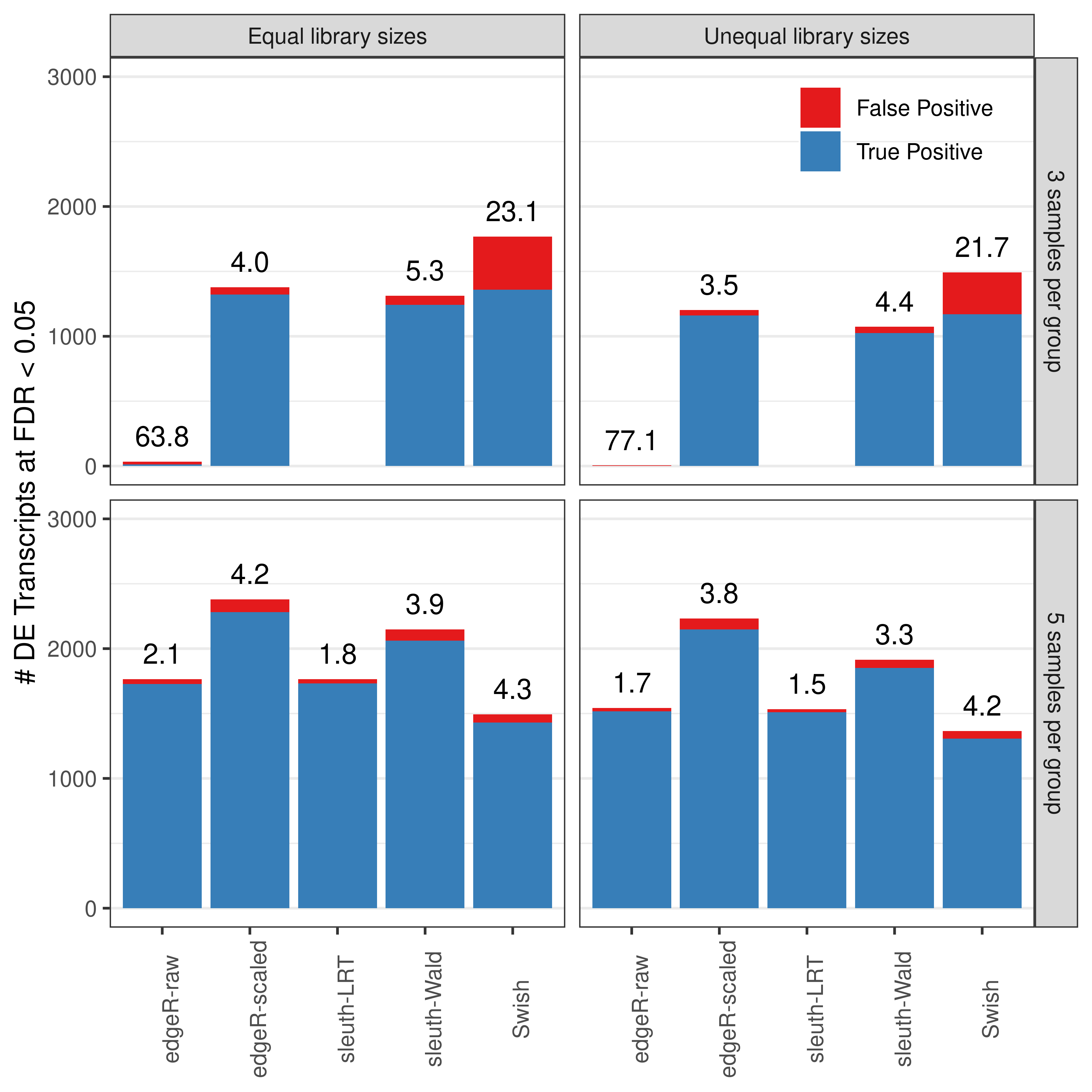
Average number of true (blue) and false (red) positive DE transcripts. Observed is FDR annotated over bars. Results from the simulation scenario with 100 bp paired-end read data quantified with Salmon, averaged over 20 simulations.
False discovery rate
dt.fdr.plot <- rbind(subsetDT(dt.fdr,scenario.balanced,'A'),
                     subsetDT(dt.fdr,scenario.unbalanced,'A'))

dt.fdr.plot$LibsPerGroup %<>%
  mapvalues(from = paste0('#Lib/Group = ', c(3, 5)),
            to = paste0(c(3,5),' samples per group'))

dt.fdr.plot$Scenario %<>%
  mapvalues(from = c('balanced','unbalanced'),
            to = c('Equal library sizes','Unequal library sizes'))

dt.fdr.plot <- dt.fdr.plot[TxPerGene == 'All Transcripts',]


plot <- ggplot(dt.fdr.plot,aes(x = N,y = FDR,color = Method,group = Method)) +
  facet_grid(rows = vars(LibsPerGroup),cols = vars(Scenario)) +
  geom_line(linewidth = 1) +
  theme_bw() +
  scale_color_manual(values = methodsNames()$color) +
  scale_y_continuous(limits = c(0,1250)) +
  theme(panel.grid = element_blank(),legend.direction = 'vertical',
        legend.position = c(0.125,0.88),legend.title = element_blank(),
        legend.background = element_rect(fill=alpha('white', 0))) +
  labs(y = 'False discoveries',x = 'Transcripts chosen')

plot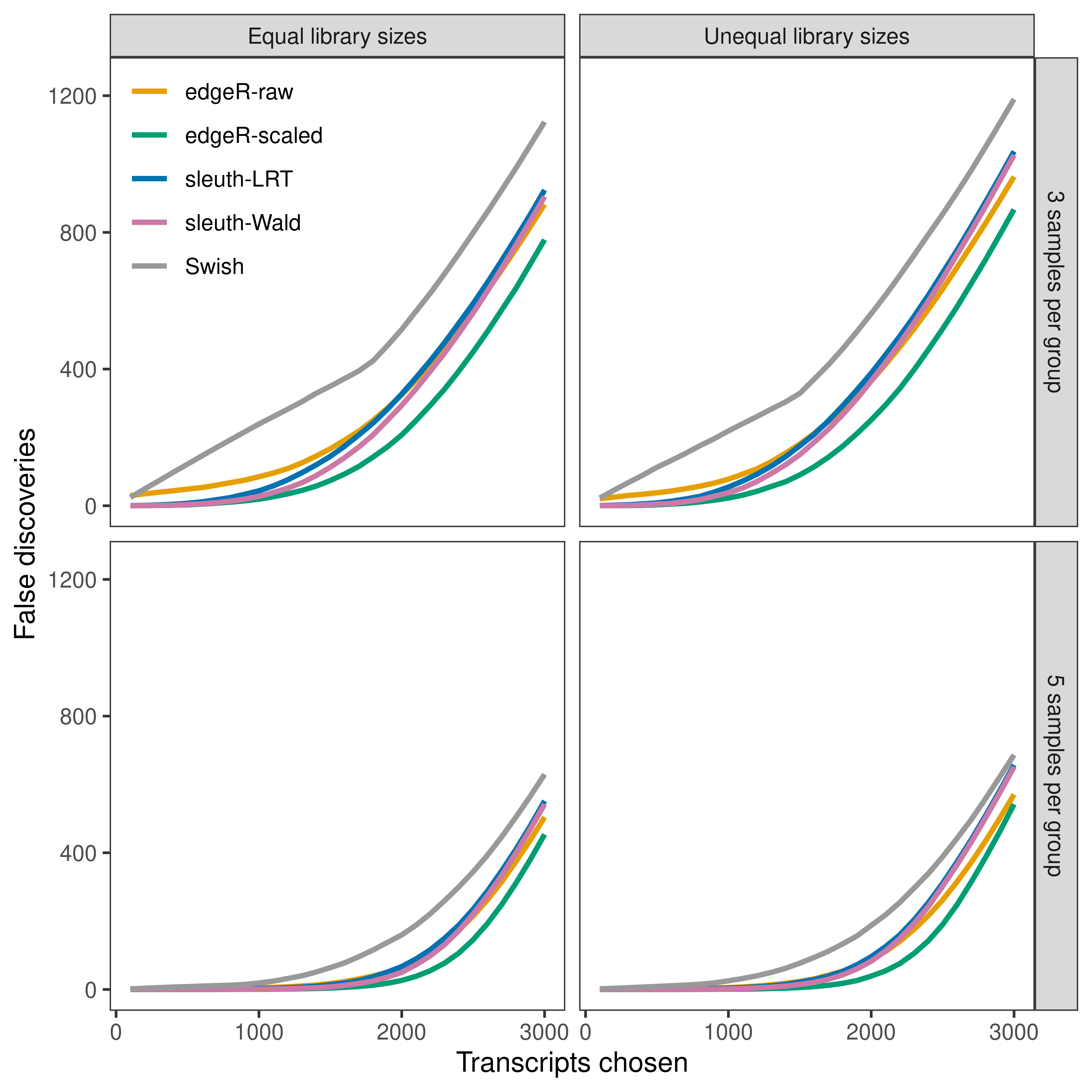
Average number of false discoveries as a function of the number of chosen transcripts. Results from the simulation scenario with 100 bp paired-end read data quantified with Salmon, averaged over 20 simulations.
Type 1 error
dt.type1error <- rbind(subsetDT(dt.metrics,scenario.balanced,'B'),
                       subsetDT(dt.metrics,scenario.unbalanced,'B'))

dt.type1error$LibsPerGroup %<>%
  mapvalues(from = paste0('#Lib/Group = ', c(3, 5)),
            to = paste0(c(3,5),' samples per group'))

dt.type1error$Scenario %<>%
  mapvalues(from = c('balanced','unbalanced'),
            to = c('Equal library sizes','Unequal library sizes'))

dt.type1error[, FDR := roundPretty(ifelse((FP+TP) == 0,NA,100*FP/(FP+TP)),1)]

dt.type1error <- dt.type1error[TxPerGene == 'All Transcripts',]


sub.byvar <-
  colnames(dt.type1error)[-which(colnames(dt.type1error) %in% c('P.SIG','TP','FP'))]

x.melt <-
  melt(dt.type1error,id.vars = sub.byvar,
       measure.vars = c('P.SIG'),variable.name = 'Type',value.name = 'Value')

plot <- ggplot(x.melt,aes(x = Method,y = Value)) +
  facet_grid(rows = vars(LibsPerGroup),cols = vars(Scenario)) +
  geom_col() +
  theme_bw() +
  geom_hline(yintercept = 0.05,color = 'red',linetype = 'dashed') +
  labs(x = NULL,y = paste('Proportion of transcripts with p-value < 0.05')) +
  theme(panel.grid.major.x = element_blank(),
        panel.grid.minor.x = element_blank(),
        panel.grid.minor.y = element_blank(),
        legend.position = 'top',legend.title = element_blank(),
        axis.text.x = element_text(angle = 90))

plot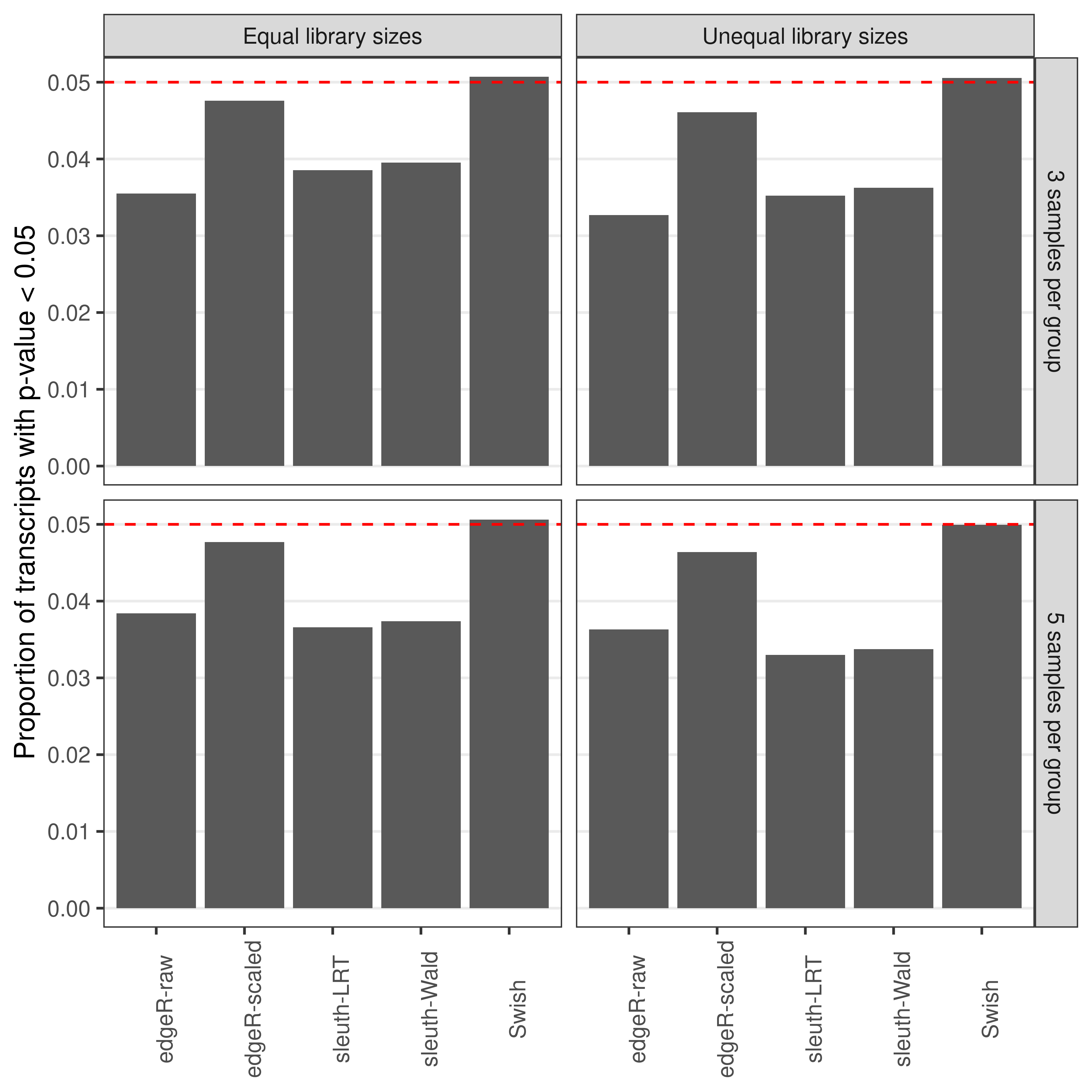
Average proportion of transcripts with unadjusted p-values less than 0.05. Results from the null simulation scenario with 100 bp paired-end read data quantified with Salmon, averaged over 20 simulations.
dt.pvalue.plot <- subsetDT(dt.pvalue,scenario.unbalanced,'C','All Transcripts')
dt.pvalue.plot <- dt.pvalue.plot[LibsPerGroup == '#Lib/Group = 5',]

plot <- ggplot(data = dt.pvalue.plot,aes(x = PValue,y = Density.Avg)) +
  facet_wrap('Method',nrow = 2) +
  geom_col(col = NA,fill = 'grey',position = position_dodge(),width = 0.75) +
  geom_smooth(aes(group = 1),se = FALSE,linewidth = 0.5,method = 'loess',span = 0.3) +
  geom_hline(yintercept = 1,col = 'red',linewidth = 0.5,linetype = 'dashed') +
  theme_bw() +
  theme(panel.grid = element_blank()) +
  scale_x_discrete(breaks = c("(0.00-0.05]","(0.50-0.55]","(0.95-1.00]"),
                   labels = c(0.00,0.50,1.00)) +
  labs(x = 'P-values',y = 'Density')

plot
`geom_smooth()` using formula = 'y ~ x'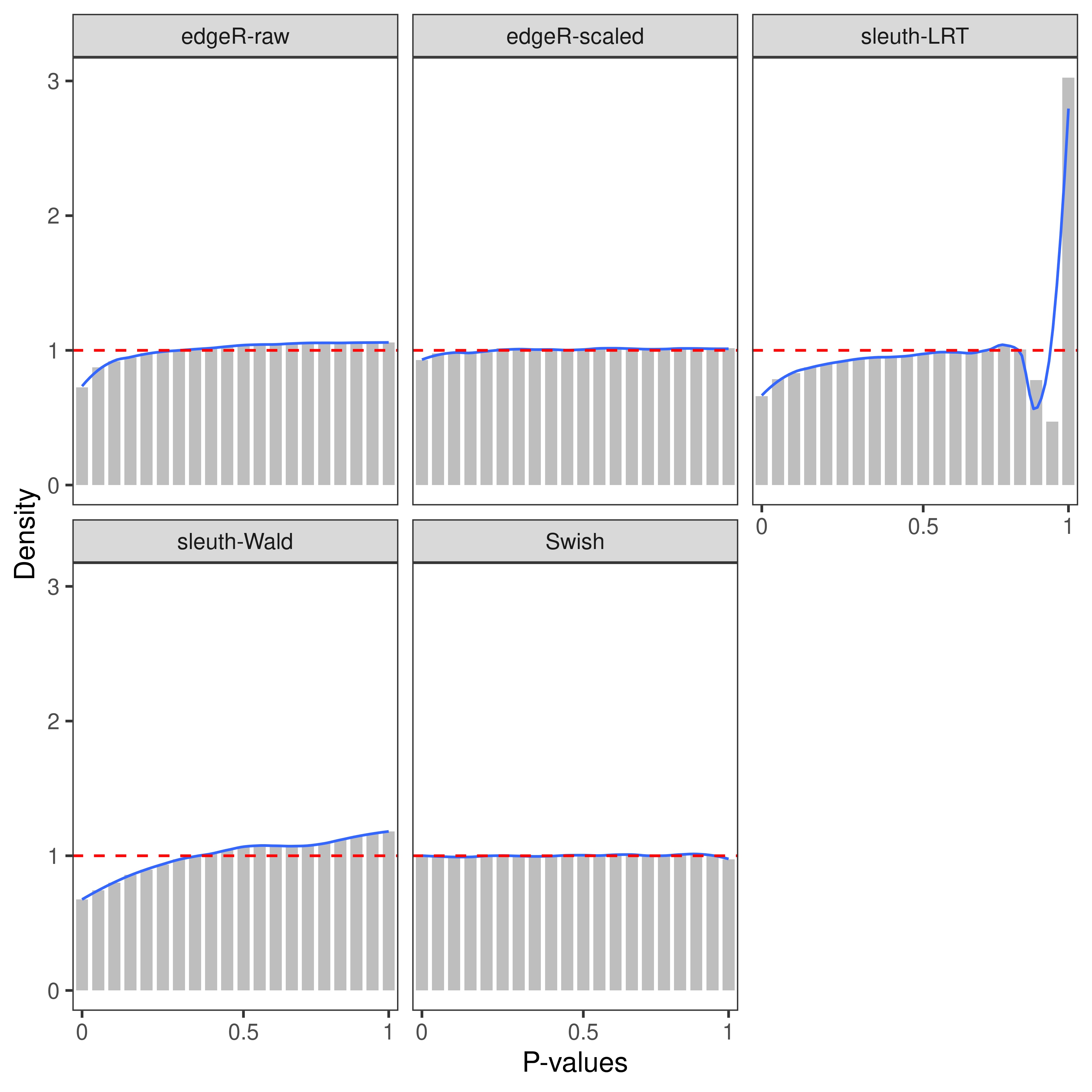
Density histograms with smoothing of raw p-values. Results from the null simulation scenario with 100 bp paired-end read data quantified with Salmon with 5 samples per group, averaged over 20 simulations.
sessionInfo()R version 4.2.1 (2022-06-23)
Platform: x86_64-pc-linux-gnu (64-bit)
Running under: CentOS Linux 7 (Core)
Matrix products: default
BLAS: /stornext/System/data/apps/R/R-4.2.1/lib64/R/lib/libRblas.so
LAPACK: /stornext/System/data/apps/R/R-4.2.1/lib64/R/lib/libRlapack.so
locale:
[1] LC_CTYPE=en_US.UTF-8 LC_NUMERIC=C
[3] LC_TIME=en_US.UTF-8 LC_COLLATE=en_US.UTF-8
[5] LC_MONETARY=en_US.UTF-8 LC_MESSAGES=en_US.UTF-8
[7] LC_PAPER=en_US.UTF-8 LC_NAME=C
[9] LC_ADDRESS=C LC_TELEPHONE=C
[11] LC_MEASUREMENT=en_US.UTF-8 LC_IDENTIFICATION=C
attached base packages:
[1] stats graphics grDevices utils datasets methods base
other attached packages:
[1] pkg_1.0 kableExtra_1.3.4 ggpubr_0.5.0
[4] readr_2.1.3 purrr_0.3.5 devtools_2.4.5
[7] usethis_2.1.6 BiocParallel_1.32.1 edgeR_3.40.0
[10] limma_3.54.0 magrittr_2.0.3 plyr_1.8.8
[13] thematic_0.1.2.1 ggplot2_3.4.0 data.table_1.14.6
[16] workflowr_1.7.0
loaded via a namespace (and not attached):
[1] utf8_1.2.2 tidyselect_1.2.0
[3] RSQLite_2.2.18 AnnotationDbi_1.60.0
[5] htmlwidgets_1.5.4 grid_4.2.1
[7] munsell_0.5.0 codetools_0.2-18
[9] miniUI_0.1.1.1 withr_2.5.0
[11] colorspace_2.0-3 Biobase_2.58.0
[13] filelock_1.0.2 highr_0.9
[15] knitr_1.41 rstudioapi_0.14
[17] stats4_4.2.1 SingleCellExperiment_1.20.0
[19] ggsignif_0.6.4 Rsubread_2.12.0
[21] labeling_0.4.2 MatrixGenerics_1.10.0
[23] git2r_0.30.1 tximport_1.26.0
[25] GenomeInfoDbData_1.2.9 bit64_4.0.5
[27] farver_2.1.1 rhdf5_2.42.0
[29] rprojroot_2.0.3 vctrs_0.5.1
[31] generics_0.1.3 xfun_0.35
[33] BiocFileCache_2.6.0 fishpond_2.4.0
[35] R6_2.5.1 GenomeInfoDb_1.34.3
[37] locfit_1.5-9.6 AnnotationFilter_1.22.0
[39] bitops_1.0-7 rhdf5filters_1.10.0
[41] cachem_1.0.6 DelayedArray_0.24.0
[43] assertthat_0.2.1 promises_1.2.0.1
[45] BiocIO_1.8.0 scales_1.2.1
[47] gtable_0.3.1 processx_3.8.0
[49] ensembldb_2.22.0 rlang_1.0.6
[51] systemfonts_1.0.4 splines_4.2.1
[53] rtracklayer_1.58.0 rstatix_0.7.1
[55] lazyeval_0.2.2 broom_1.0.1
[57] BiocManager_1.30.19 yaml_2.3.6
[59] abind_1.4-5 GenomicFeatures_1.50.2
[61] backports_1.4.1 httpuv_1.6.6
[63] sleuth_0.30.0 wasabi_1.0.1
[65] tools_4.2.1 ellipsis_0.3.2
[67] RColorBrewer_1.1-3 jquerylib_0.1.4
[69] BiocGenerics_0.44.0 sessioninfo_1.2.2
[71] Rcpp_1.0.9 progress_1.2.2
[73] zlibbioc_1.44.0 RCurl_1.98-1.9
[75] ps_1.7.2 prettyunits_1.1.1
[77] urlchecker_1.0.1 S4Vectors_0.36.0
[79] SummarizedExperiment_1.28.0 fs_1.5.2
[81] svMisc_1.2.3 whisker_0.4
[83] ProtGenerics_1.30.0 matrixStats_0.63.0
[85] pkgload_1.3.2 hms_1.1.2
[87] mime_0.12 evaluate_0.18
[89] xtable_1.8-4 XML_3.99-0.12
[91] IRanges_2.32.0 compiler_4.2.1
[93] biomaRt_2.54.0 tibble_3.1.8
[95] crayon_1.5.2 htmltools_0.5.3
[97] mgcv_1.8-41 later_1.3.0
[99] tzdb_0.3.0 tidyr_1.2.1
[101] DBI_1.1.3 dbplyr_2.2.1
[103] rappdirs_0.3.3 Matrix_1.5-3
[105] car_3.1-1 cli_3.4.1
[107] parallel_4.2.1 GenomicRanges_1.50.1
[109] pkgconfig_2.0.3 getPass_0.2-2
[111] GenomicAlignments_1.34.0 xml2_1.3.3
[113] svglite_2.1.0 bslib_0.4.1
[115] webshot_0.5.4 XVector_0.38.0
[117] rvest_1.0.3 stringr_1.4.1
[119] callr_3.7.3 digest_0.6.30
[121] Biostrings_2.66.0 rmarkdown_2.18
[123] tximeta_1.16.0 restfulr_0.0.15
[125] curl_4.3.3 shiny_1.7.3
[127] Rsamtools_2.14.0 gtools_3.9.3
[129] rjson_0.2.21 nlme_3.1-160
[131] lifecycle_1.0.3 jsonlite_1.8.3
[133] Rhdf5lib_1.20.0 carData_3.0-5
[135] desc_1.4.2 viridisLite_0.4.1
[137] fansi_1.0.3 pillar_1.8.1
[139] lattice_0.20-45 KEGGREST_1.38.0
[141] fastmap_1.1.0 httr_1.4.4
[143] pkgbuild_1.3.1 interactiveDisplayBase_1.36.0
[145] glue_1.6.2 remotes_2.4.2
[147] png_0.1-7 BiocVersion_3.16.0
[149] bit_4.0.5 stringi_1.7.8
[151] sass_0.4.3 profvis_0.3.7
[153] blob_1.2.3 AnnotationHub_3.6.0
[155] memoise_2.0.1 dplyr_1.0.10