R Notebook
Last updated: 2019-12-02
Checks: 6 0
Knit directory: 10x-adipocyte-analysis/
This reproducible R Markdown analysis was created with workflowr (version 1.2.0). The Report tab describes the reproducibility checks that were applied when the results were created. The Past versions tab lists the development history.
Great! Since the R Markdown file has been committed to the Git repository, you know the exact version of the code that produced these results.
Great job! The global environment was empty. Objects defined in the global environment can affect the analysis in your R Markdown file in unknown ways. For reproduciblity it’s best to always run the code in an empty environment.
The command set.seed(20181026) was run prior to running the code in the R Markdown file. Setting a seed ensures that any results that rely on randomness, e.g. subsampling or permutations, are reproducible.
Great job! Recording the operating system, R version, and package versions is critical for reproducibility.
Nice! There were no cached chunks for this analysis, so you can be confident that you successfully produced the results during this run.
Great! You are using Git for version control. Tracking code development and connecting the code version to the results is critical for reproducibility. The version displayed above was the version of the Git repository at the time these results were generated.
Note that you need to be careful to ensure that all relevant files for the analysis have been committed to Git prior to generating the results (you can use wflow_publish or wflow_git_commit). workflowr only checks the R Markdown file, but you know if there are other scripts or data files that it depends on. Below is the status of the Git repository when the results were generated:
Ignored files:
    Ignored:    code/.Rhistory
    Ignored:    figures/
    Ignored:    output/bulk_analysis/
    Ignored:    output/demuxlet/
    Ignored:    output/harmony/
    Ignored:    output/markergenes/
    Ignored:    output/monocle/
    Ignored:    output/seurat_objects/
    Ignored:    output/velocyto/
    Ignored:    output/wgcna/
    Ignored:    tables/

Untracked files:
    Untracked:  .rstudio_old10/
    Untracked:  10x-adipocyte-analysis-copy.Rproj
    Untracked:  analysis/.ipynb_checkpoints/10x-180831_harmony_palantir-checkpoint.ipynb
    Untracked:  analysis/.ipynb_checkpoints/velocyto_notebook_180831-checkpoint.ipynb
    Untracked:  code/BEAM-heatmaps.R
    Untracked:  code/BEAM_gsea.R
    Untracked:  code/__pycache__/
    Untracked:  code/colors.R
    Untracked:  code/convert_raw_data_to_csv_harmony.R
    Untracked:  code/harmony.py
    Untracked:  code/test.csv

Unstaged changes:
    Deleted:    10x-adipocyte-analysis.Rproj
    Deleted:    analysis/velocyto_notebook_180504.ipynb
    Deleted:    analysis/velocyto_notebook_180831.ipynb
    Modified:   analysis/wolfrum-scmap.Rmd
    Deleted:    code/REMOVE/find-brown-sample-markers-180504-REMOVE.R
    Deleted:    code/REMOVE/find-white-sample-markers-180504-REMOVE.R
    Deleted:    code/REMOVE/get-genes-monocle-180831-REMOVE.R
    Modified:   code/compute-genelists-monocle-depots.R
    Modified:   code/find-depot-markers-180504.R
    Modified:   code/find-markers.R
    Modified:   code/preprocess-data.R
    Modified:   code/run-alignment.R
    Modified:   code/run-monocle.R
    Modified:   code/velocyto_preprocess.py
Note that any generated files, e.g. HTML, png, CSS, etc., are not included in this status report because it is ok for generated content to have uncommitted changes.
These are the previous versions of the R Markdown and HTML files. If you’ve configured a remote Git repository (see ?wflow_git_remote), click on the hyperlinks in the table below to view them.
| File | Version | Author | Date | Message |
|---|---|---|---|---|
| Rmd | 6e9bd41 | Pytrik Folkertsma | 2019-12-02 | wflow_publish(c(“analysis/wolfrum_analysis.Rmd”)) |
| html | bdb871b | Pytrik Folkertsma | 2019-12-02 | Build site. |
| Rmd | a3dbe85 | Pytrik Folkertsma | 2019-12-02 | wflow_publish(c(“analysis/wolfrum_analysis.Rmd”)) |
| html | d28b5ef | Pytrik Folkertsma | 2019-11-15 | Build site. |
| Rmd | 55cb46e | Pytrik Folkertsma | 2019-11-15 | wolfrum analysis |
| Rmd | 5cffa21 | Pytrik Folkertsma | 2019-11-13 | wolfrum analysis |
| Rmd | 9ae091e | Pytrik Folkertsma | 2019-11-12 | wolfrum branch markers |
library(Seurat)
library(monocle)
library(cowplot)
library(dplyr)
library(tidyr)
library(knitr)
library(kableExtra)
library(DT)
wolfrum <- readRDS('/projects/timshel/sc-scheele_lab_adipose_fluidigm_c1/data-wolfrum/wolfrum.compute.seurat_obj.rds')
data_180831 <- readRDS('/projects/pytrik/sc_adipose/analyze_10x_fluidigm/10x-adipocyte-analysis/output/seurat_objects/180831/10x-180831-S3')Which clusters are adipocytes/preadipocytes?
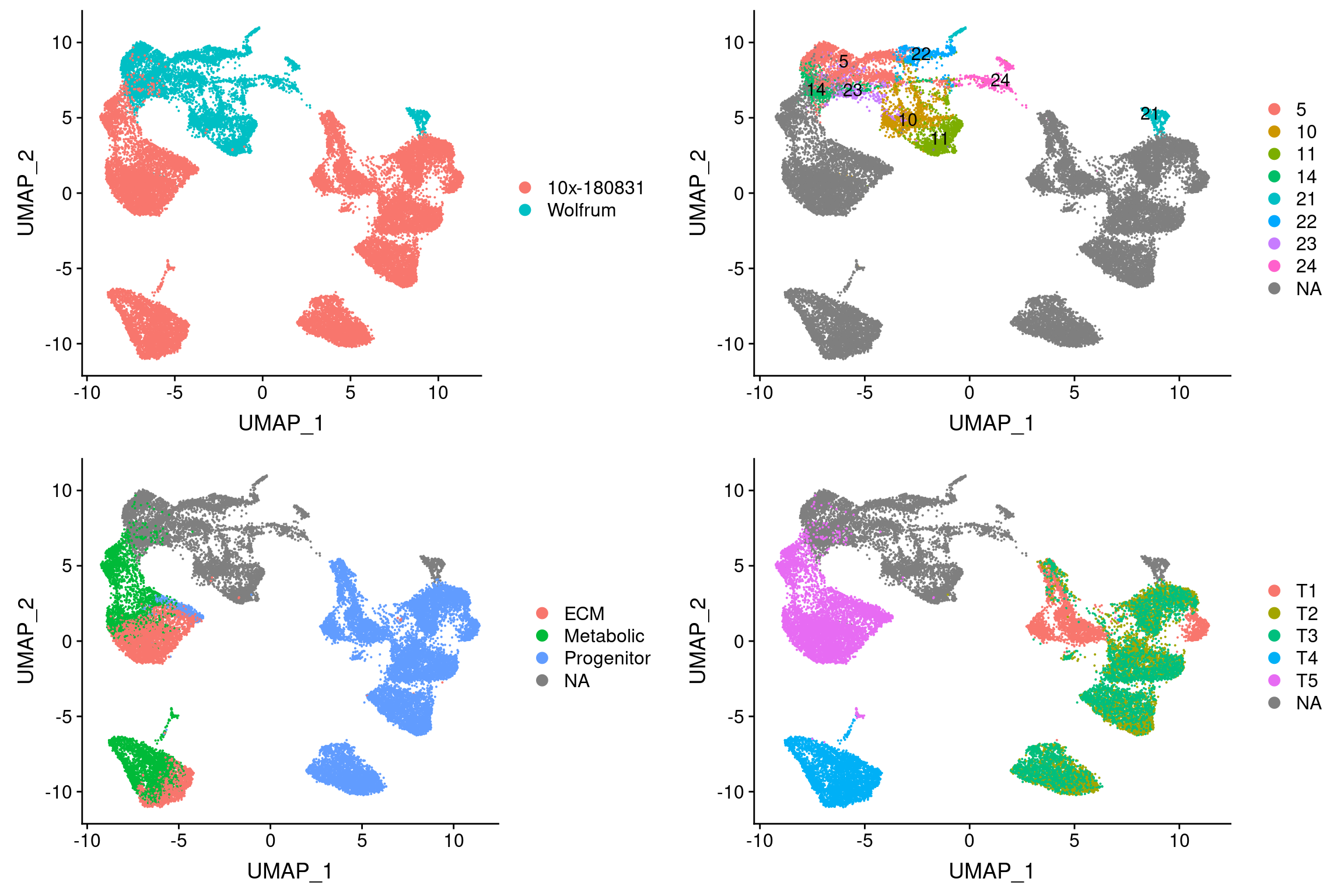
plot_grid(
  UMAPPlot(wolfrum, group.by='orig.ident', label=T),
  UMAPPlot(wolfrum, group.by='seurat_clusters', label=T)
)
| Version | Author | Date |
|---|---|---|
| d28b5ef | Pytrik Folkertsma | 2019-11-15 |
markers <- read.table('output/markergenes/wolfrum/markers_wolfrum.compute.seurat_obj.rds_seurat_clusters_negbinom', sep='\t', header=T)Top 10 positive markers per cluster
pos_markers_top10 <- markers %>%
  group_by(cluster) %>%
  top_n(n=10, wt=avg_logFC)

neg_markers_top20 <- markers %>%
  group_by(cluster) %>%
  top_n(n=6, wt=desc(avg_logFC))

pos_markers_top10
# A tibble: 270 x 7
# Groups: cluster [27]
cluster p_val avg_logFC pct.1 pct.2 p_val_adj gene
<int> <dbl> <dbl> <dbl> <dbl> <dbl> <fct>
1 0 0 -0.250 0.04 0.213 0 NHLRC2
2 0 0 -0.250 0.046 0.242 0 KANSL3
3 0 0 -0.250 0.041 0.238 0 PSMA5
4 0 0 -0.250 0.077 0.248 0 ZNF106
5 0 0 -0.250 0.045 0.201 0 C9orf85
6 0 0 -0.250 0.042 0.247 0 ILKAP
7 0 0 -0.250 0.037 0.24 0 PHF11
8 0 0 -0.250 0.05 0.242 0 SEL1L
9 0 0 -0.251 0.044 0.255 0 KLC1
10 0 0 -0.251 0.034 0.192 0 DZIP3
# … with 260 more rowsWhich clusters are the preadipocytes? Check by plotting some of the DE genes between T1T2T3 and T4T5 in the 180831 dataset.
#DE genes between T1T2T3 and T4T5 in the 10x-180831 data.
markers_T1T2T3_T4T5 <- read.table('output/markergenes/180831/markers_10x-180831_time_combined_negbinom', header=T)
markers_T1T2T3_T4T5 <- markers_T1T2T3_T4T5[order(-markers_T1T2T3_T4T5$avg_logFC),]
markers_T1T2T3 <- markers_T1T2T3_T4T5[which(markers_T1T2T3_T4T5$cluster == 1),]
markers_T4T5 <- markers_T1T2T3_T4T5[which(markers_T1T2T3_T4T5$cluster == 2),]
How do these genes look in the 180831 data?
plots <- FeaturePlot(data_180831, features=c(as.vector(markers_T1T2T3$gene)[1:10], as.vector(markers_T4T5$gene)[1:10]), pt.size=1, combine=F)
plot_grid(plotlist=plots, ncol=4)
| Version | Author | Date |
|---|---|---|
| d28b5ef | Pytrik Folkertsma | 2019-11-15 |
How are they expressed in the Wolfrum data?
plots <- FeaturePlot(wolfrum, features=c(as.vector(markers_T1T2T3$gene)[1:10], as.vector(markers_T4T5$gene)[1:10]), pt.size=1, combine=F)
plot_grid(plotlist=plots, ncol=2)
| Version | Author | Date |
|---|---|---|
| d28b5ef | Pytrik Folkertsma | 2019-11-15 |
Not all genes are expressed clearly in specific clusters. It looks like cluster 22, 21, 5, 14, 23, 11 and 10 are the preadipocytes.
UMAPPlot(wolfrum, group.by='seurat_clusters', label=T)
| Version | Author | Date |
|---|---|---|
| d28b5ef | Pytrik Folkertsma | 2019-11-15 |
Also plot the top 10 ECM and Metabolic markers.
#DE genes between T1T2T3 and T4T5 in the 10x-180831 data.
markers_u_l <- read.table('output/markergenes/180831/markers_10x-180831_upperbranch_lowerbranch_negbinom', sep='\t', header=T)
markers_u <- markers_u_l[order(-markers_u_l$avg_logFC),]
markers_l <- markers_u_l[order(markers_u_l$avg_logFC),]
How do these genes look in the 180831 data?
plots <- FeaturePlot(data_180831, features=c(as.vector(markers_u$gene)[1:10], as.vector(markers_l$gene)[1:10]), pt.size=1, combine=F)
plot_grid(plotlist=plots, ncol=4)
| Version | Author | Date |
|---|---|---|
| d28b5ef | Pytrik Folkertsma | 2019-11-15 |
And how are they expressed in the Wolfrum data?
plots <- FeaturePlot(wolfrum, features=c(as.vector(markers_u$gene)[1:10], as.vector(markers_l$gene)[1:10]), pt.size=1, combine=F)Warning in FetchData(object = object, vars = c(dims, "ident", features), :
The following requested variables were not found: RP11-572C15.6plot_grid(plotlist=plots, ncol=2)
| Version | Author | Date |
|---|---|---|
| d28b5ef | Pytrik Folkertsma | 2019-11-15 |
The U and L branch markers are clearly expressed in the two clusters in the top right of the UMAP plot.
Check how many of the marker genes are found in each cluster.
get_gene_overlap_per_cluster <- function(min_logFC, n_genes){
  pos_markers <- markers[markers$avg_logFC > min_logFC,]

  genes_P <- c(as.vector(markers_T1T2T3$gene)[1:n_genes])
  #genes_P <- c(as.vector(markers_T1T2T3$gene)[1:n_genes], as.vector(markers_T4T5$gene)[1:n_genes])
  genes_U <- as.vector(markers_u$gene)[1:n_genes]
  genes_L <- as.vector(markers_l$gene)[1:n_genes]
  all_genes <- unique(c(genes_P, genes_U, genes_L))

  df <- as.data.frame(matrix(ncol=4, nrow=length(unique(pos_markers$cluster))))
  colnames(df) <- c('total_overlap', 'overlap_P', 'overlap_L', 'overlap_U')
  rownames(df) <- unique(pos_markers$cluster)

  for (i in 1:length(unique(pos_markers$cluster))){
    genes_cluster <- as.vector(pos_markers[pos_markers$cluster == i,]$gene)
    df[i, 'overlap_P'] <- round(length(intersect(genes_cluster, genes_P)) / length(genes_P), 2)
    df[i, 'overlap_L'] <- round(length(intersect(genes_cluster, genes_L)) / length(genes_L), 2)
    df[i, 'overlap_U'] <- round(length(intersect(genes_cluster, genes_U)) / length(genes_U), 2)
    df[i, 'total_overlap'] <- round(length(intersect(genes_cluster, all_genes)) / length(all_genes), 2)
  }
  return(df)
}

print_top_clusters <- function(df){
  print(paste('P: ', toString(rownames(df[order(-df$overlap_P),][1:3,])), sep=''))
  print(paste('L: ', toString(rownames(df[order(-df$overlap_L),][1:3,])), sep=''))
  print(paste('U: ', toString(rownames(df[order(-df$overlap_U),][1:3,])), sep=''))
}
Table shows the percentage of genes with avgLogFC > 0.7 that was found in the cluster. Sort on columns to get the top clusters.
logfc_0.5_genes_100 <- get_gene_overlap_per_cluster(0.5, 100)
datatable(logfc_0.5_genes_100)
Check the top 5 clusters per branch for different n_genes and min logFC
logfc <- c(0.25, 0.5, 0.7)
n_genes <- c(100, 100, 100)
for (i in 1:length(logfc)){
  print(paste('min_logFC: ', logfc[i], ' | n_genes: ', n_genes[i], sep=''))
  df <- get_gene_overlap_per_cluster(logfc[i], n_genes[i])
  print_top_clusters(df)
}
[1] "min_logFC: 0.25 | n_genes: 100"
[1] "P: 24, 11, 22"
[1] "L: 11, 10, 23"
[1] "U: 14, 24, 23"
[1] "min_logFC: 0.5 | n_genes: 100"
[1] "P: 24, 11, 22"
[1] "L: 11, 10, 23"
[1] "U: 14, 23, 24"
[1] "min_logFC: 0.7 | n_genes: 100"
[1] "P: 24, 11, 19"
[1] "L: 11, 10, 23"
[1] "U: 14, 23, 22"There is some overlap between branches which is good. Cluster 11 is shared between P and L, cluster 14 is shared between P and U and cluster 23 is shared between L and U. This would indicate that cluster 24 contains most immature preadipocytes, cluster 10 contains most mature L branch cells and cluster 22 contains most mature U branch cells.\
Based on the results:\ P = 24\ L = 11\ U = 14\
Hypothesis: cluster 23 represents preadipocytes at the start of differentation (the cell states between T3 and T4 in 180831 data that we missed). Cluster 5 represents even more mature metabolic cells and cluster 11 represents more mature ECM cells.\
Clusters 22 shares most genes with the P branch. Cluster 23 most with the U branch. (see datatable above). These could also represent the preadipocytes at start of differentiation or the cells that transfer back to progenitor cells. \
UMAPPlot(wolfrum, group.by='seurat_clusters', label=T)
| Version | Author | Date |
|---|---|---|
| d28b5ef | Pytrik Folkertsma | 2019-11-15 |
#Idents(wolfrum) <- wolfrum@meta.data$seurat_clusters
#preadipocyte_subset <- subset(wolfrum, idents=c(5, 14, 23, 11, 10, 21, 22, 24))
#preadipocyte_subset <- FindVariableFeatures(preadipocyte_subset)
#preadipocyte_subset <- ScaleData(preadipocyte_subset)
#preadipocyte_subset <- RunPCA(object=preadipocyte_subset, npcs=30)
#ElbowPlot(preadipocyte_subset, ndims=30)
#preadipocyte_subset <- FindNeighbors(object = preadipocyte_subset, dims=1:13)
#preadipocyte_subset <- FindClusters(object = preadipocyte_subset, resolution=0.8)
#preadipocyte_subset <- RunTSNE(object = preadipocyte_subset, dims=1:13)
#preadipocyte_subset <- RunUMAP(object = preadipocyte_subset, dims=1:13)
#saveRDS(preadipocyte_subset, '/projects/pytrik/sc_adipose/analyze_10x_fluidigm/10x-adipocyte-analysis/output/seurat_objects/wolfrum/wolfrum.preadipocyte_subset.rds')
preadipocyte_subset <- readRDS('output/seurat_objects/wolfrum/wolfrum.preadipocyte_subset.rds')

plot_grid(
  UMAPPlot(preadipocyte_subset, group.by='all_data_seurat_clusters', label=T),
  TSNEPlot(preadipocyte_subset, group.by='all_data_seurat_clusters', label=T)
)
| Version | Author | Date |
|---|---|---|
| d28b5ef | Pytrik Folkertsma | 2019-11-15 |
Seurat integration of Wolfrum and 10x-180831 data
#anchors <- FindIntegrationAnchors(object.list = list(wolfrum, data_180831), dims = 1:20)
#integrated <- IntegrateData(anchorset = anchors, dims = 1:20)
#saveRDS(integrated, '/projects/pytrik/sc_adipose/analyze_10x_fluidigm/10x-adipocyte-analysis/output/seurat_objects/wolfrum/wolfrum.180831.integrated.rds')
integrated <- readRDS('output/seurat_objects/wolfrum/wolfrum.180831.integrated.rds')
integrated@meta.data['dataset'] <- '10x-180831'
integrated@meta.data[which(is.na(integrated@meta.data$branch)), 'dataset'] <- 'Wolfrum'

plot_grid(
  UMAPPlot(integrated, group.by='dataset'),
  UMAPPlot(integrated, group.by='seurat_clusters', label=T),
  UMAPPlot(integrated, group.by='branch'), ncol=2
)
| Version | Author | Date |
|---|---|---|
| d28b5ef | Pytrik Folkertsma | 2019-11-15 |
These results also confirm that the L branch is closest to cluster 11 and U is closest to the U branch.\
Seurat integration of Wolfrum preadiopcyte subset and 10x-180831 data
integrated.subset <- readRDS('output/seurat_objects/wolfrum/wolfrum.preadipocyte_subset.180831.integrated.rds')

integrated.subset@meta.data['dataset'] <- '10x-180831'
integrated.subset@meta.data[which(is.na(integrated.subset@meta.data$branch)), 'dataset'] <- 'Wolfrum'
integrated.subset <- AddMetaData(integrated.subset, metadata=wolfrum@meta.data['seurat_clusters'])

plot_grid(
  UMAPPlot(integrated.subset, group.by='dataset'),
  UMAPPlot(integrated.subset, group.by='seurat_clusters', label=T),
  UMAPPlot(integrated.subset, group.by='branch'),
  UMAPPlot(integrated.subset, group.by='timepoint'), ncol=2
)
| Version | Author | Date |
|---|---|---|
| d28b5ef | Pytrik Folkertsma | 2019-11-15 |
Predict cell types with Seurat’s TransferData
wolfrum.predicted_labels <- readRDS('output/seurat_objects/wolfrum/wolfrum.predicted_labels_180831.rds')Used pca, pca.project and cca as dimred for FindTransferAnchors and IntegrateData. \
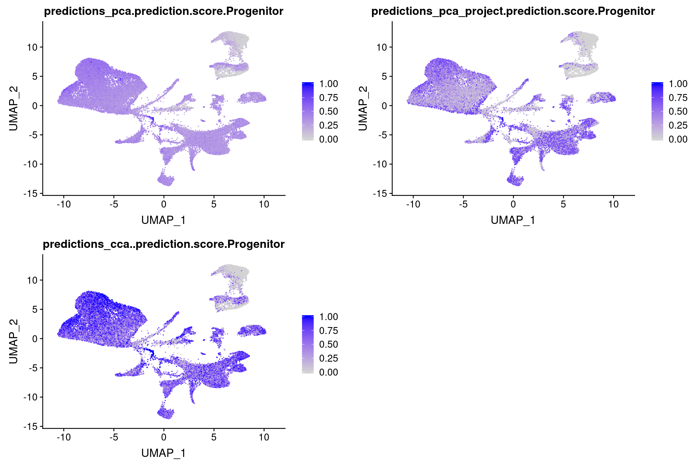
Scores for P cells
plot_grid(
  FeaturePlot(wolfrum.predicted_labels, features='predictions_pca.prediction.score.Progenitor'),
  FeaturePlot(wolfrum.predicted_labels, features='predictions_pca_project.prediction.score.Progenitor'),
  FeaturePlot(wolfrum.predicted_labels, features='predictions_cca..prediction.score.Progenitor'), ncol=2
)
| Version | Author | Date |
|---|---|---|
| d28b5ef | Pytrik Folkertsma | 2019-11-15 |
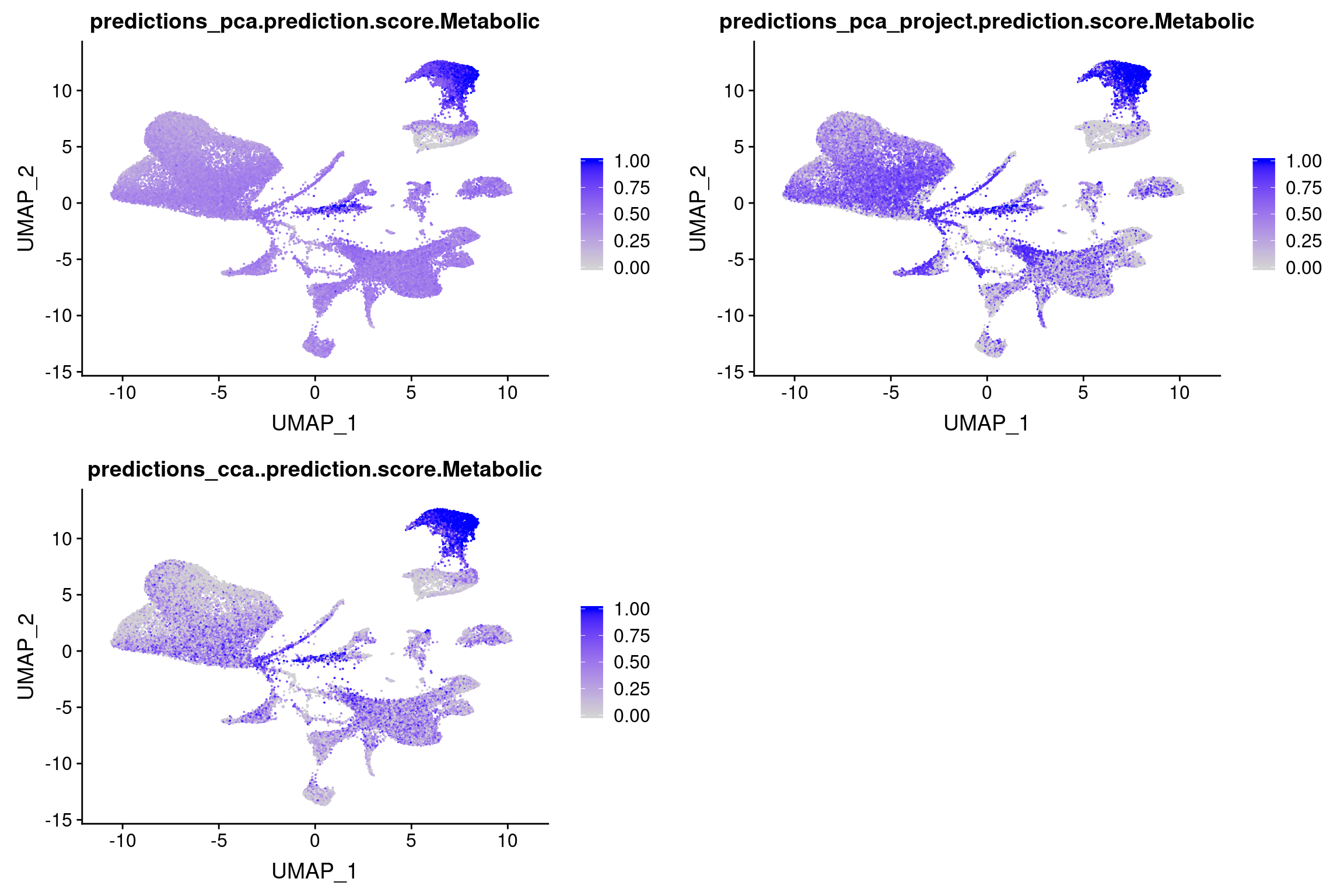
Scores for U cells
plot_grid(
  FeaturePlot(wolfrum.predicted_labels, features='predictions_pca.prediction.score.Metabolic'),
  FeaturePlot(wolfrum.predicted_labels, features='predictions_pca_project.prediction.score.Metabolic'),
  FeaturePlot(wolfrum.predicted_labels, features='predictions_cca..prediction.score.Metabolic'), ncol=2
)
| Version | Author | Date |
|---|---|---|
| d28b5ef | Pytrik Folkertsma | 2019-11-15 |
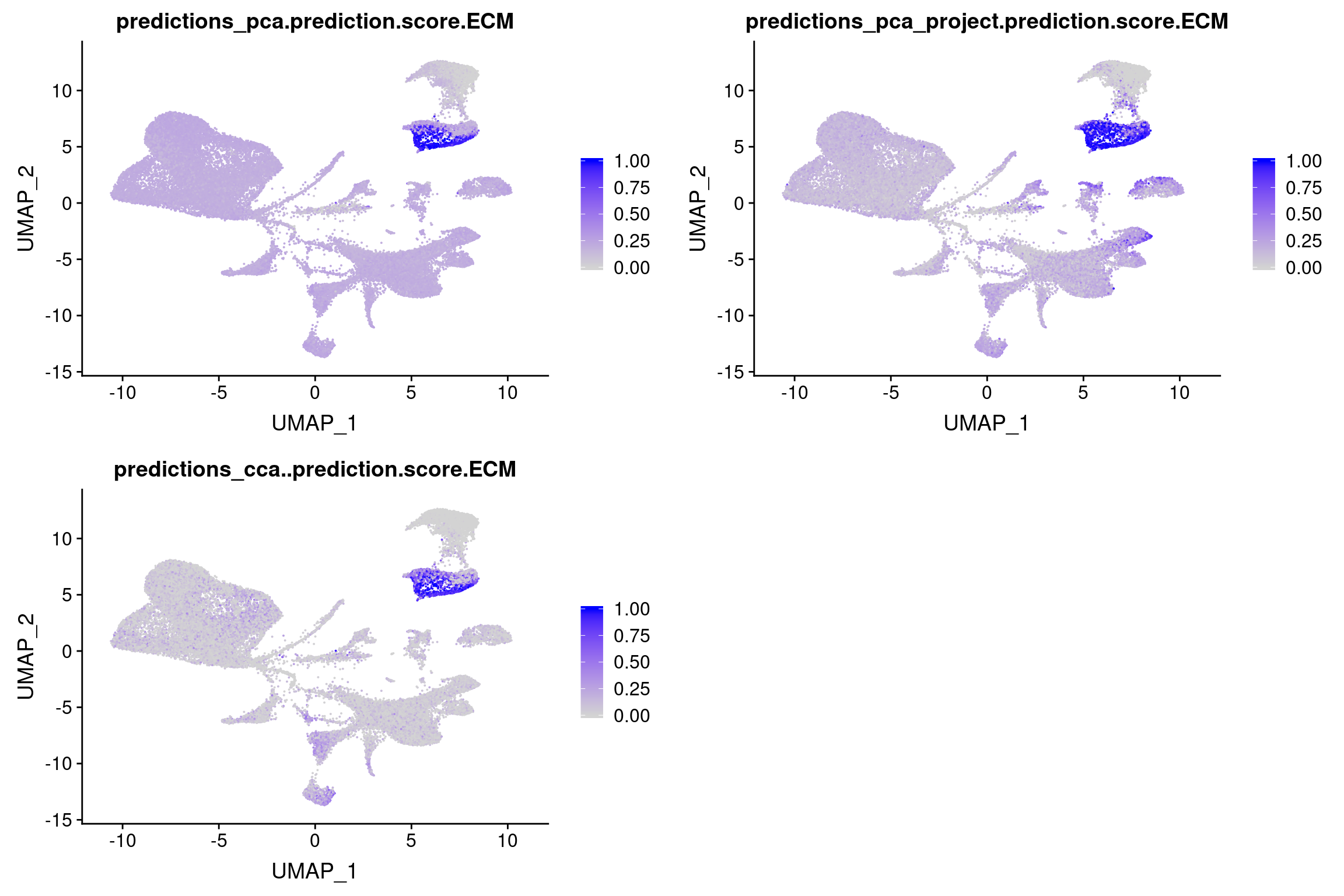
Scores for L cells
plot_grid(
  FeaturePlot(wolfrum.predicted_labels, features='predictions_pca.prediction.score.ECM'),
  FeaturePlot(wolfrum.predicted_labels, features='predictions_pca_project.prediction.score.ECM'),
  FeaturePlot(wolfrum.predicted_labels, features='predictions_cca..prediction.score.ECM'), ncol=2
)
| Version | Author | Date |
|---|---|---|
| d28b5ef | Pytrik Folkertsma | 2019-11-15 |
For all predictions, change predicted id to NA if max score is below a certain threshold.
assign_labels <- function(colname, threshold=0.5){
pred_ids <- unlist(as.vector(apply(wolfrum.predicted_labels@meta.data[,c(paste(colname,'.prediction.score.max', sep=''), paste(colname, '.predicted.id', sep=''))], 1, function(x){
if (x[[1]] < threshold){
return(NA)
} else{
return(x[[2]])
}
})))
return(pred_ids)
}
for (col in c('predictions_pca_project', 'predictions_pca', 'predictions_cca.')){
for (t in c(0.5, 0.7, 0.9, 0.95, 0.99)){
preds <- assign_labels(col, t)
wolfrum.predicted_labels <- AddMetaData(wolfrum.predicted_labels, preds, col.name=paste(col, 'predicted_label', t, sep='.'))
}
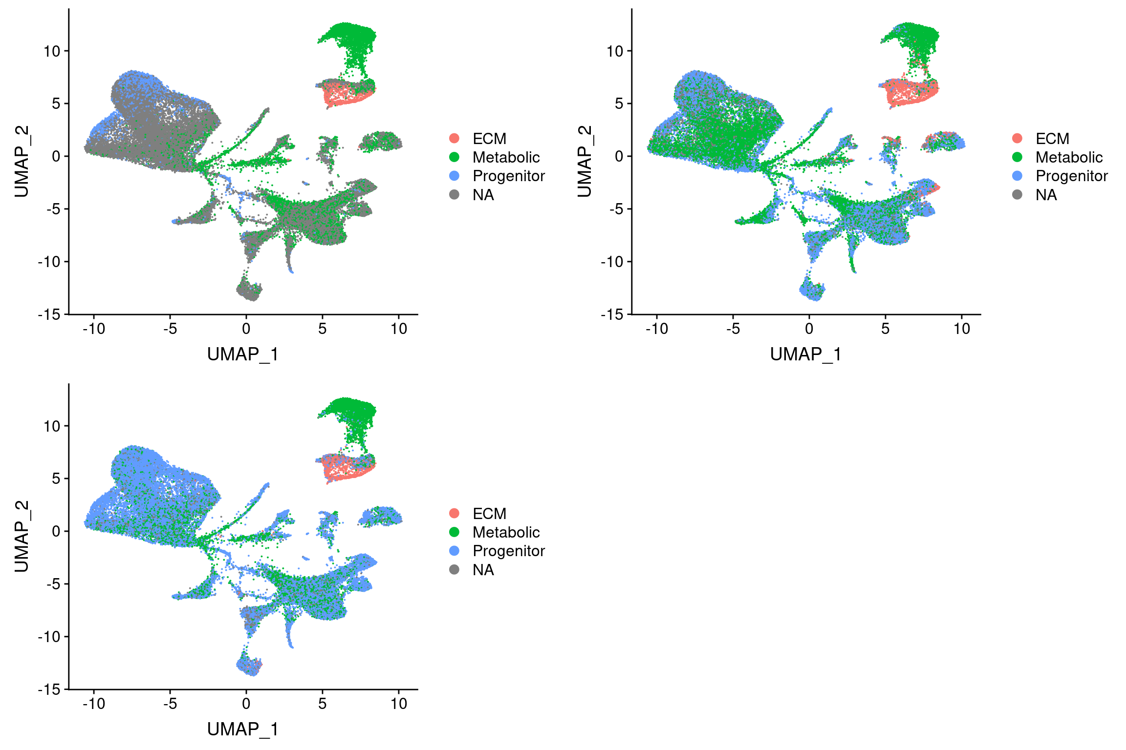
}Threshold for prediction = 0.5
plot_grid(
  UMAPPlot(wolfrum.predicted_labels, group.by='predictions_pca.predicted_label.0.5'),
  UMAPPlot(wolfrum.predicted_labels, group.by='predictions_pca_project.predicted_label.0.5'),
  UMAPPlot(wolfrum.predicted_labels, group.by='predictions_cca..predicted_label.0.5'), ncol=2
)
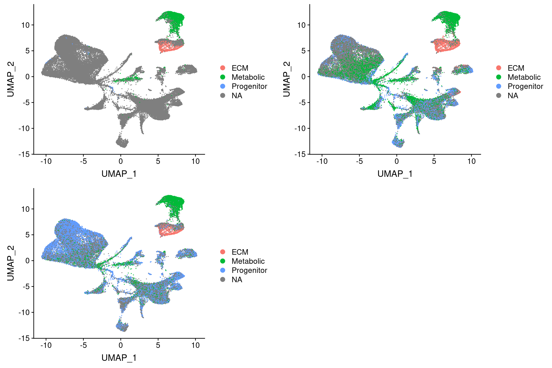
Threshold for prediction = 0.7
plot_grid(
  UMAPPlot(wolfrum.predicted_labels, group.by='predictions_pca.predicted_label.0.7'),
  UMAPPlot(wolfrum.predicted_labels, group.by='predictions_pca_project.predicted_label.0.7'),
  UMAPPlot(wolfrum.predicted_labels, group.by='predictions_cca..predicted_label.0.7'), ncol=2
)
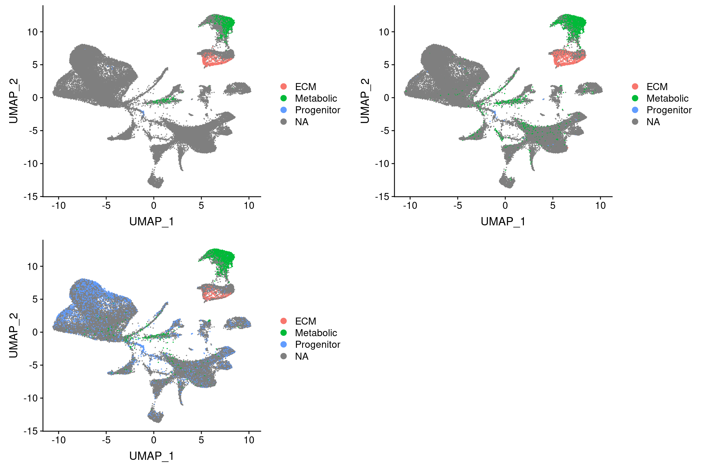
Threshold for prediction = 0.9
plot_grid(
  UMAPPlot(wolfrum.predicted_labels, group.by='predictions_pca.predicted_label.0.9'),
  UMAPPlot(wolfrum.predicted_labels, group.by='predictions_pca_project.predicted_label.0.9'),
  UMAPPlot(wolfrum.predicted_labels, group.by='predictions_cca..predicted_label.0.9'), ncol=2
)
| Version | Author | Date |
|---|---|---|
| bdb871b | Pytrik Folkertsma | 2019-12-02 |
Only show preadipocytes
clusters <- c(24, 22, 11, 10, 23, 5, 14)

adipocytes <- unlist(lapply(wolfrum.predicted_labels@meta.data$RNA_snn_res.0.8, function(x){
  if (x %in% clusters){
    return('preadipocyte')
  } else {
    return('non-preadipocyte')
  }
}))

wolfrum.predicted_labels@meta.data['preadipocytes'] <- adipocytes

for (col in c('predictions_pca_project', 'predictions_pca', 'predictions_cca.')){
  for (t in c(0.5, 0.7, 0.9, 0.95, 0.99)){
    preds <- assign_labels(col, t)
    wolfrum.predicted_labels <- AddMetaData(wolfrum.predicted_labels, preds, col.name=paste(col, 'predicted_label', t, sep='.'))
  }
}
Figures
labels <- unlist(lapply(wolfrum.predicted_labels@meta.data$predictions_pca.predicted_label.0.7, function(x){
  if (is.na(x)){
    return('Non-matching cells')
  } else if(x == 'ECM'){
    return('L')
  } else if(x == 'Metabolic'){
    return('U')
  } else if (x == 'Progenitor'){
    return('P')
  }
}))

wolfrum.predicted_labels@meta.data['predictions_pca.predicted_label.0.7_labels'] <- labels

wolfrum.predicted_labels@meta.data['predictions_pca.predicted_label.0.7_labels'] <- factor(wolfrum.predicted_labels@meta.data$predictions_pca.predicted_label.0.7_labels, levels = c("P", "L", "U", 'Non-matching cells'))
colormap.branches <- c(
P="#ecdd83",
U="#e27268",
L="#93c8bc",
'Non-matching cells'='#7a7a7a')
p_predictions <- UMAPPlot(wolfrum.predicted_labels, group.by='predictions_pca.predicted_label.0.7_labels', cols=colormap.branches, no.axes=T) + theme(legend.text=element_text(size=12), legend.key.height=unit(0.4, 'cm'), axis.text = element_blank(), axis.ticks = element_blank(), axis.title = element_blank(), plot.margin=grid::unit(c(0,0,0,0), "mm")) + labs(color='Seurat prediction') The following functions and any applicable methods accept the dots: CombinePlotsp_predictions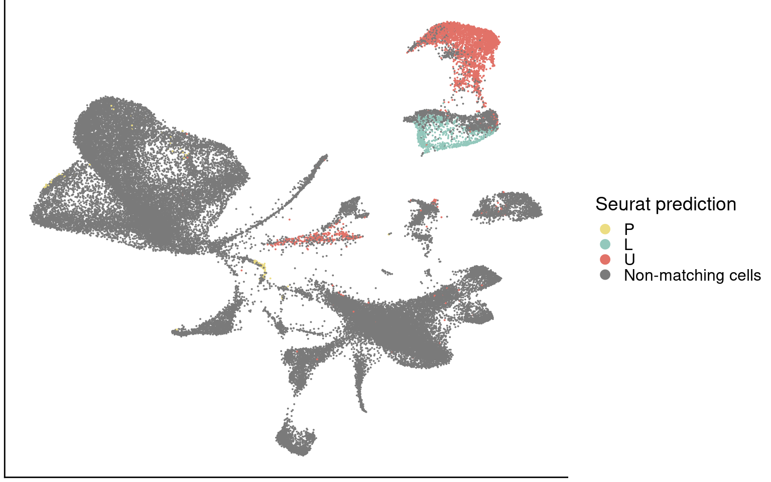
| Version | Author | Date |
|---|---|---|
| bdb871b | Pytrik Folkertsma | 2019-12-02 |
#save_plot("figures/figures_paper/main_figures/Figure_wolfrum/UMAP_wolfrum_predicted-labels_180831.pdf", p_predictions, base_width=8, base_height=5)p_clusters <- UMAPPlot(wolfrum.predicted_labels, group.by='RNA_snn_res.0.8', label=T, no.axes=T, no.legend=T) + theme(legend.position = "none", axis.text = element_blank(), axis.ticks = element_blank(), axis.title = element_blank(), plot.margin=grid::unit(c(0,0,0,0), "mm"))The following functions and any applicable methods accept the dots: CombinePlotsp_clusters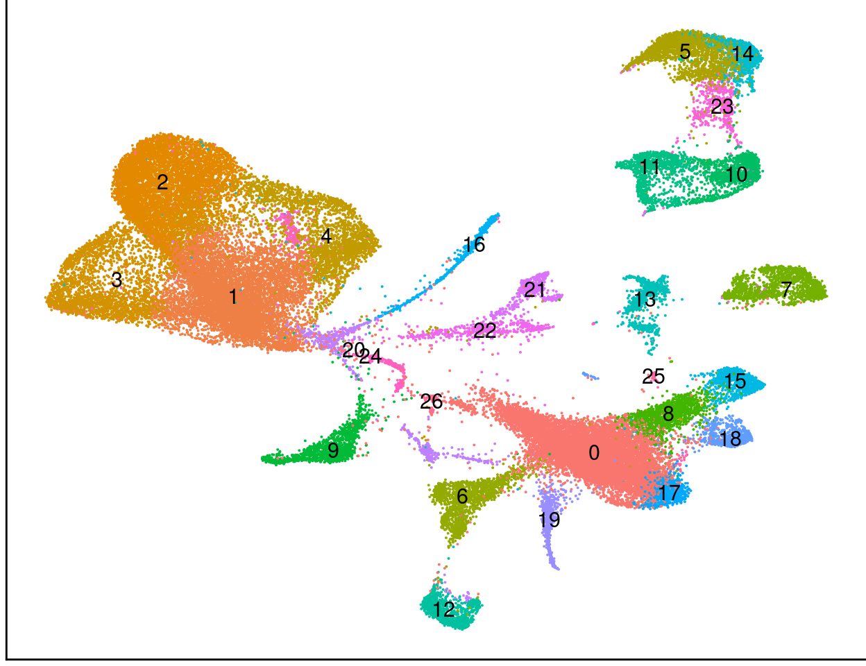
| Version | Author | Date |
|---|---|---|
| bdb871b | Pytrik Folkertsma | 2019-12-02 |
#save_plot("figures/figures_paper/main_figures/Figure_wolfrum/UMAP_wolfrum_clusters.pdf", p_clusters, base_width=6, base_height=5)#featureplots
#widht=13
#ucp2_fp <- featureplots_leg$UCP2 + scale_color_gradient(name='Expression', low='gray', #high='blue', guide='colorbar', limits=c(0,5)) + theme(plot.title=element_blank(), #legend.title=element_text(size=20), legend.text=element_text(size=20), legend.key.height = #unit(1.3, 'cm'))
#dcn_fp <- featureplots_noleg$DCN + theme(plot.title=element_blank())
adipoq <- FeaturePlot(wolfrum.predicted_labels, features='ADIPOQ') + NoLegend() + NoAxes() + theme(plot.title = element_text(size=20)) + scale_color_gradient(name='Expression', low='gray', high='blue', guide='colorbar', limits=c(0,5))Scale for 'colour' is already present. Adding another scale for
'colour', which will replace the existing scale.lipe <- FeaturePlot(wolfrum.predicted_labels, features='LIPE') + NoLegend() + NoAxes() + theme(plot.title = element_text(size=20)) + scale_color_gradient(name='Expression', low='gray', high='blue', guide='colorbar', limits=c(0,5))Scale for 'colour' is already present. Adding another scale for
'colour', which will replace the existing scale.apod <- FeaturePlot(wolfrum.predicted_labels, features='APOD') + NoLegend() + NoAxes() + theme(plot.title = element_text(size=20)) + scale_color_gradient(name='Expression', low='gray', high='blue', guide='colorbar', limits=c(0,5))Scale for 'colour' is already present. Adding another scale for
'colour', which will replace the existing scale.dcn <- FeaturePlot(wolfrum.predicted_labels, features='DCN') + NoAxes() + theme(plot.title = element_text(size=20), legend.text=element_text(size=20), legend.key.height = unit(1.3, 'cm')) + scale_color_gradient(name='Expression', low='gray', high='blue', guide='colorbar', limits=c(0,5)) Scale for 'colour' is already present. Adding another scale for
'colour', which will replace the existing scale.g <- plot_grid(
adipoq, lipe, apod, dcn, ncol=4, rel_widths=c(1, 1, 1, 1.3)
)
g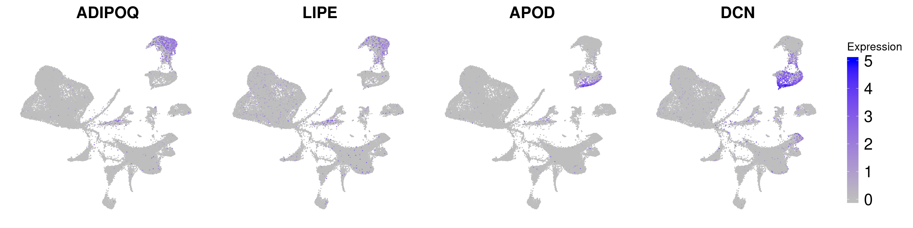
| Version | Author | Date |
|---|---|---|
| bdb871b | Pytrik Folkertsma | 2019-12-02 |
#save_plot("../figures/figures_paper/main_figures/Figure_wolfrum/featureplots.pdf", g, base_width=16, base_height=4)EBF2 and LEP
ebf2 <- FeaturePlot(wolfrum.predicted_labels, features='EBF2') + NoAxes() + theme(plot.title = element_text(size=20), legend.text=element_text(size=20), legend.key.height = unit(1.3, 'cm')) + scale_color_gradient(name='Expression', low='gray', high='blue', guide='colorbar') Scale for 'colour' is already present. Adding another scale for
'colour', which will replace the existing scale.pparg <- FeaturePlot(wolfrum.predicted_labels, features='PPARG') + NoAxes() + theme(plot.title = element_text(size=20), legend.text=element_text(size=20), legend.key.height = unit(1.3, 'cm')) + scale_color_gradient(name='Expression', low='gray', high='blue', guide='colorbar') Scale for 'colour' is already present. Adding another scale for
'colour', which will replace the existing scale.lep <- FeaturePlot(wolfrum.predicted_labels, features='LEP') + NoAxes() + theme(plot.title = element_text(size=20), legend.text=element_text(size=20), legend.key.height = unit(1.3, 'cm')) + scale_color_gradient(name='Expression', low='gray', high='blue', guide='colorbar') Scale for 'colour' is already present. Adding another scale for
'colour', which will replace the existing scale.ucp1 <- FeaturePlot(wolfrum.predicted_labels, features='UCP1') + NoAxes() + theme(plot.title = element_text(size=20), legend.text=element_text(size=20), legend.key.height = unit(1.3, 'cm')) + scale_color_gradient(name='Expression', low='gray', high='blue', guide='colorbar') Scale for 'colour' is already present. Adding another scale for
'colour', which will replace the existing scale.ebf2vln <- VlnPlot(wolfrum.predicted_labels, features='EBF2', group.by='RNA_snn_res.0.8', pt.size=-1) + NoLegend()
lepvln <- VlnPlot(wolfrum.predicted_labels, features='LEP', group.by='RNA_snn_res.0.8', pt.size=0.1) + NoLegend()
ucp1vln <- VlnPlot(wolfrum.predicted_labels, features='UCP1', group.by='RNA_snn_res.0.8', pt.size=0.1) + NoLegend()
ppargvln <- VlnPlot(wolfrum.predicted_labels, features='PPARG', group.by='RNA_snn_res.0.8', pt.size=0.1) + NoLegend()#save_plot("../figures/figures_paper/main_figures/Figure_wolfrum/ebf2.pdf", ebf2, base_width=5, base_height=4)
#save_plot("../figures/figures_paper/main_figures/Figure_wolfrum/ebf2vln.pdf", ebf2vln, base_width=6, base_height=2)
#save_plot("../figures/figures_paper/main_figures/Figure_wolfrum/pparg.pdf", pparg, base_width=5, base_height=4)
#save_plot("../figures/figures_paper/main_figures/Figure_wolfrum/ppargvln.pdf", ppargvln, base_width=6, base_height=2)
#save_plot("../figures/figures_paper/main_figures/Figure_wolfrum/ucp1.pdf", ucp1, base_width=5, base_height=4)
#save_plot("../figures/figures_paper/main_figures/Figure_wolfrum/ucp1vln.pdf", ucp1vln, base_width=6, base_height=2)
#save_plot("../figures/figures_paper/main_figures/Figure_wolfrum/lep.pdf", lep, base_width=5, base_height=4)
#save_plot("../figures/figures_paper/main_figures/Figure_wolfrum/lepvln.pdf", lepvln, base_width=5, base_height=2)UMAPPlot(wolfrum.predicted_labels, label=T, group.by='RNA_snn_res.0.8') 
| Version | Author | Date |
|---|---|---|
| bdb871b | Pytrik Folkertsma | 2019-12-02 |
VlnPlot(wolfrum.predicted_labels, features=c('EBF2', 'PPARG'), group.by='RNA_snn_res.0.8', pt.size=-1, ncol=1)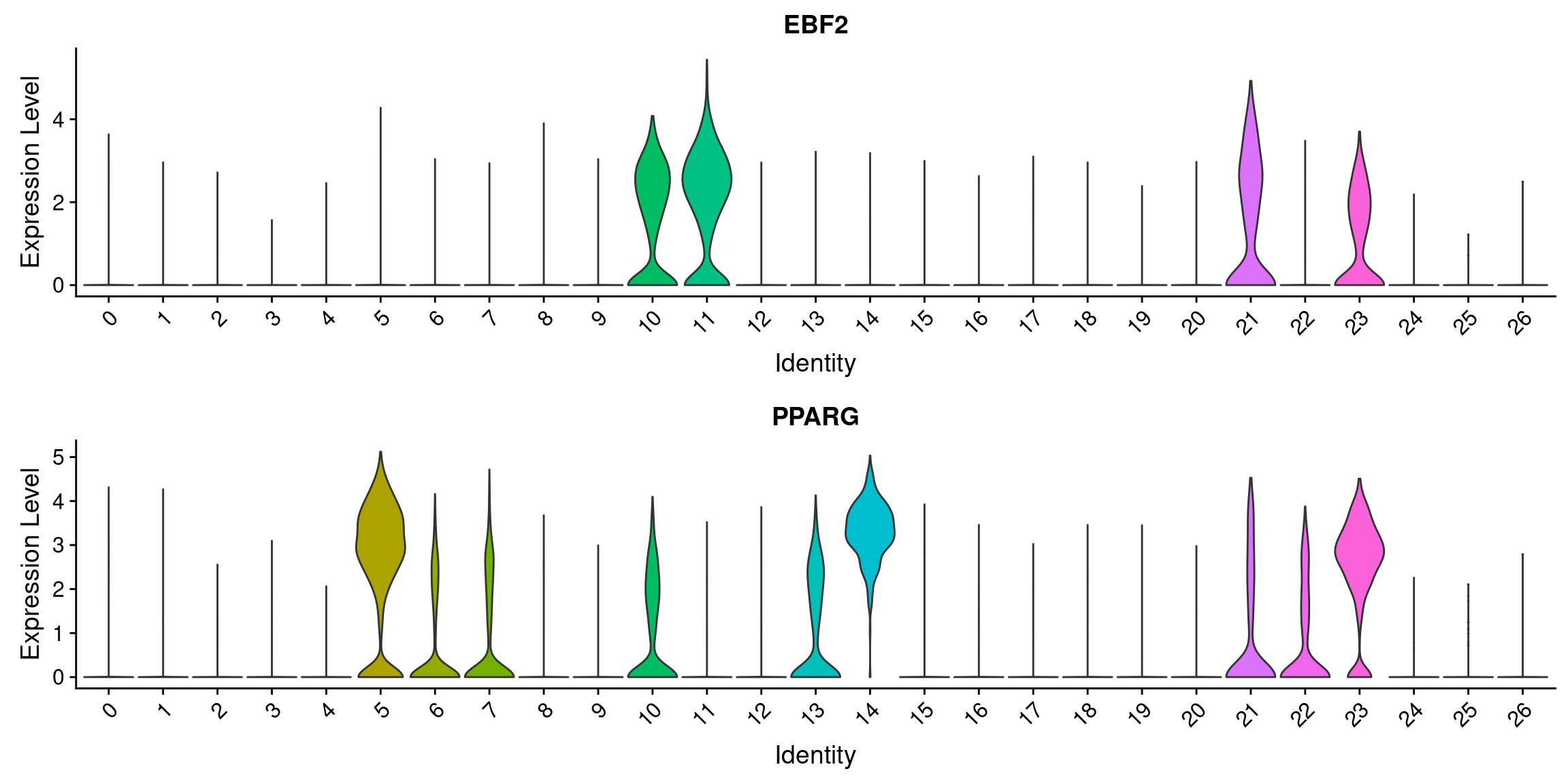
| Version | Author | Date |
|---|---|---|
| bdb871b | Pytrik Folkertsma | 2019-12-02 |
#EBF2 and PPARG
#PPARG: 5, 14, 23
#EBF2: 10, 11, 21, 23

new_labels <- unlist(lapply(wolfrum.predicted_labels@meta.data$RNA_snn_res.0.8, function(x){
  if (x %in% c(5, 14, 23, 10, 11, 21, 23)){
    return(x)
  } else {
    return(NA)
  }
}))

wolfrum.predicted_labels@meta.data['labels_clusters_preadipocytes'] <- new_labels
p <- UMAPPlot(wolfrum.predicted_labels, group.by='labels_clusters_preadipocytes', label=T) + theme(axis.text = element_blank(), axis.ticks = element_blank(), axis.title = element_blank(), plot.margin=grid::unit(c(0,0,0,0), "mm")) + NoLegend()
p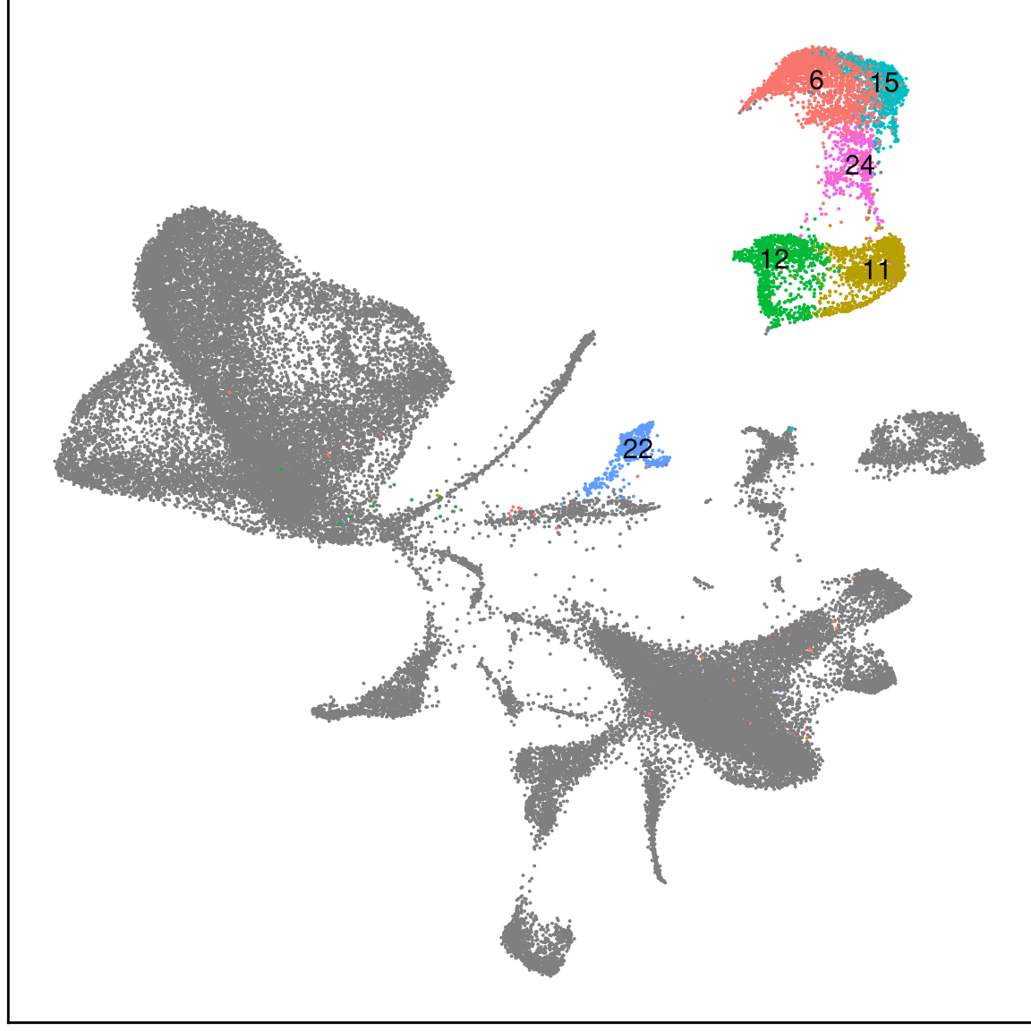
| Version | Author | Date |
|---|---|---|
| bdb871b | Pytrik Folkertsma | 2019-12-02 |
#save_plot("../figures/figures_paper/main_figures/Figure_wolfrum/UMAP_adipocyte_clusters2.pdf", p, base_width=6, base_height=5)ebf2 <- FeaturePlot(wolfrum.predicted_labels, features='EBF2', pt.size=0.5) + NoLegend() + NoAxes() + theme(plot.title = element_text(size=20)) + scale_color_gradient(name='Expression', low='gray', high='blue', guide='colorbar', limits=c(0,5))Scale for 'colour' is already present. Adding another scale for
'colour', which will replace the existing scale.pparg <- FeaturePlot(wolfrum.predicted_labels, features='PPARG', pt.size=0.5) + NoAxes() + theme(plot.title = element_text(size=20), legend.text=element_text(size=15), legend.key.height = unit(1.3, 'cm')) + scale_color_gradient(name='Expression', low='gray', high='blue', guide='colorbar', limits=c(0,5)) Scale for 'colour' is already present. Adding another scale for
'colour', which will replace the existing scale.g <- plot_grid(
ebf2, pparg, ncol=2, rel_widths = c(1, 1.3)
)
g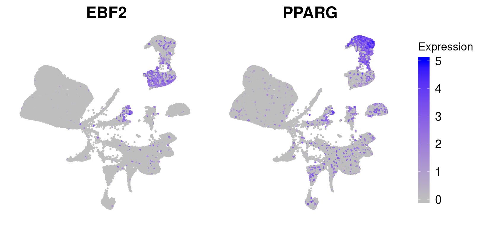
| Version | Author | Date |
|---|---|---|
| bdb871b | Pytrik Folkertsma | 2019-12-02 |
#save_plot("../figures/figures_paper/main_figures/Figure_wolfrum/EBF2_PPARG_ptsize0.5.pdf", g, base_width=8.5, base_height=4)plots <- VlnPlot(wolfrum.predicted_labels, features=c('ADIPOQ', 'LIPE', 'PLIN4', 'FABP4', 'ADIRF', 'APOD', 'MGP', 'DCN', 'CCDC80', 'PLAC9'), group.by='RNA_snn_res.0.8', pt.size=-1, combine=F)
for (i in 1:length(plots)){
if (i == length(plots)){
plots[[i]] <- plots[[i]] + NoLegend() +
theme(plot.title=element_blank(),
axis.title.y=element_blank(),
axis.line.x=element_blank(),
axis.text.x=element_text(angle=0, size=12),
plot.margin = unit(c(0, 0, 0, 0), "cm")) +
labs(x='Cluster')
} else {
plots[[i]] <- plots[[i]] + NoLegend() +
theme(plot.title=element_blank(),
axis.title.y=element_blank(),
axis.line.x=element_blank(),
axis.ticks.x=element_blank(),
axis.text.x=element_blank(),
axis.title.x=element_blank(),
plot.margin = unit(c(0, 0, 0, 0), "cm"))
}
}
vlnplts <- plot_grid(plotlist=plots, ncol=1, rel_heights=c(1,1,1,1,1,1,1,1,1,1.6))
vlnplts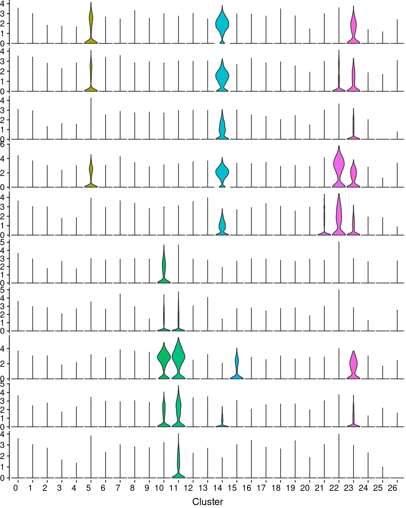
| Version | Author | Date |
|---|---|---|
| bdb871b | Pytrik Folkertsma | 2019-12-02 |
#save_plot("figures/figures_paper/main_figures/Figure_wolfrum/violinplots.pdf", p, base_width=6, base_height=8)Supplementary figure
integrated <- readRDS('output/seurat_objects/wolfrum/wolfrum.180831.integrated.rds')
sfig <- plot_grid(
  UMAPPlot(integrated, group.by='dataset'),
  UMAPPlot(integrated, group.by='State.labels', cols=colormap.branches),
  UMAPPlot(integrated, group.by='RNA_snn_res.0.8', label=T) + NoLegend(), ncol=2
)
sfig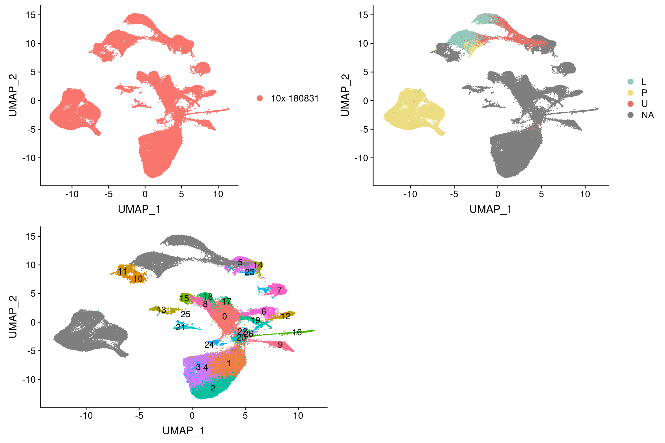
| Version | Author | Date |
|---|---|---|
| bdb871b | Pytrik Folkertsma | 2019-12-02 |
#save_plot("figures/figures_paper/supplementary_figures/wolfrum/integration.wolfrum.180831.pdf", sfig, base_width=12, base_height=8)
sessionInfo()R version 3.5.3 (2019-03-11)
Platform: x86_64-pc-linux-gnu (64-bit)
Running under: Storage
Matrix products: default
BLAS/LAPACK: /usr/lib64/libopenblas-r0.3.3.so
locale:
[1] LC_CTYPE=en_US.UTF-8 LC_NUMERIC=C
[3] LC_TIME=en_US.UTF-8 LC_COLLATE=en_US.UTF-8
[5] LC_MONETARY=en_US.UTF-8 LC_MESSAGES=en_US.UTF-8
[7] LC_PAPER=en_US.UTF-8 LC_NAME=C
[9] LC_ADDRESS=C LC_TELEPHONE=C
[11] LC_MEASUREMENT=en_US.UTF-8 LC_IDENTIFICATION=C
attached base packages:
[1] splines stats4 parallel stats graphics grDevices utils
[8] datasets methods base
other attached packages:
[1] DT_0.9 kableExtra_1.1.0 knitr_1.22
[4] tidyr_0.8.3 dplyr_0.8.0.1 cowplot_0.9.4
[7] monocle_2.8.0 DDRTree_0.1.5 irlba_2.3.3
[10] VGAM_1.1-1 ggplot2_3.1.0 Biobase_2.42.0
[13] BiocGenerics_0.28.0 Matrix_1.2-17 Seurat_3.1.1
loaded via a namespace (and not attached):
[1] backports_1.1.3 workflowr_1.2.0 plyr_1.8.4
[4] igraph_1.2.4 lazyeval_0.2.2 densityClust_0.3
[7] crosstalk_1.0.0 listenv_0.7.0 fastICA_1.2-1
[10] digest_0.6.18 htmltools_0.3.6 viridis_0.5.1
[13] gdata_2.18.0 fansi_0.4.0 magrittr_1.5
[16] cluster_2.1.0 ROCR_1.0-7 limma_3.36.5
[19] globals_0.12.4 readr_1.3.1 RcppParallel_4.4.4
[22] matrixStats_0.54.0 R.utils_2.8.0 docopt_0.6.1
[25] colorspace_1.4-1 rvest_0.3.3 ggrepel_0.8.0
[28] xfun_0.5 sparsesvd_0.1-4 crayon_1.3.4
[31] jsonlite_1.6 survival_2.43-3 zoo_1.8-5
[34] ape_5.3 glue_1.3.1 gtable_0.3.0
[37] webshot_0.5.1 leiden_0.3.1 future.apply_1.3.0
[40] scales_1.0.0 pheatmap_1.0.12 bibtex_0.4.2
[43] Rcpp_1.0.1 metap_1.1 viridisLite_0.3.0
[46] xtable_1.8-3 reticulate_1.11.1 rsvd_1.0.2
[49] SDMTools_1.1-221 tsne_0.1-3 htmlwidgets_1.3
[52] httr_1.4.0 FNN_1.1.3 gplots_3.0.1.1
[55] RColorBrewer_1.1-2 ica_1.0-2 pkgconfig_2.0.2
[58] R.methodsS3_1.7.1 uwot_0.1.4 utf8_1.1.4
[61] tidyselect_0.2.5 labeling_0.3 rlang_0.3.2
[64] reshape2_1.4.3 later_0.8.0 munsell_0.5.0
[67] tools_3.5.3 cli_1.1.0 ggridges_0.5.1
[70] evaluate_0.13 stringr_1.4.0 yaml_2.2.0
[73] npsurv_0.4-0 fs_1.2.7 fitdistrplus_1.0-14
[76] caTools_1.17.1.2 purrr_0.3.2 RANN_2.6.1
[79] pbapply_1.4-0 future_1.15.0 nlme_3.1-140
[82] whisker_0.3-2 mime_0.6 slam_0.1-45
[85] R.oo_1.22.0 xml2_1.2.0 compiler_3.5.3
[88] rstudioapi_0.10 plotly_4.8.0 png_0.1-7
[91] lsei_1.2-0 tibble_2.1.1 stringi_1.4.3
[94] lattice_0.20-38 HSMMSingleCell_0.114.0 pillar_1.3.1
[97] combinat_0.0-8 Rdpack_0.10-1 lmtest_0.9-36
[100] RcppAnnoy_0.0.13 data.table_1.12.0 bitops_1.0-6
[103] gbRd_0.4-11 httpuv_1.5.0 R6_2.4.0
[106] promises_1.0.1 KernSmooth_2.23-15 gridExtra_2.3
[109] codetools_0.2-16 MASS_7.3-51.4 gtools_3.8.1
[112] assertthat_0.2.1 rprojroot_1.3-2 withr_2.1.2
[115] qlcMatrix_0.9.7 sctransform_0.2.0 hms_0.4.2
[118] grid_3.5.3 rmarkdown_1.12 Rtsne_0.15
[121] git2r_0.25.2 shiny_1.2.0