Last updated: 2019-03-29

Checks: 6 0

Knit directory: 10x-adipocyte-analysis/

This reproducible R Markdown analysis was created with workflowr (version 1.2.0). The Report tab describes the reproducibility checks that were applied when the results were created. The Past versions tab lists the development history.

R Markdown file: up-to-date

Great! Since the R Markdown file has been committed to the Git repository, you know the exact version of the code that produced these results.

Environment: empty

Great job! The global environment was empty. Objects defined in the global environment can affect the analysis in your R Markdown file in unknown ways. For reproduciblity it’s best to always run the code in an empty environment.

Seed: set.seed(20181026)

The command set.seed(20181026) was run prior to running the code in the R Markdown file. Setting a seed ensures that any results that rely on randomness, e.g. subsampling or permutations, are reproducible.

Session information: recorded

Great job! Recording the operating system, R version, and package versions is critical for reproducibility.

Cache: none

Nice! There were no cached chunks for this analysis, so you can be confident that you successfully produced the results during this run.

Repository version: 398f133

Great! You are using Git for version control. Tracking code development and connecting the code version to the results is critical for reproducibility. The version displayed above was the version of the Git repository at the time these results were generated.

Note that you need to be careful to ensure that all relevant files for the analysis have been committed to Git prior to generating the results (you can use wflow_publish or wflow_git_commit). workflowr only checks the R Markdown file, but you know if there are other scripts or data files that it depends on. Below is the status of the Git repository when the results were generated:


Ignored files:
    Ignored:    analysis/figure/
    Ignored:    figures/
    Ignored:    output/bulk_analysis/
    Ignored:    output/markergenes/
    Ignored:    output/monocle/
    Ignored:    output/seurat_objects/
    Ignored:    output/velocyto/
    Ignored:    output/wgcna/
    Ignored:    tables/

Untracked files:
    Untracked:  analysis/.ipynb_checkpoints/velocyto_notebook_180831-checkpoint.ipynb
    Untracked:  analysis/10x-180831-monocle-featureselection.Rmd
    Untracked:  analysis/10x-180831-monocle.Rmd

Unstaged changes:
    Modified:   analysis/10x-180831-general-analysis.Rmd
    Modified:   analysis/velocyto_notebook_180831.ipynb
    Modified:   code/run-monocle.R

Note that any generated files, e.g. HTML, png, CSS, etc., are not included in this status report because it is ok for generated content to have uncommitted changes.

There are no past versions. Publish this analysis with wflow_publish() to start tracking its development.

library(Seurat)

Loading required package: ggplot2

Loading required package: cowplot


Attaching package: 'cowplot'

The following object is masked from 'package:ggplot2':

    ggsave

Loading required package: Matrix

library(monocle)

Loading required package: Biobase

Loading required package: BiocGenerics

Loading required package: parallel


Attaching package: 'BiocGenerics'

The following objects are masked from 'package:parallel':

    clusterApply, clusterApplyLB, clusterCall, clusterEvalQ,
    clusterExport, clusterMap, parApply, parCapply, parLapply,
    parLapplyLB, parRapply, parSapply, parSapplyLB

The following objects are masked from 'package:Matrix':

    colMeans, colSums, rowMeans, rowSums, which

The following objects are masked from 'package:stats':

    IQR, mad, sd, var, xtabs

The following objects are masked from 'package:base':

    anyDuplicated, append, as.data.frame, basename, cbind,
    colMeans, colnames, colSums, dirname, do.call, duplicated,
    eval, evalq, Filter, Find, get, grep, grepl, intersect,
    is.unsorted, lapply, lengths, Map, mapply, match, mget, order,
    paste, pmax, pmax.int, pmin, pmin.int, Position, rank, rbind,
    Reduce, rowMeans, rownames, rowSums, sapply, setdiff, sort,
    table, tapply, union, unique, unsplit, which, which.max,
    which.min

Welcome to Bioconductor

    Vignettes contain introductory material; view with
    'browseVignettes()'. To cite Bioconductor, see
    'citation("Biobase")', and for packages 'citation("pkgname")'.

Loading required package: VGAM

Loading required package: stats4

Loading required package: splines

Loading required package: DDRTree

Loading required package: irlba

library(colorspace)

seurobj <- readRDS('output/seurat_objects/180831/10x-180831')

Colors

hcl_palettes(plot = TRUE)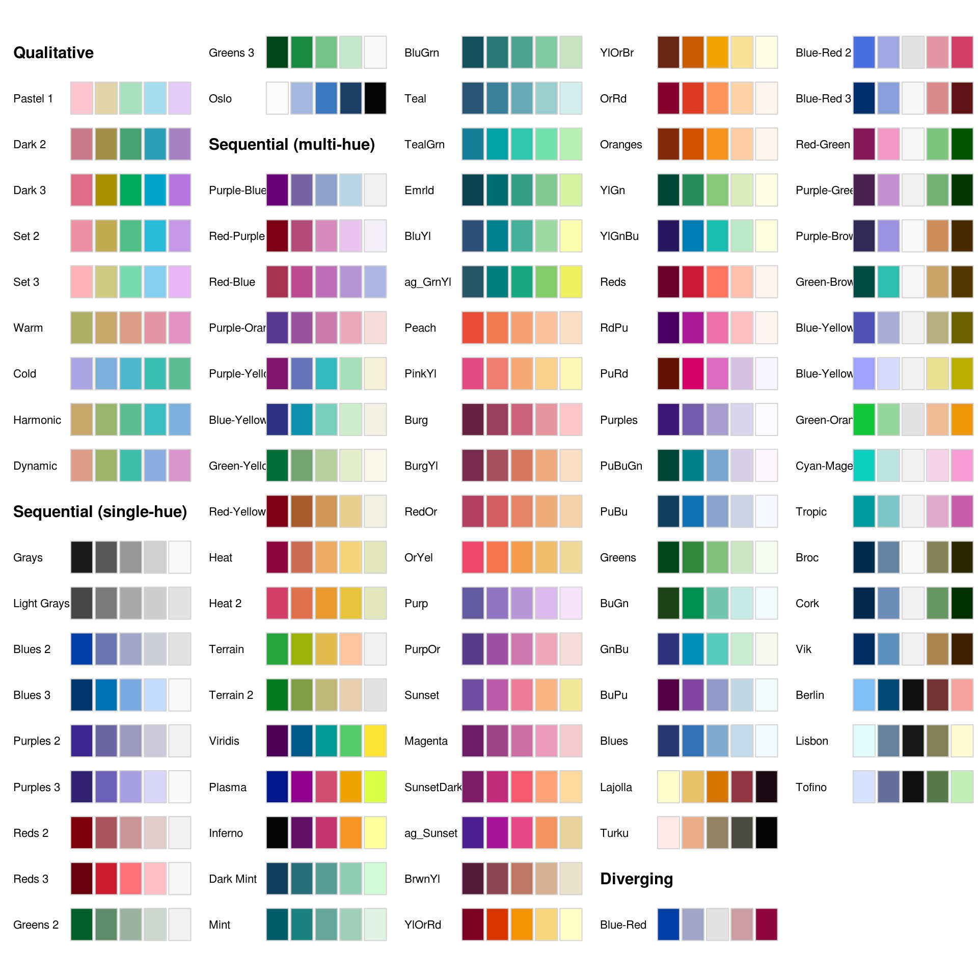

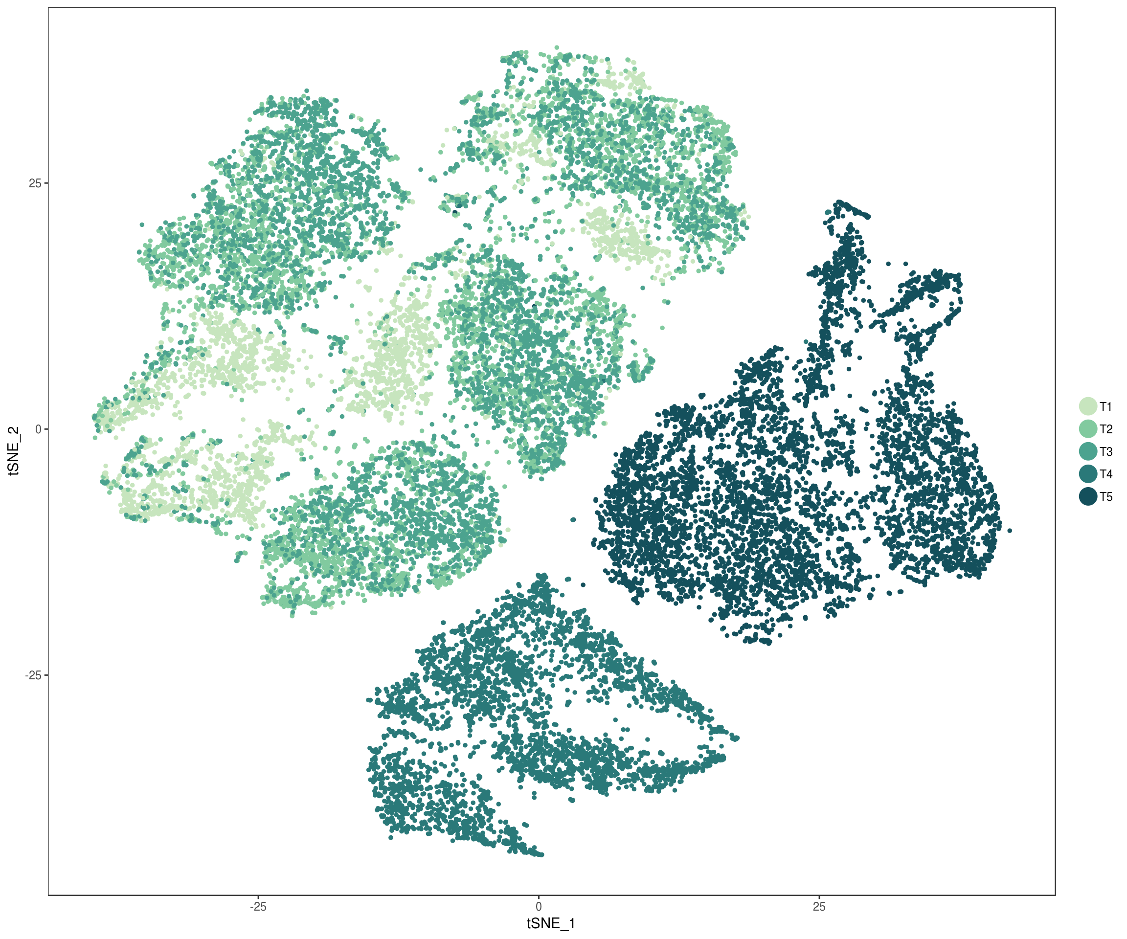
Timepoint colors

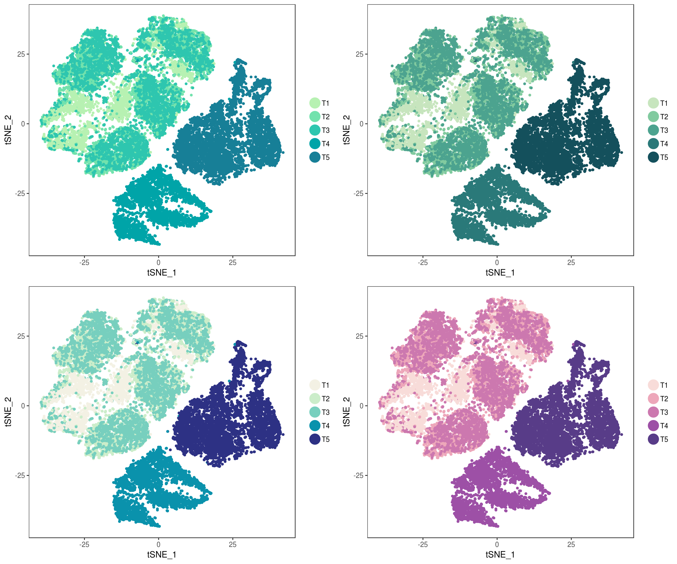
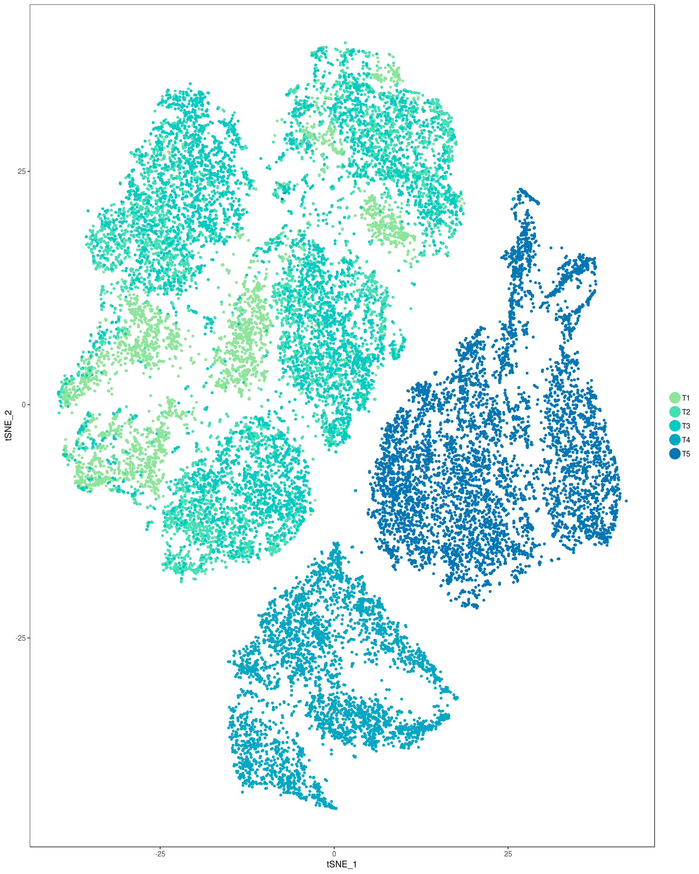
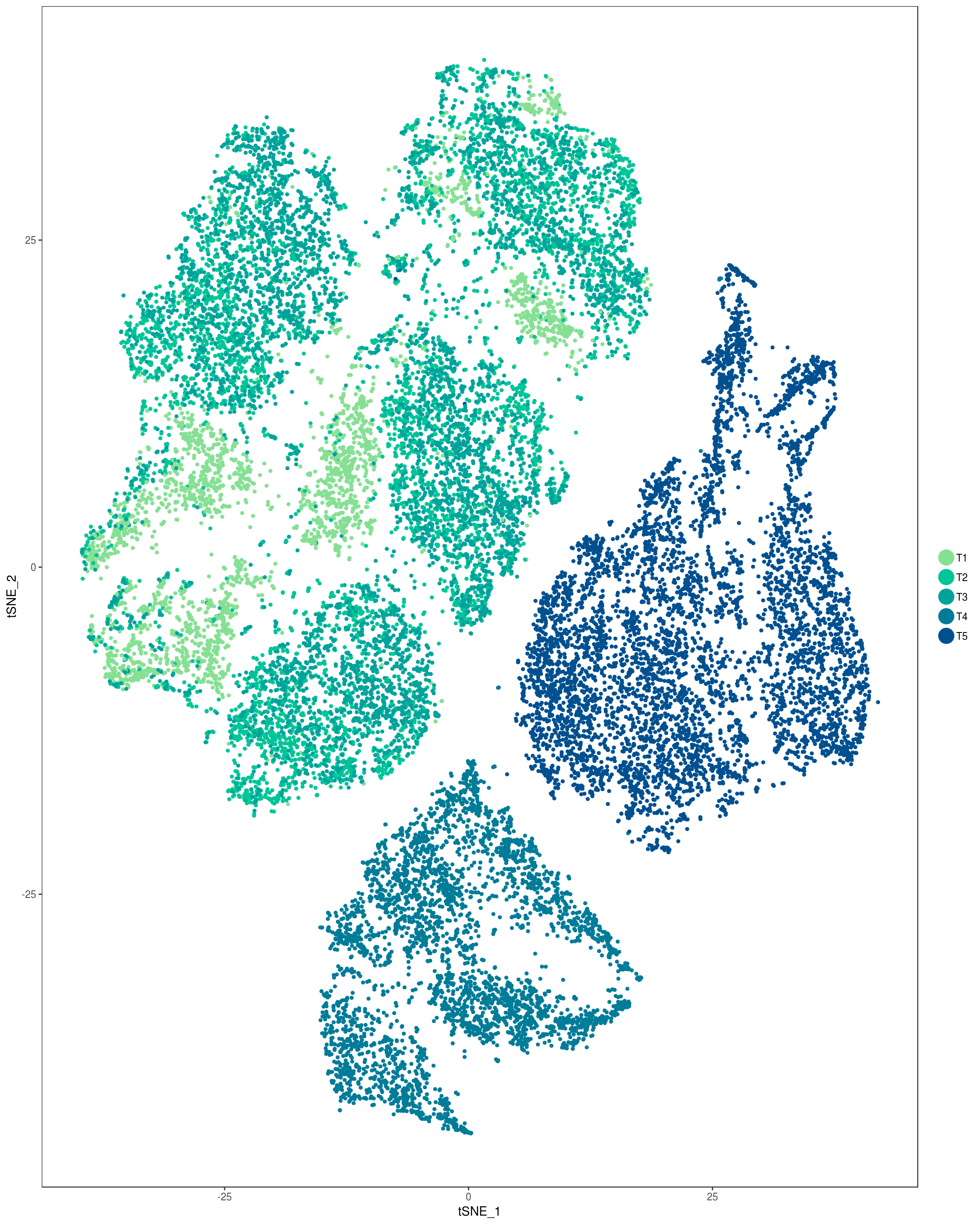
plot_grid(
  TSNEPlot(seurobj, group.by='timepoint', pt.size=1, colors.use=rev(sequential_hcl(5, palette='TealGrn'))),
  TSNEPlot(seurobj, group.by='timepoint', pt.size=1, colors.use=rev(sequential_hcl(5, palette='BluGrn'))),
  TSNEPlot(seurobj, group.by='timepoint', pt.size=1, colors.use=rev(sequential_hcl(5, palette='Blue Yellow'))),
  TSNEPlot(seurobj, group.by='timepoint', pt.size=1, colors.use=rev(sequential_hcl(5, palette='PurpOr')))
)

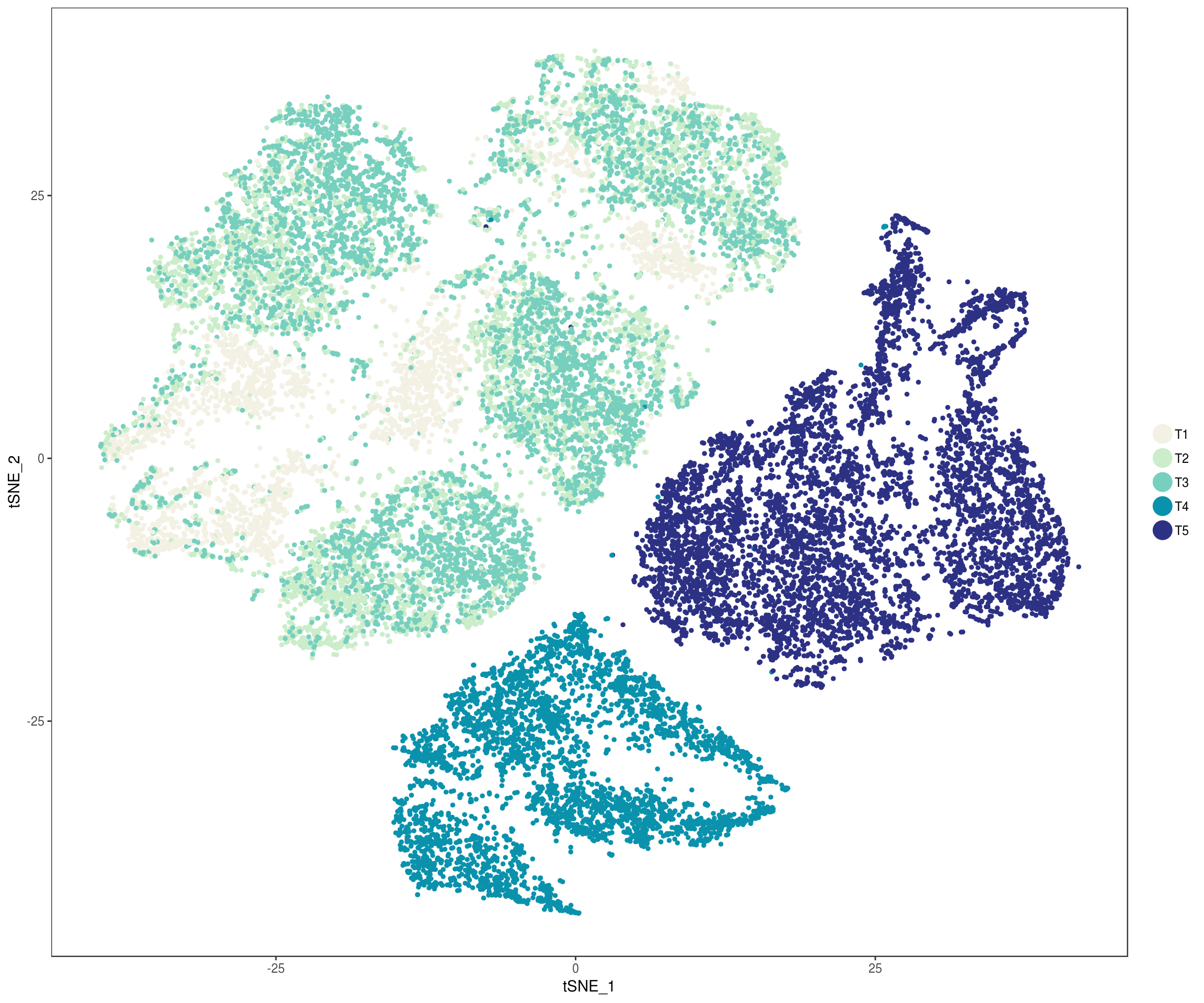
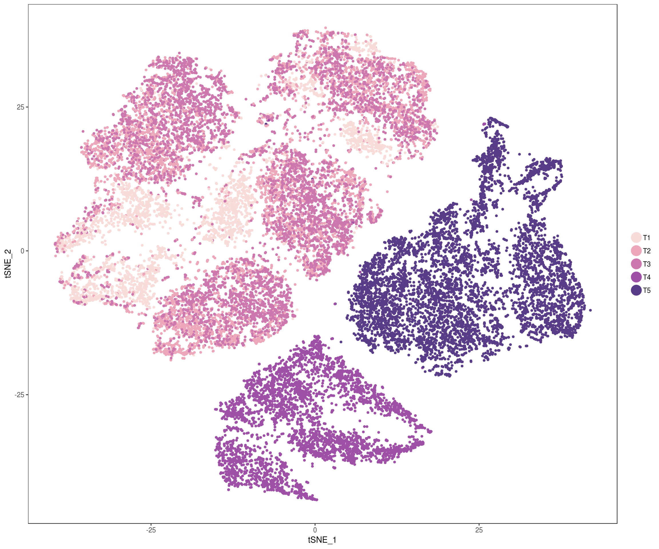
Custom colors timepoints

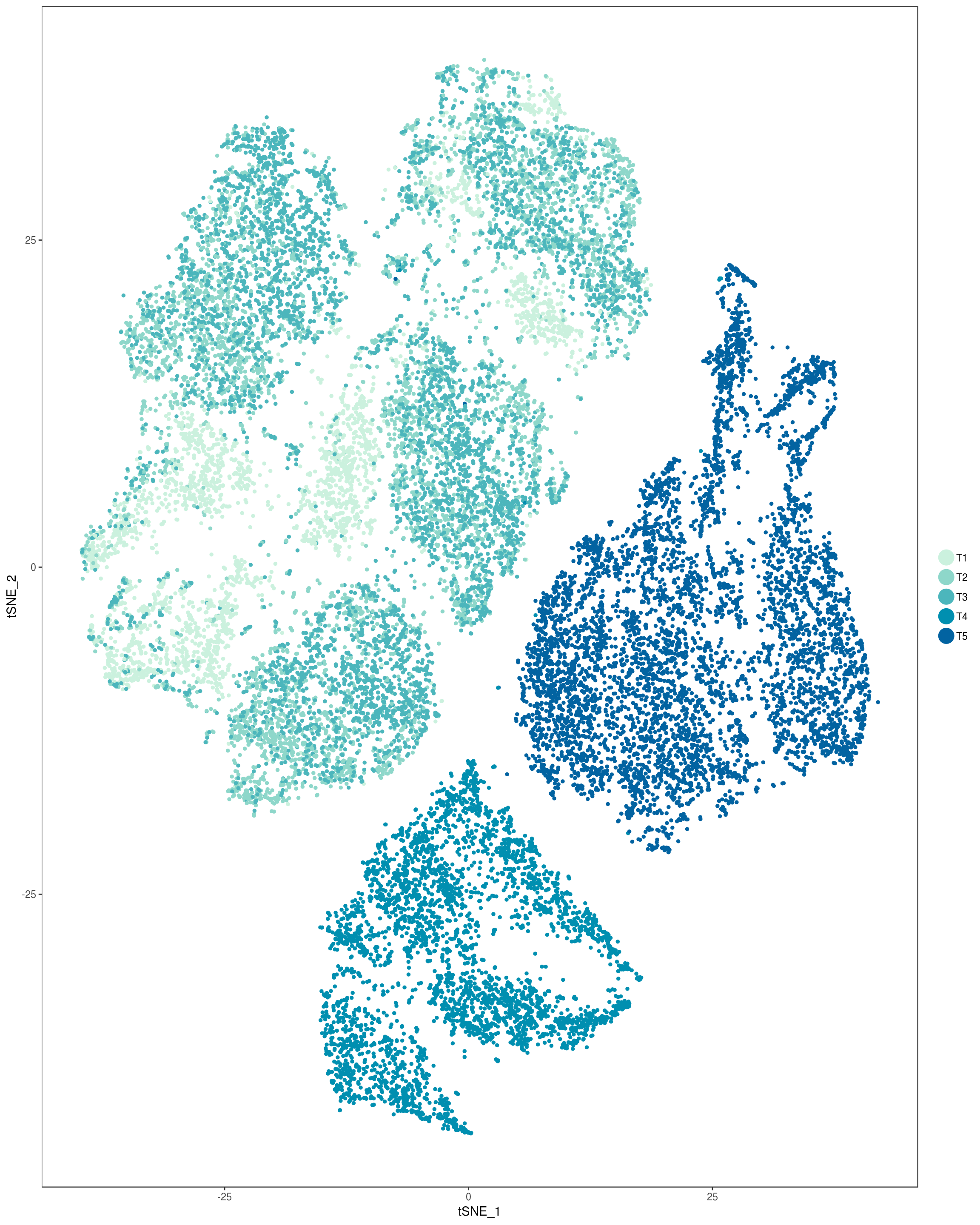
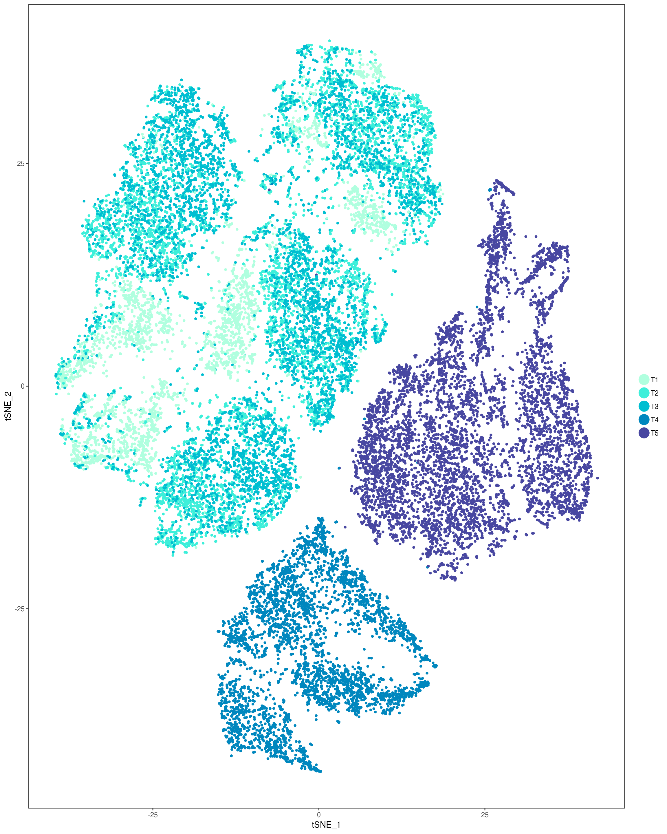
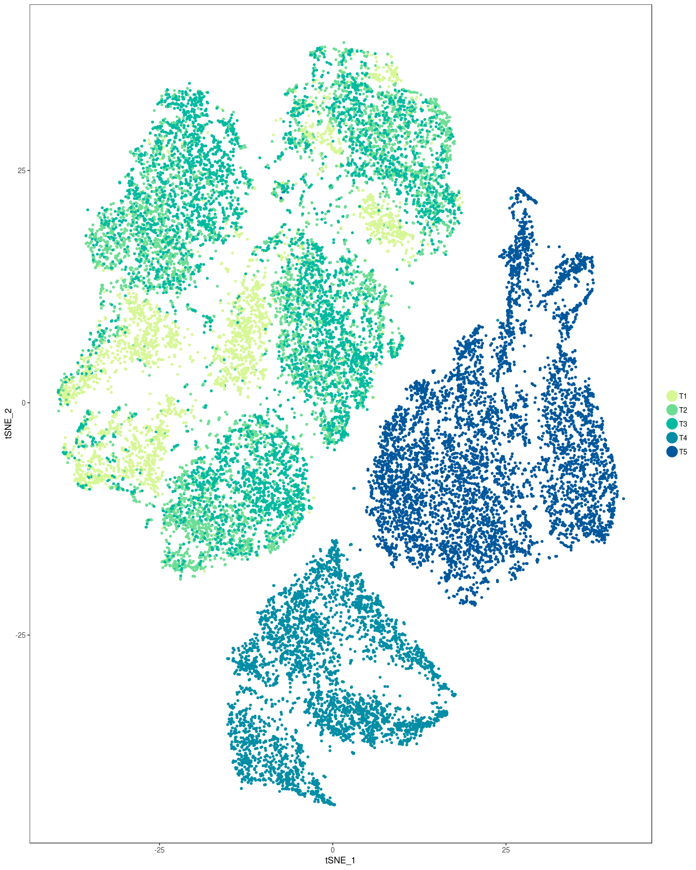
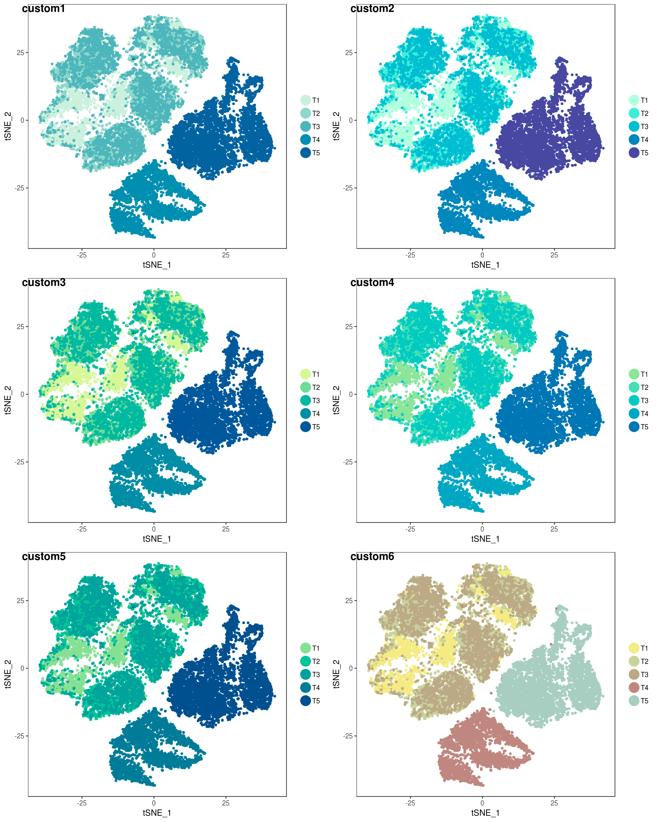
plot_grid(
  TSNEPlot(seurobj, group.by='timepoint', pt.size=1, colors.use=rev(c('#0263A1', '#008FB0', '#4CB6BC', '#8ED7CA', '#CBF1DE'))),
  TSNEPlot(seurobj, group.by='timepoint', pt.size=1, colors.use=rev(c('#4847A1', '#0087BE', '#00BED1', '#3DEFDA', '#B0FFDF'))),
  TSNEPlot(seurobj, group.by='timepoint', pt.size=1, colors.use=rev(c('#00589C','#008DA5', '#00B9A1', '#6DDD95', '#D7F797'))),
  TSNEPlot(seurobj, group.by='timepoint', pt.size=1, colors.use=rev(c('#0077B5', '#00A7C3', '#00CAC2', '#42E0B4', '#8CE599'))),
  TSNEPlot(seurobj, group.by='timepoint', pt.size=1, colors.use=rev(c('#005090','#007C98','#00A39B','#00C598','#86E094'))),
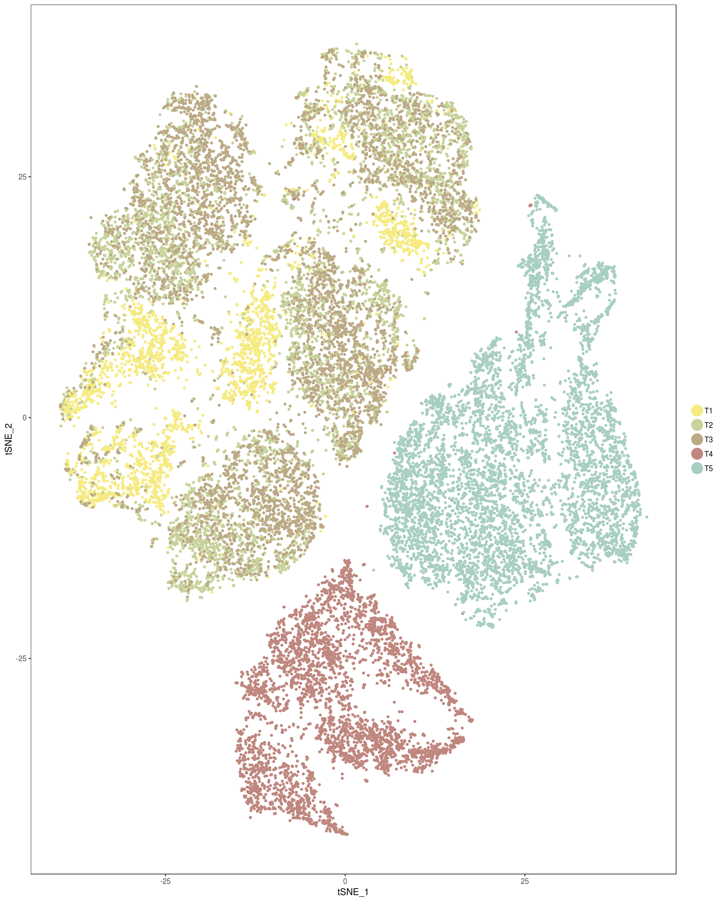
   TSNEPlot(seurobj, group.by='timepoint', pt.size=1, colors.use=c('#f5eb82','#c8d29b','#bca986','#bf877f','#a8cec2')), ncol=2, labels=c('custom1', 'custom2', 'custom3', 'custom4', 'custom5', 'custom6')
)

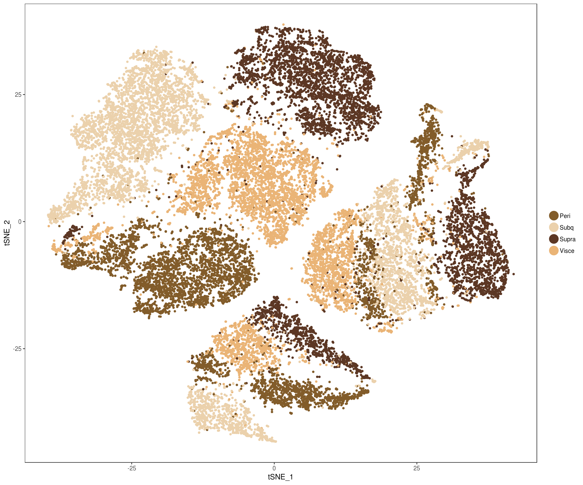
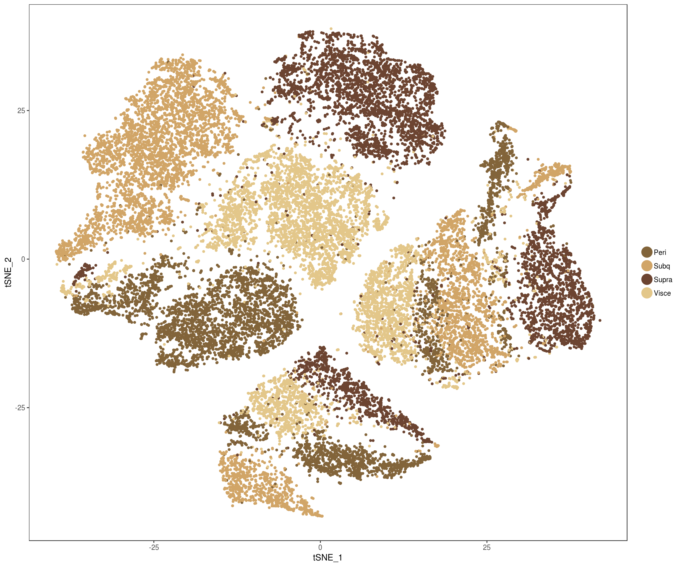
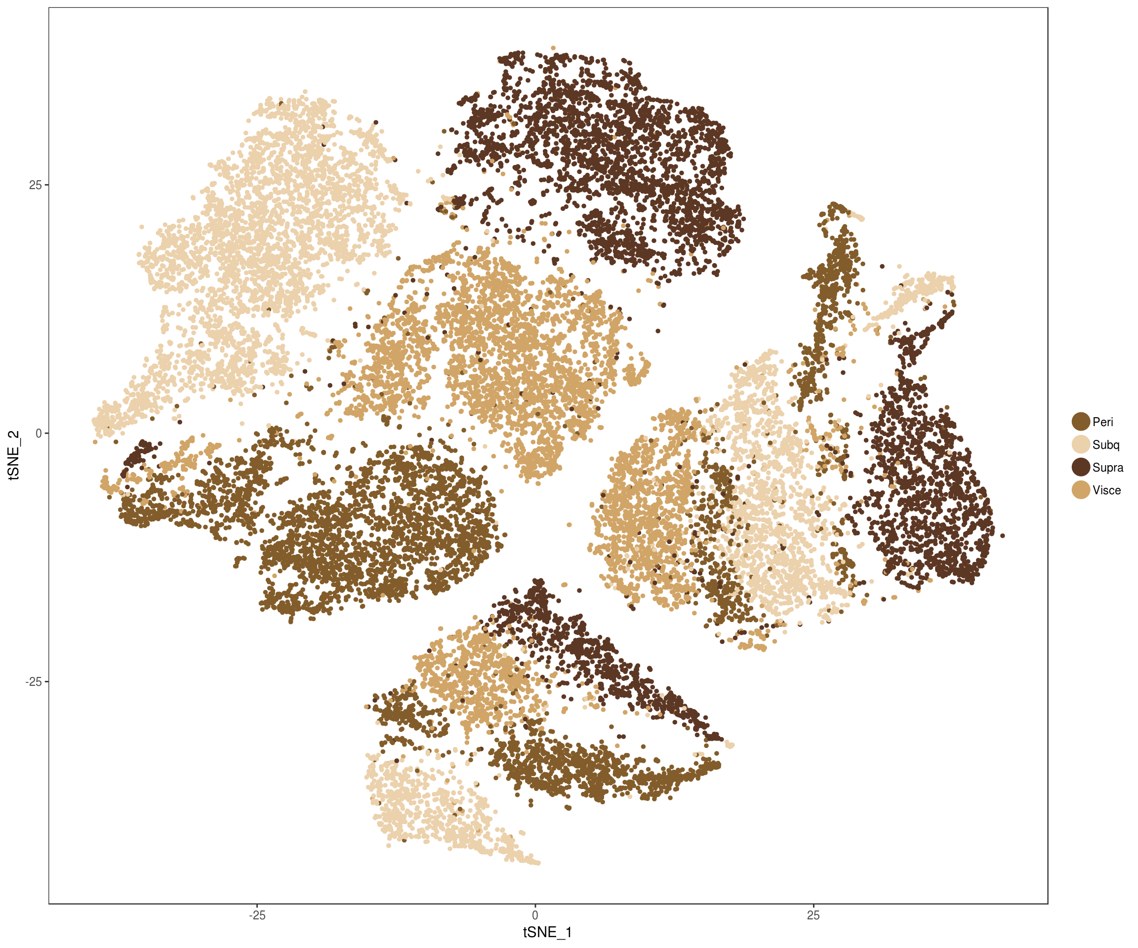
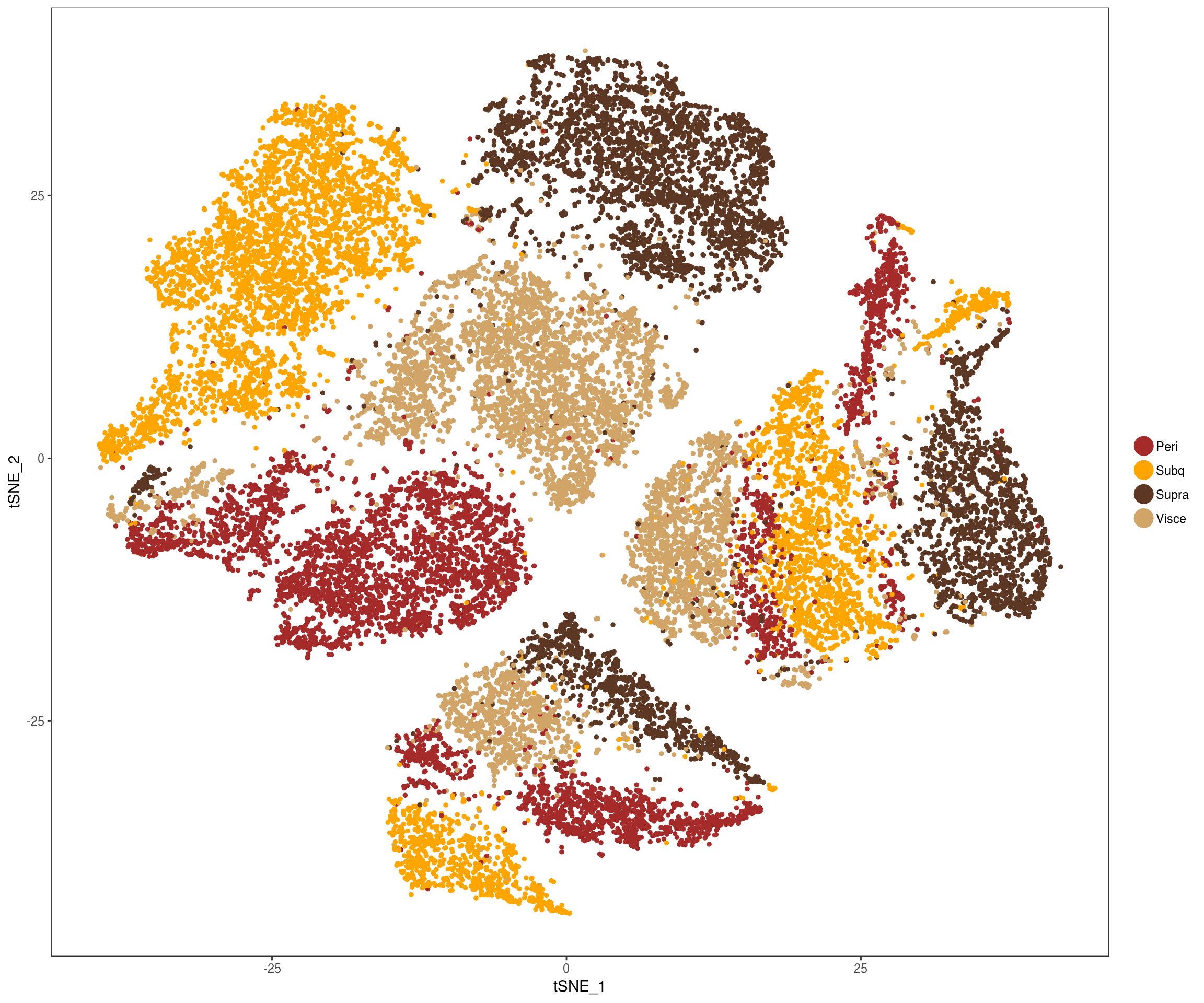
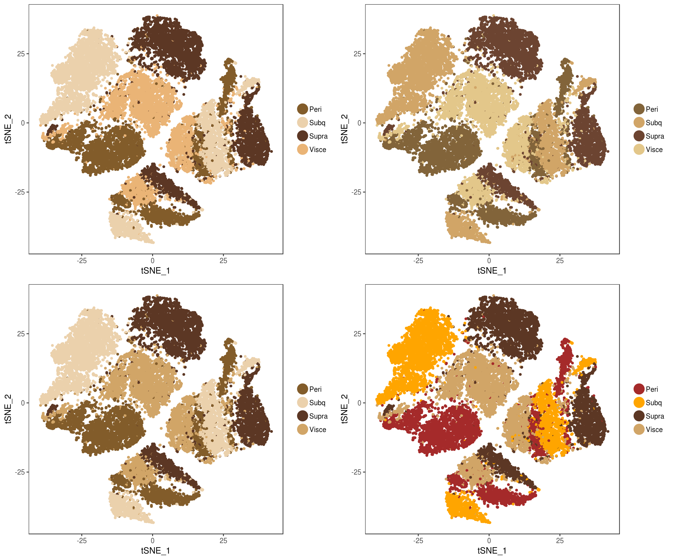
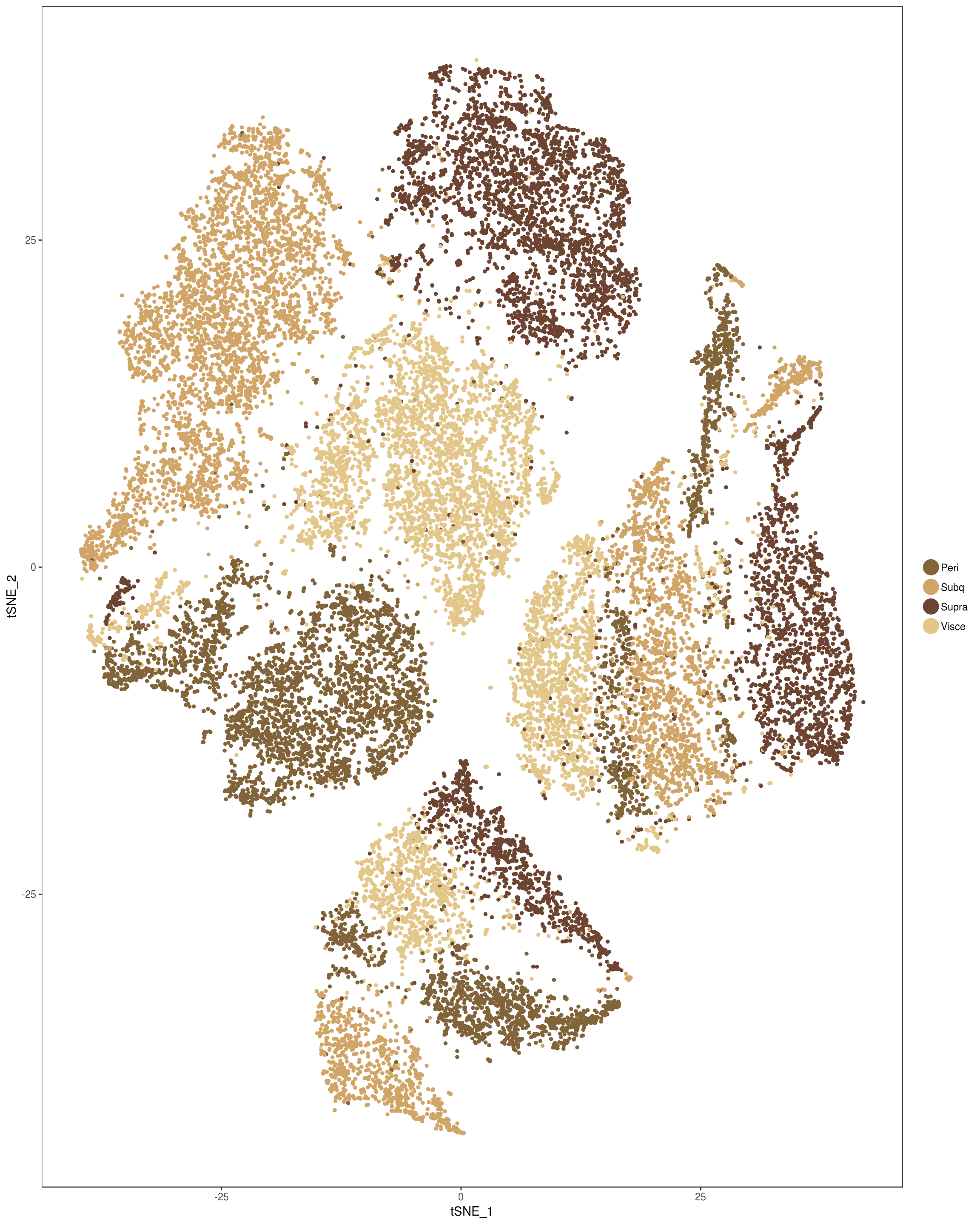
Depots

plot_grid(
  TSNEPlot(seurobj, group.by='depot', pt.size=1, colors.use=c('#825c2a', '#ebd1ac', '#5c3724', '#eab476')),
  TSNEPlot(seurobj, group.by='depot', pt.size=1, colors.use=c('#82643a', '#d1a567', '#6c4431', '#e3c78a')),
  TSNEPlot(seurobj, group.by='depot', pt.size=1, colors.use=c('#825c2a', '#ebd1ac', '#5c3724', '#d1a567')),
  TSNEPlot(seurobj, group.by='depot', pt.size=1, colors.use=c('brown', 'orange', '#5c3724', '#d1a567')),
  ncol=2
)

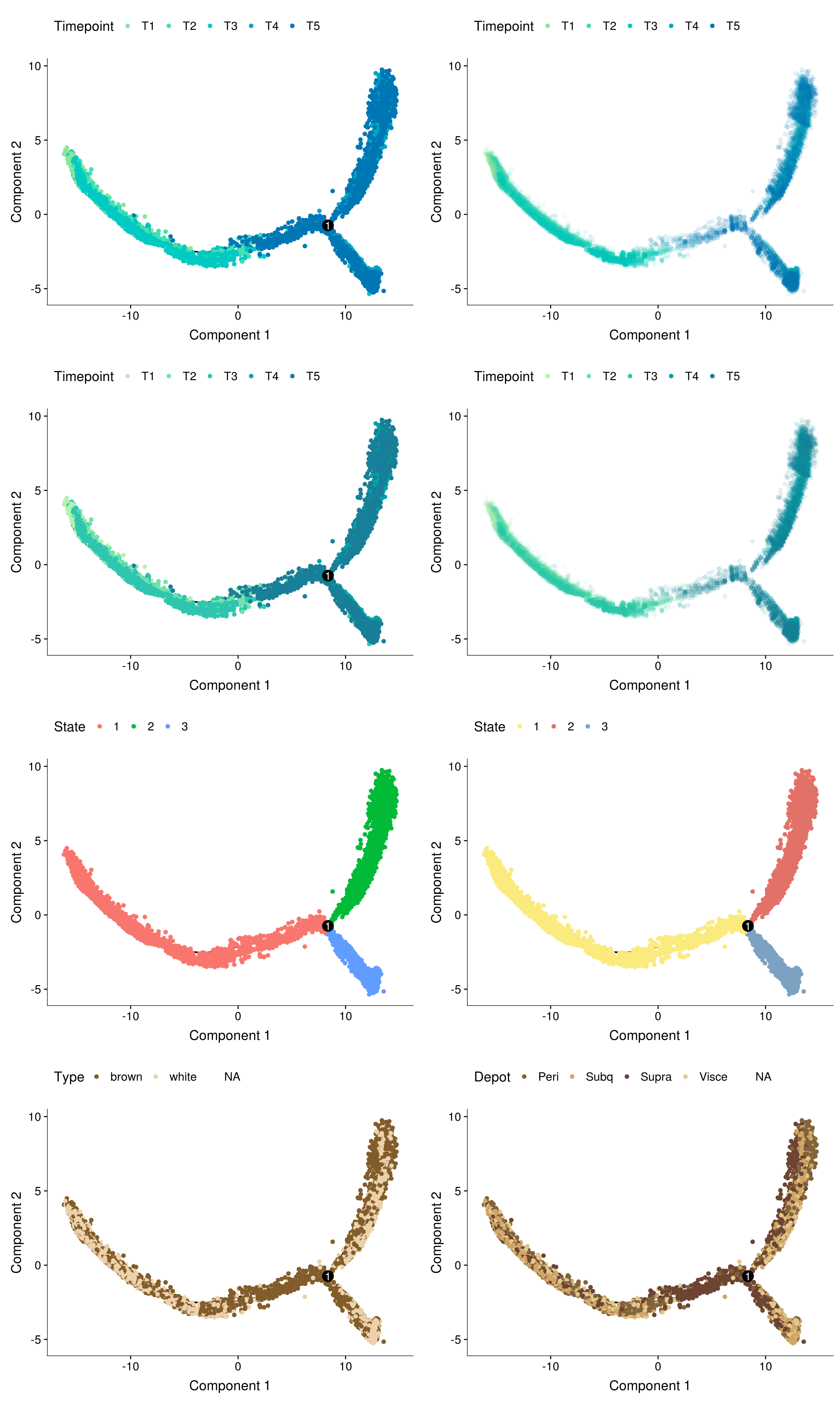
Monocle

cds <- readRDS('output/monocle/180831/monocle_T1T2T3_T4T5_res1.5/10x-180831-monocle-metadata')

plot_grid(
  plot_cell_trajectory(cds, color_by='timepoint') + scale_color_manual(values=rev(c('#0077B5', '#00A7C3', '#00CAC2', '#42E0B4', '#8CE599')), name = "Timepoint"),
  plot_cell_trajectory(cds, color_by='timepoint') + geom_point(color='white', size=5) + geom_point(aes(colour=timepoint), alpha=0.1) + scale_color_manual(values=rev(c('#0077B5', '#00A7C3', '#00CAC2', '#42E0B4', '#8CE599')), name = "Timepoint"),
  plot_cell_trajectory(cds, color_by='timepoint') + scale_color_manual(values=rev(sequential_hcl(5, palette='TealGrn')), name = "Timepoint"),
  plot_cell_trajectory(cds, color_by='timepoint') + geom_point(color='white', size=5) + geom_point(aes(colour=timepoint), alpha=0.1) + scale_color_manual(values=rev(sequential_hcl(5, palette='TealGrn')), name = "Timepoint"),
  plot_cell_trajectory(cds),
  plot_cell_trajectory(cds) + scale_color_manual(values=c('#fbea7d', '#e27268', '#7ba2c3'), name='State'),
  plot_cell_trajectory(cds, color_by='type') + scale_color_manual(values=c('#825c2a', '#ebd1ac'), name='Type'),
  plot_cell_trajectory(cds, color_by='depot') + scale_color_manual(values=c('#82643a', '#d1a567', '#6c4431', '#e3c78a'), name='Depot'),
  ncol=2
)

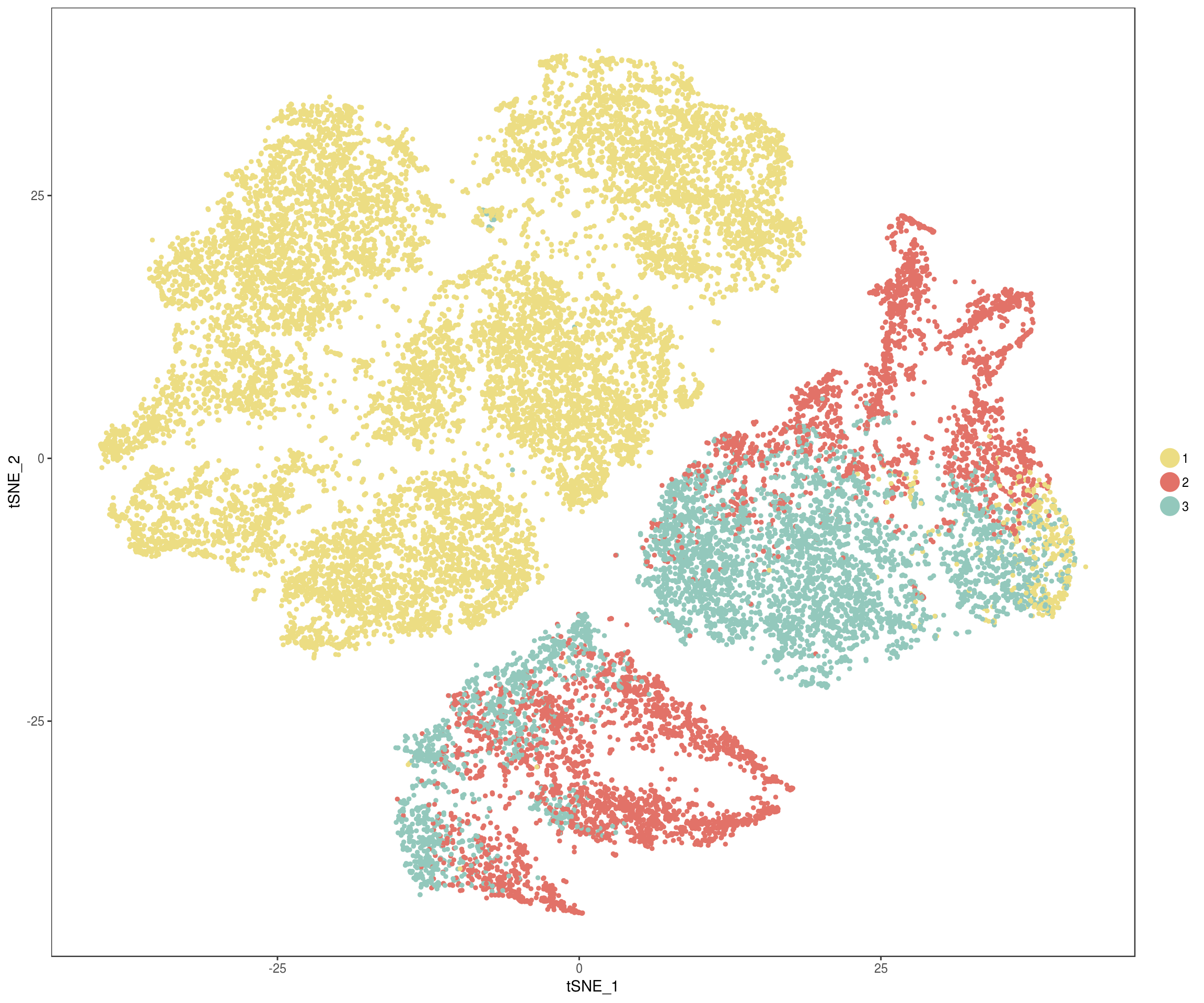
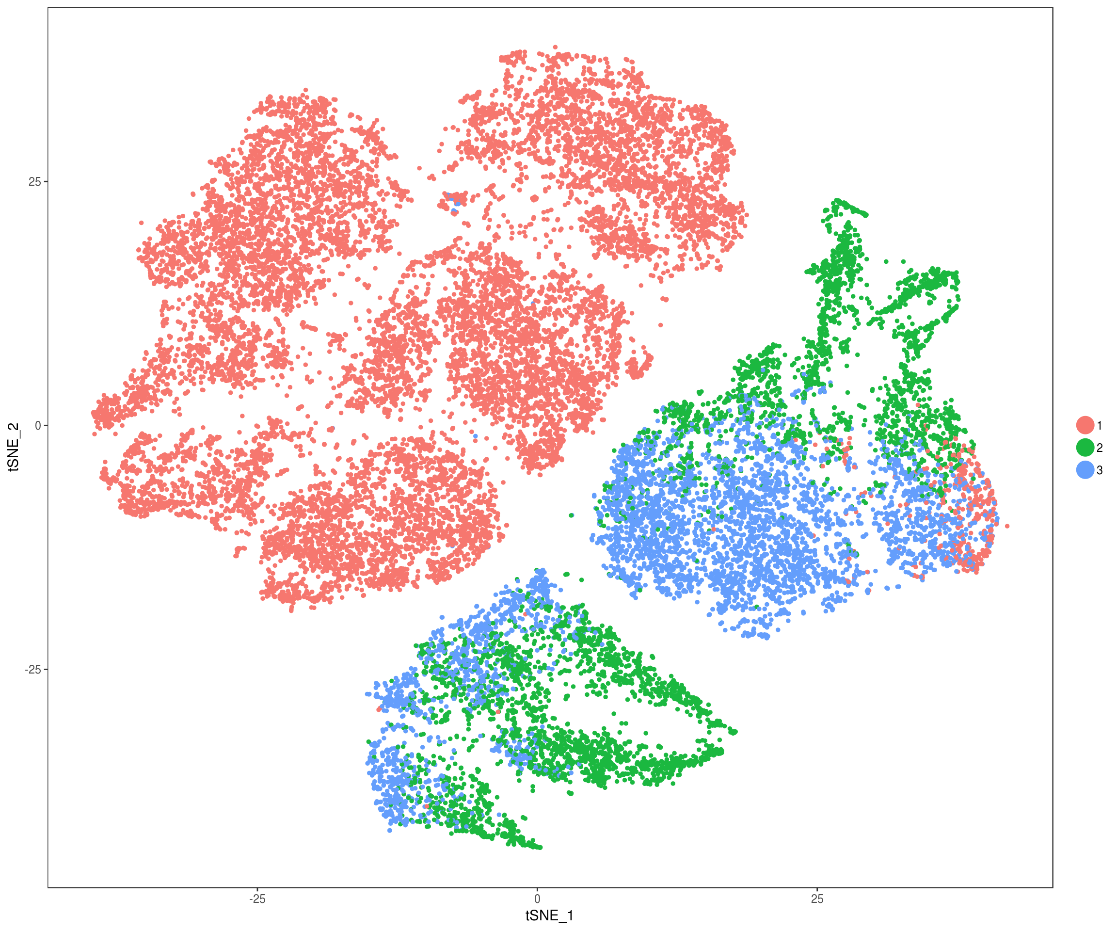
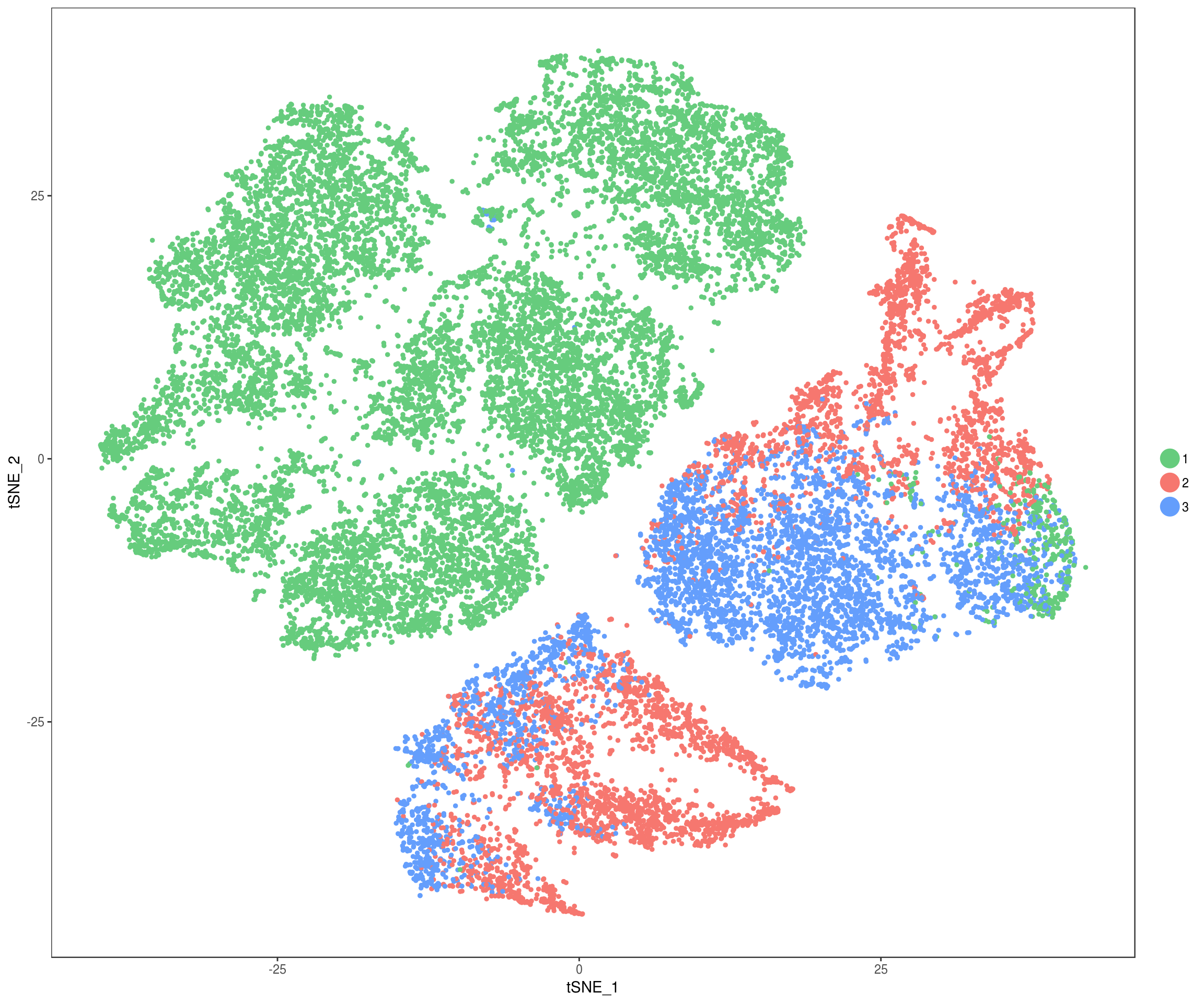
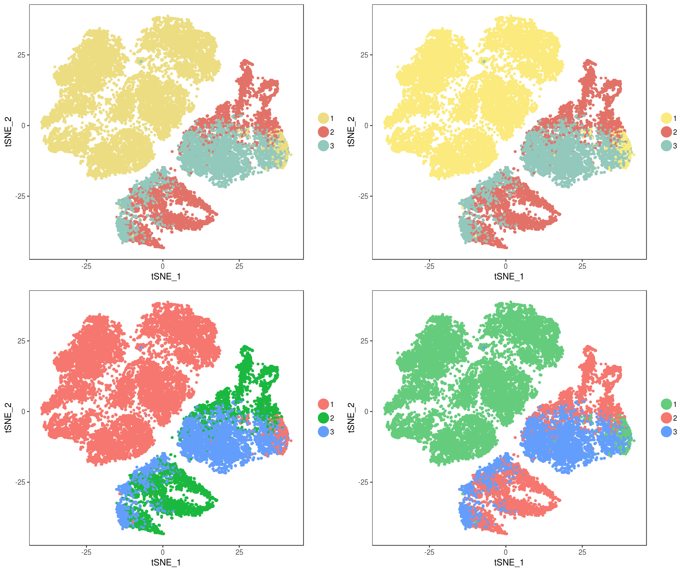
Monocle predictions in Seurat tSNE

plot_grid(
  TSNEPlot(seurobj, group.by='State.old', pt.size=1, colors.use=c('#ecdd83', '#e27268', '#93c8bc')),
  TSNEPlot(seurobj, group.by='State.old', pt.size=1, colors.use=c('#fbea7d', '#e27268', '#93c8bc')),
  TSNEPlot(seurobj, group.by='State.old', pt.size=1, colors.use=c('#f6776f', '#1bb840', '#649efc')),
  TSNEPlot(seurobj, group.by='State.old', pt.size=1, colors.use=c('#66cc7d', '#f6776f', '#649efc')),
  ncol=2
)

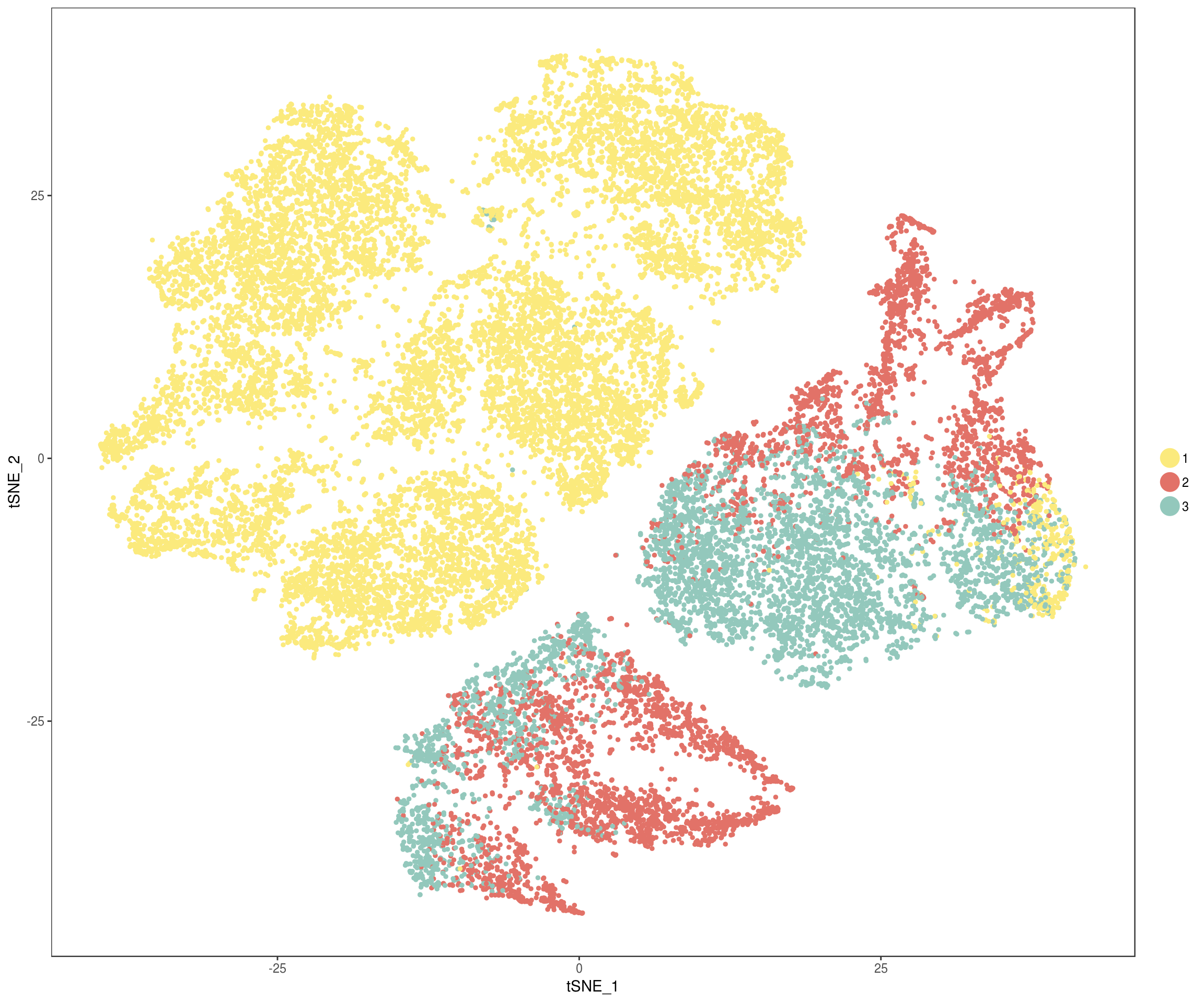
Final figures

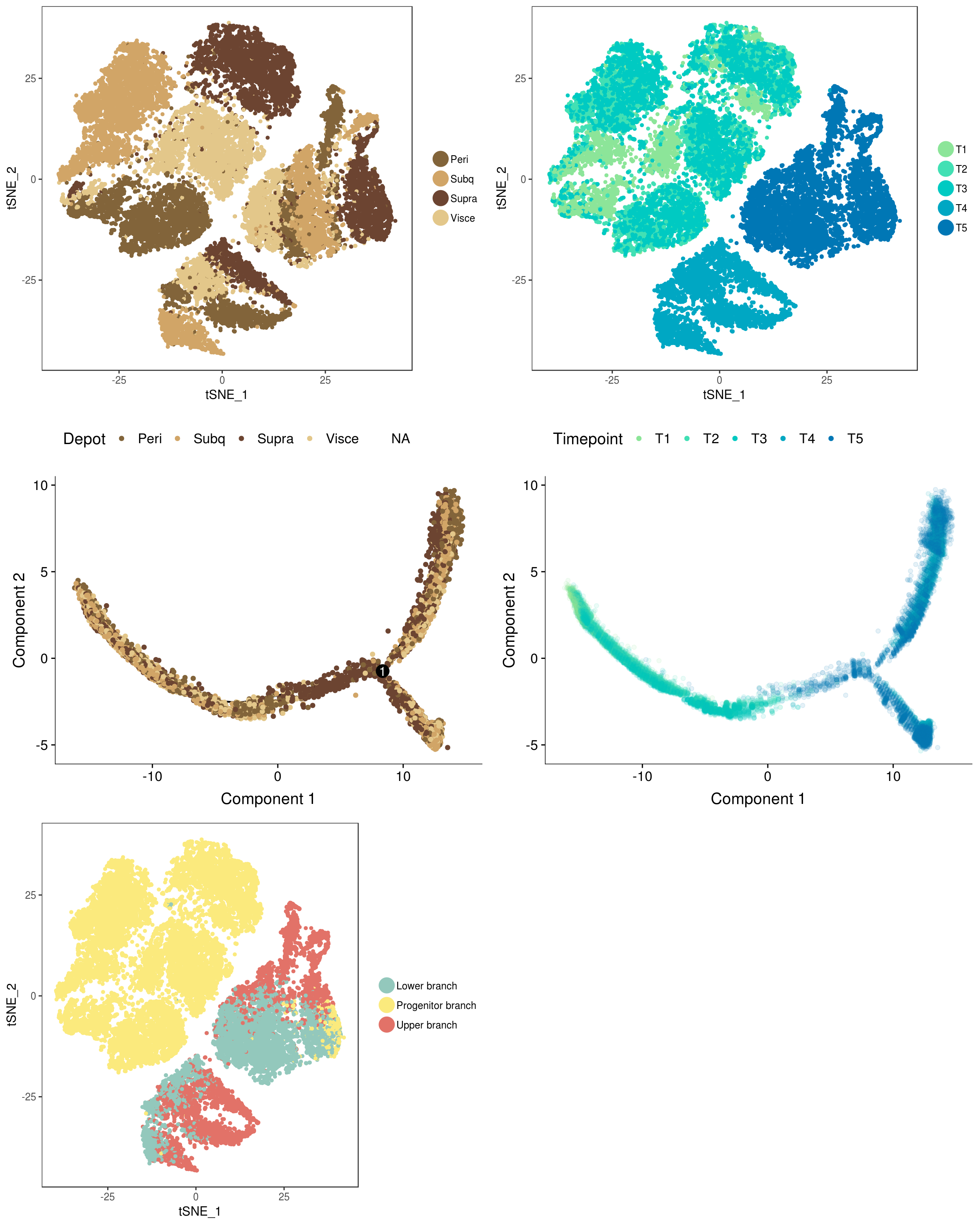
plot_grid(
  TSNEPlot(seurobj, group.by='depot', pt.size=1, colors.use=c('#82643a', '#d1a567', '#6c4431', '#e3c78a')),
  TSNEPlot(seurobj, group.by='timepoint', pt.size=1, colors.use=rev(c('#0077B5', '#00A7C3', '#00CAC2', '#42E0B4', '#8CE599'))),
  plot_cell_trajectory(cds, color_by='depot') + scale_color_manual(values=c('#82643a', '#d1a567', '#6c4431', '#e3c78a'), name='Depot'),
  plot_cell_trajectory(cds, color_by='timepoint') + geom_point(color='white', size=5) + geom_point(aes(colour=timepoint), alpha=0.1) + scale_color_manual(values=rev(c('#0077B5', '#00A7C3', '#00CAC2', '#42E0B4', '#8CE599')), name = "Timepoint"),
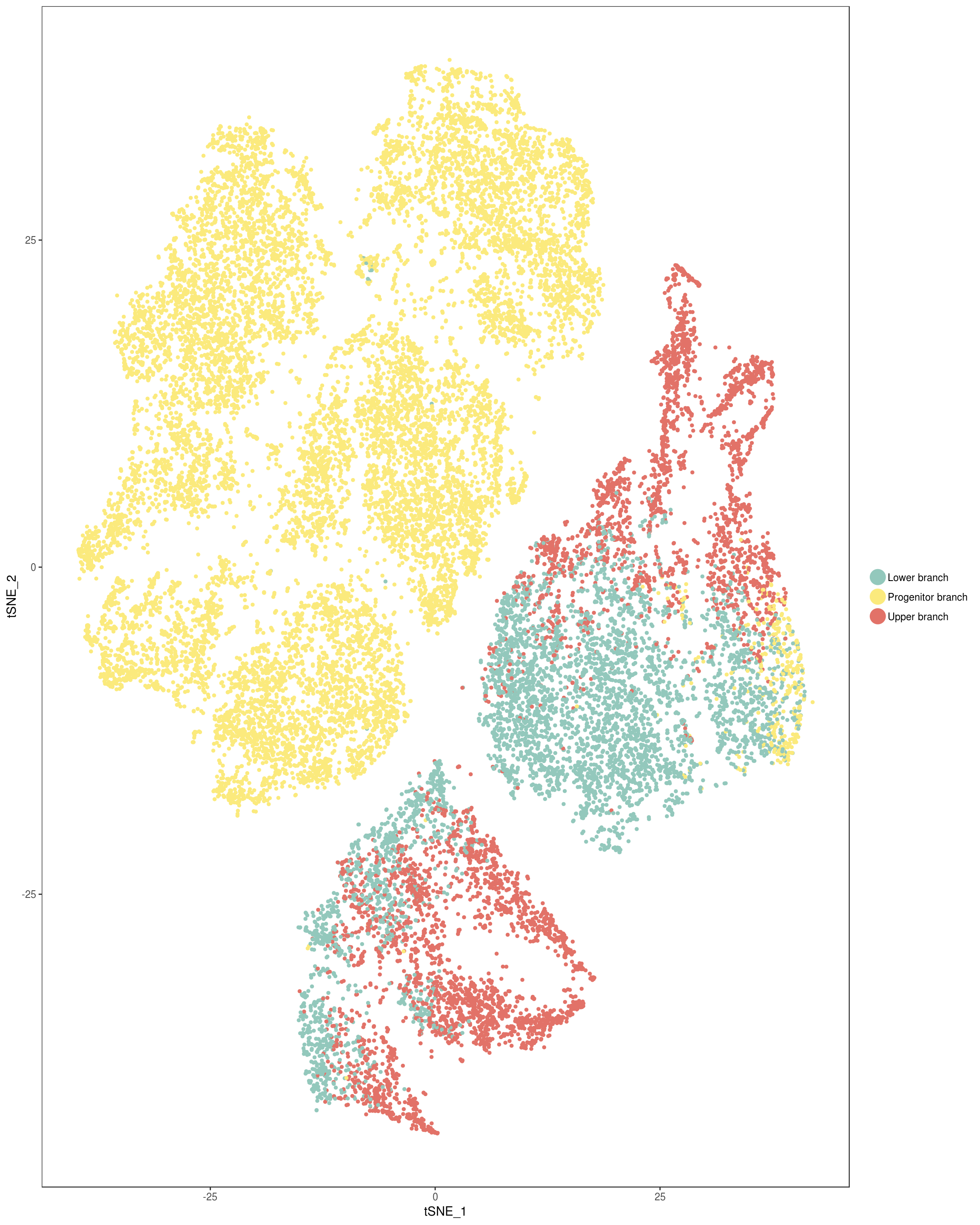
  TSNEPlot(seurobj, group.by='State.labels', pt.size=1, colors.use=c('#93c8bc', '#fbea7d', '#e27268')),
  ncol=2
)

sessionInfo()

R version 3.5.3 (2019-03-11)
Platform: x86_64-pc-linux-gnu (64-bit)
Running under: Storage

Matrix products: default
BLAS/LAPACK: /usr/lib64/libopenblas-r0.3.3.so

locale:
 [1] LC_CTYPE=en_US.UTF-8       LC_NUMERIC=C              
 [3] LC_TIME=en_US.UTF-8        LC_COLLATE=en_US.UTF-8    
 [5] LC_MONETARY=en_US.UTF-8    LC_MESSAGES=en_US.UTF-8   
 [7] LC_PAPER=en_US.UTF-8       LC_NAME=C                 
 [9] LC_ADDRESS=C               LC_TELEPHONE=C            
[11] LC_MEASUREMENT=en_US.UTF-8 LC_IDENTIFICATION=C       

attached base packages:
 [1] splines   stats4    parallel  stats     graphics  grDevices utils    
 [8] datasets  methods   base     

other attached packages:
 [1] colorspace_1.4-1    monocle_2.8.0       DDRTree_0.1.5      
 [4] irlba_2.3.3         VGAM_1.1-1          Biobase_2.42.0     
 [7] BiocGenerics_0.28.0 Seurat_2.3.4        Matrix_1.2-17      
[10] cowplot_0.9.4       ggplot2_3.1.0      

loaded via a namespace (and not attached):
  [1] Rtsne_0.15             class_7.3-15           modeltools_0.2-22     
  [4] ggridges_0.5.1         mclust_5.4.3           rprojroot_1.3-2       
  [7] htmlTable_1.13.1       base64enc_0.1-3        fs_1.2.7              
 [10] rstudioapi_0.10        proxy_0.4-23           npsurv_0.4-0          
 [13] ggrepel_0.8.0          flexmix_2.3-15         bit64_0.9-7           
 [16] mvtnorm_1.0-10         codetools_0.2-16       R.methodsS3_1.7.1     
 [19] docopt_0.6.1           lsei_1.2-0             robustbase_0.93-4     
 [22] knitr_1.22             jsonlite_1.6           Formula_1.2-3         
 [25] workflowr_1.2.0        ica_1.0-2              cluster_2.0.7-1       
 [28] kernlab_0.9-27         png_0.1-7              R.oo_1.22.0           
 [31] pheatmap_1.0.12        compiler_3.5.3         httr_1.4.0            
 [34] backports_1.1.3        assertthat_0.2.1       lazyeval_0.2.2        
 [37] limma_3.36.5           lars_1.2               acepack_1.4.1         
 [40] htmltools_0.3.6        tools_3.5.3            igraph_1.2.4          
 [43] gtable_0.3.0           glue_1.3.1             reshape2_1.4.3        
 [46] RANN_2.6.1             dplyr_0.8.0.1          Rcpp_1.0.1            
 [49] slam_0.1-45            trimcluster_0.1-2.1    gdata_2.18.0          
 [52] ape_5.3                nlme_3.1-137           iterators_1.0.10      
 [55] fpc_2.1-11.1           gbRd_0.4-11            lmtest_0.9-36         
 [58] xfun_0.5               stringr_1.4.0          gtools_3.8.1          
 [61] DEoptimR_1.0-8         MASS_7.3-51.1          zoo_1.8-5             
 [64] scales_1.0.0           doSNOW_1.0.16          RColorBrewer_1.1-2    
 [67] yaml_2.2.0             reticulate_1.11.1      pbapply_1.4-0         
 [70] gridExtra_2.3          rpart_4.1-13           segmented_0.5-3.0     
 [73] fastICA_1.2-1          latticeExtra_0.6-28    stringi_1.4.3         
 [76] foreach_1.4.4          checkmate_1.9.1        caTools_1.17.1.2      
 [79] densityClust_0.3       bibtex_0.4.2           matrixStats_0.54.0    
 [82] Rdpack_0.10-1          SDMTools_1.1-221       rlang_0.3.2           
 [85] pkgconfig_2.0.2        dtw_1.20-1             prabclus_2.2-7        
 [88] bitops_1.0-6           qlcMatrix_0.9.7        evaluate_0.13         
 [91] lattice_0.20-38        ROCR_1.0-7             purrr_0.3.2           
 [94] labeling_0.3           htmlwidgets_1.3        bit_1.1-14            
 [97] tidyselect_0.2.5       plyr_1.8.4             magrittr_1.5          
[100] R6_2.4.0               snow_0.4-3             gplots_3.0.1.1        
[103] Hmisc_4.2-0            combinat_0.0-8         pillar_1.3.1          
[106] foreign_0.8-71         withr_2.1.2            fitdistrplus_1.0-14   
[109] mixtools_1.1.0         survival_2.43-3        nnet_7.3-12           
[112] tsne_0.1-3             tibble_2.1.1           crayon_1.3.4          
[115] hdf5r_1.1.1            KernSmooth_2.23-15     rmarkdown_1.12        
[118] viridis_0.5.1          grid_3.5.3             data.table_1.12.0     
[121] FNN_1.1.3              git2r_0.25.2           sparsesvd_0.1-4       
[124] HSMMSingleCell_0.114.0 metap_1.1              digest_0.6.18         
[127] diptest_0.75-7         tidyr_0.8.3            R.utils_2.8.0         
[130] munsell_0.5.0          viridisLite_0.3.0

R Notebook

Colors

Final figures